
Robustness of Deep Learning Models for Vision Tasks

1
Department of Electronics, Chungwoon University, Incheon 22100, Republic of Korea
2
Department of AIOT, Sangmyung University, Seoul 03016, Republic of Korea
*
Author to whom correspondence should be addressed.
Appl. Sci. 2023, 13(7), 4422; https://doi.org/10.3390/app13074422
Submission received: 9 February 2023
/
Revised: 10 March 2023
/
Accepted: 19 March 2023
/
Published: 30 March 2023
(This article belongs to the Special Issue AI, Machine Learning and Deep Learning in Signal Processing)
Abstract
:In recent years, artificial intelligence technologies in vision tasks have gradually begun to be applied to the physical world, proving they are vulnerable to adversarial attacks. Thus, the importance of improving robustness against adversarial attacks has emerged as an urgent issue in vision tasks. This article aims to provide a historical summary of the evolution of adversarial attacks and defense methods on CNN-based models and also introduces studies focusing on brain-inspired models that mimic the visual cortex, which is resistant to adversarial attacks. As the origination of CNN models was in the application of physiological findings related to the visual cortex of the time, new physiological studies related to the visual cortex provide an opportunity to create more robust models against adversarial attacks. The authors hope this review will promote interest and progress in artificially intelligent security by improving the robustness of deep learning models for vision tasks.
1. Introduction
Deep learning methods involve hierarchical learning through the construction of a deep architecture in an artificial neural network (ANN), where features from lower levels are combined into higher-level features. Because deep learning can automatically learn features at multiple levels, it can learn complex features directly from data, without the help of hand-crafted features. The most characteristic feature of deep learning methods is the deep architecture of the models, which consists of the response of the output layer to the input layer designed by configuring two or more hidden layers in the network. The deep architecture was inspired by the mammalian brain, which processes input perceptions by abstracting perceptual features to varying degrees. Neurophysiologists hierarchically describe this set of abstract functions. It is assumed that the mammalian brain processes information through multiple stages of transformation and representation. For example, the primate visual system processes information about visual stimuli in a series of steps: edge detection, basic shapes, and more complex visual shapes.
Recent developments in neural networks (e.g., involving regression [1], classification [2,3,4,5,6,7,8], dimensionality reduction [9,10], modeling behavior [11,12], modeling texture [13], information retrieval [14,15,16], and natural language processing) have been successfully applied in various fields, such as robotics [17], defect diagnosis [18], autonomous driving [19], and medical diagnosis [20], which require vision tasks.
In addition, vulnerabilities of deep learning have been discovered. Szegedy et al. [21] proposed the concept of the adversarial examples, which are an interesting weakness of neural networks. Because adversarial attacks based on adversarial examples can be a fatal weakness, particularly in vision tasks, such as autonomous driving, a defense technology for such attacks has been proposed, along with a new adversarial attack that overcomes the defense technology [22,23,24,25,26,27,28,29,30,31,32].
Recently, an attempt was made to construct a deep learning model that is robust against adversarial attacks that are not similar to existing defense technologies. This attempt was inspired primarily by the fact that the visual cortex of mammals for vision tasks is robust to adversarial attacks. Although early vision task-related deep learning technology mimicked the early mammalian visual system, deep learning models are currently developing into a completely different field from early neurophysiological brain models. However, deep learning models using the mammalian visual cortex or cognitive processing methods have been proposed on the basis of recent studies on the results of newly discovered visual systems related to vision. The main contribution of our review introduced robust deep learning models based on physiological observations and discoveries in the visual cortex of mammals, including the contents of existing reviews that described the adversarial attack and defense techniques. This review is intended to be useful for convolutional neural network (CNN)-based neural networks, adversarial attacks, and defense methods for vision tasks in state-of-the-art brain-inspired models that are robust against adversarial attacks.
The remainder of this paper is organized as follows. In Section 2, we describe biological hierarchical vision processing, focusing on the visual cortex, and the deep learning model derived from it, focusing on the CNN. In Section 3, we describe the adversarial attack, which is the vulnerability of deep learning, and the defense method against it. In Section 4, we discuss brain-inspired deep learning models as a new technique for defending against adversarial attacks. Finally, in Section 5, we conclude the paper.
2. Biological Hierarchical Vision Processing
2.1. Biological Vision in Brain
The biological view of visual processing in the brain is represented by an ensemble of deep cortical hierarchies. In [33], a biological hierarchical representation for visual processing, even with insufficient information for an anatomical hierarchy, was proposed in the field of computer vision. The hierarchical structure in biological vision has several parallel streams of anatomical and physiological research [34,35,36].
Figure 1a,b show the vision path that flows from the retina to the primary visual cortex (area V1) through two parallel retino–genicular–cortical pathways. The magnocellular (M) pathway transmits information related to coarse luminance-based spatial input with strong temporal sensitivity to layer 4Cα in the V1 region. The parvocellular (P) pathway transmits information to retinal–thalamic–cortical inputs with high spatial resolution but low temporal sensitivity through the 4Cβ layer in the V1 region. The color-sensing input, which is sent slowly within the different layers of V1, is sent to cortical region V2 and a network of cortical regions involved in form processing. These two parallel retinal–thalamic–cortical pathways are supported by neuropsychological studies.
At the computational level, the concept of deep hierarchies is expressed as a linear system used to model low-level visual processing. As shown in Figure 1c, the neurons in the primary visual system have small receptive fields (RFs), resulting in high-resolution retinal subject maps. The spatiotemporal structure of each RF corresponds to a processing unit that filters a given image attribute locally. In V1, low-level features, such as orientation, direction, color, or inconsistency, are encoded into different subpopulations, forming a sparse and overly complete representation of the local feature dimension. These representations provide multiple parallel cascades of convergent influences, encoded for features of increasingly large RFs and increasing complexity and coupling as they move through the hierarchy [37,38].
Object recognition is a prototypical example in which the canonical view of hierarchical feedforward processing nearly perfectly integrates anatomical, physiological, and computational knowledge. This synergy has resulted in realistic, computational models of RFs, where converging outputs from linear filters are nonlinearly combined from one step to the subsequent one [39]. It has also inspired feedforward models working at tasks for object categorization [40], as shown in Figure 1d. Prominent, machine learning solutions for object recognition follow the same feedforward hierarchical architecture, where linear and nonlinear stages are cascaded between multiple layers representing increasingly complex features [41,42].
2.2. Categorization of Deep Learning in Vision Tasks
Deep learning has fueled significant strides in various computer-vision problems, such as object detection [43,44], motion tracking [45,46], action recognition [47,48], human pose estimation [49,50], and semantic segmentation. Regarding vision tasks, deep learning models can be classified into four broad categories, CNNs, the “Boltzmann family” including deep belief networks (DBNs) and deep Boltzmann machines (DBMs), and autoencoders and sparse coding as shown in Figure 2. However, the current coverage of deep learning is by no means exhaustive; long short-term memory (LSTM), which belongs to the category of recurrent neural networks, is not presented in this review, as it is predominantly used for problems such as language modeling, text classification, handwriting recognition, machine translation, and speech/music recognition, rather than computer-vision problems.
In CNNs, which are among the most notable deep learning approaches, multiple layers are trained in a robust manner [51]. This is highly effective and commonly used in computer-vision applications. A CNN typically consists of three main neural layers: the convolutional layer, pooling layer, and fully connected layer, which play different roles. Figure 3 shows a typical CNN architecture for image classification [52]. There are two stages of network training: forward and backward training. The main goal of the forward stage is to represent the input image using the current parameters (weights and biases) of each layer. The predicted output is then used to compute the loss on the ground-truth label. Next, according to the cost of loss, the rear stage uses the chain rule to calculate the gradient of each parameter. All the parameters are updated using the gradient and prepared for the next forward computation. After the forward and reverse steps are sufficiently repeated, network learning can be stopped.
The restricted Boltzmann machine (RBM) is a generative stochastic neural network that was proposed by Hinton et al. in 1986 [41]. It is a variant of the Boltzmann machine, with the limitation that the visible and hidden units must form a bipartite graph. This limitation allows more efficient training algorithms, particularly gradient-based contrasting divergence algorithms [53]. Because the model is a bipartite graph, the hidden units, , and the visible unit, , are conditionally independent. Therefore,
Here, both and act in accordance with the Boltzmann distribution: given input , can be obtained through . Likewise, one can obtain through . By tweaking these parameters, we can also reduce the disparity between and , and the resulting will serve as a good feature of . Hinton [54] provided a detailed explanation and a practical method for training the RBM. Explaining the main difficulties of RBM training in [54], a new algorithm, which consists of adaptive learning rates and enhanced gradients to address these difficulties, was proposed. An improved version of the RBM was presented in [55]. The improved model includes a noisy-modified unit in the approximated binary unit to retain information regarding the relative intensity as the information passes through multiple layers of the feature detector. Refinements not only work well on this model but are also widely adopted by various CNN-based approaches [52,56]. The RBM can be used as a learning module to create the following deep models: the DBN, DBM, and deep energy model (DEM). A comparison of the three models is shown in Figure 4. The DBN has nondirectional connections in the upper two layers that form the RBM and directional connections to the lower layers. The DBM has undirected connections between all layers of the network. The DEM has a deterministic hidden unit in the lower layer and a stochastic hidden unit in the upper hidden layer [57].
Autoencoders are a special type of ANN used to learn efficient encodings [57]. Given an input x, instead of training the network to predict a target value y, the autoencoder is trained to reconstruct its input x; consequently, the output and input vectors have the same dimensionality. The optimal autoencoder minimizes the reconstruction error, as depicted in Figure 5, resulting in a learned feature as the corresponding code. In general, a single layer does not provide discriminating or representative functionality of the raw data.
Hinton et al. proposed the deep autoencoder, which has been extensively studied in [9]. Deep autoencoders are often trained with a variant of backpropagation such as the conjugate gradient method.
In many cases, it is effective; however, if there are errors in the first few layers, the model can be completely ineffective. The network’s ability is limited to reconstructing only the average of the training data, but a solution was proposed in [9] through the use of a pretraining method that provides the network with initial weights closer to the final solution.
Sparse coding provides a class of algorithms for finding succinct representations of the given unlabeled input data and learns basis functions that capture higher-level features in the data. When a sparse coding algorithm is applied to natural images, the learned bases resemble RFs of neurons in the visual cortex [58,59] There are many advantages of sparse coding [60,61,62]: (1) descriptors can be accurately reconstructed by using multiple bases and capturing correlations between similar descriptors that share bases; (2) it is consistent with the biological visual system, although there is debate about whether sparsity is useful for learning; (3) the salient properties for the representation of images can be captured by sparsity; (4) there are studies related to image statistics that show image patches are sparse signals; and (5) the linear separable property of the sparse pattern allows precise classification and representation for the visual object.
The solution for sparse coding is not analytical. Consequently, solving the problem typically results in intractable computations. Therefore, an alternating procedure can involve the weight updating and the inferring routine for the feature activation values of the input, given the current setting of the weights to optimize the sparse coding model.
2.3. CNN: Basis of Deep Neural Networks for Vision Tasks
No neural network model has made such a remarkable contribution to vision tasks as the CNN. CNNs are applicable to almost all fields of image processing, such as object detection [63,64,65,66,67,68], facial recognition [69,70], recognition of human actions and activities [71,72,73,74,75,76,77,78], and human pose estimation [77,79,80,81,82,83,84].
The structure of CNNs resembles that of a conventional neural network and is designed based on the architecture of neurons in human and animal brains. In particular, CNNs imitate the action potentials of simple and complex cells in the visual cortex to reconstruct optical stimulation from the retina in a cat’s brain [85]. Typically, in traditional artificial neural networks (ANNs), each neuron in a layer has complete connections to the neurons in the subsequent layer, and each connection is a parameter in the network. This results in a large number of parameters. In a CNN, the neurons are not fully connected; rather, local connectivity is used to connect them to nearby neurons. This significantly reduces the total number of parameters. Furthermore, all the connections between RFs and neurons share a set of weights, which is called kernel weight sharing, between neurons in the visual cortex, where only limited portions of the scene are perceived rather than the entire scene. This sharing property on the CNN influences the capacity of the weights to be stored, corresponding to the total number of parameters. The two properties of local connectivity and sharing allow CNN to handle high-dimensional data. Each layer performs a different function. The end of each layer consists of an activation function that transforms input data into output data through a nonlinear operation. Finally, the two-dimensional (2D) image acts as the input of the CNN result in a one-dimensional vector at the end of the fully connected layer.
A CNN comprises three neural layers: convolutional, pooling, and fully connected layers. Each layer of the CNN architecture is described below.
- Convolutional layer: The input format of the CNN is a multichannel image, whereas the inputs of the conventional neural network architectures are in vector format. During the operation of the convolutional layer, the process involves sliding the kernel over all the pixels in the image both horizontally and vertically. The feature map of the output is created by performing a dot product between the values of the kernel and the pixel values within the region covered by the kernel, resulting in a single value, where the calculated dot product represents the feature map of the output. Figure 6 shows the primary calculation of the convolution operation in each step. Here, the blue color represents the 2 2 kernels, and the green color represents the input region for taking the dot product in the input image. After the dot product operation, the resulting value (brown) is used for constructing the output feature map. The size of the output feature map depends on the stride value, the step size of the kernel in the horizontal and vertical directions, and the padding number to represent the border-side information of the image. Consequently, the size of the feature map increases with the input image size.
- Pooling layer: The purpose of the pooling layer is to perform subsampling on the feature maps. A pooling operation transforms a large feature map into a smaller one, and the input to the pooling layer retains most of the information from the feature map. After the initial stride value and padding number are assigned, the pooling operation is initiated. Generally, three types of pooling algorithms, max pooling, average pooling, and global average pooling, are executed in the pooling layer. The max pooling algorithm selects the maximum value as the output feature map from the dot products of the kernel and local region of the image. The average pooling algorithm calculates the average value through the pooling operation, and the average value is representative the local region of the image. Finally, global average pooling is used to significantly reduce the number of CNN parameters to fully overcome the connection in the layer. Figure 7 shows a conceptual illustration of the three pooling methods. The pooling layer cannot avoid information loss owing to its operational characteristics, and it allows the CNN to determine whether features are available in the input image. Therefore, it affects the performance of the CNN.
- Fully connected layer: At the end of the CNN architecture, each neuron of the fully connected layer is connected to all the neurons of the previous layer. Similar to a conventional multilayer perceptron neural network, the fully connected layer is used as a classifier. The inputs of the fully connected layer are derived from the last pooling or convolutional layer as vectors. After flattening, the output of the fully connected layer is the output of the CNN. Figure 8 shows a schematic of the fully connected layer.
- Activation functions, cost functions, and optimizers: The activation function leads to a nonlinear output of the layer for the linear summation of neurons as the input at the end of all the layers in the CNN architecture. Along with nonlinearity, the condition of differentiability must be satisfied. The differentiability condition is crucial for error backpropagation for updating the weight values of neurons in the training process. In most cases, the ReLU function or its variations are used as the activation functions, which convert all the input values the into nonnegative numbers. To solve the dying ReLU problem, the leaky ReLU, a variation of the ReLU that operates as the ReLU for positive inputs and assigns a precise small negative value for negative inputs, is used. Occasionally, the noisy ReLU is employed by adding Gaussian distribution noise to the ReLU.
- During the training process, the last layer of the CNN outputs the estimated result for the underlying input and compares it with the label as an answer. The difference between the predicted value and the answer is the predicted error, which must be corrected close to the answer. A cost function is applied as the criterion to minimize the prediction error. Several types of cost functions have been employed in different cases. A commonly employed cost function is the cross-entropy criterion, which expresses outputs as a probability distribution in the range by applying the softmax function. The network parameters should be updated according to the cost function to minimize the prediction error. This requires repetitive calculations using the optimizer during every training epoch. The optimizer operates the gradient of the cost function by taking the first-order derivative with respect to the network parameters, and the updating process is performed through network backpropagation in which the gradient of all neurons is backpropagated to all neurons in the preceding layer.
2.4. CNN Variations
Over the past decade, many variations of the CNN structure have been proposed for different applications. Figure 9 shows the evolutionary history of machine vision, including the CNN architecture. As neocognitron [86] mimics the brain for pattern recognition, the CNN structure based on mammalian visual processing has been established as a useful ANN structure in vision tasks.
Attempts to improve the performance in various applications of vision tasks have resulted as variations in the CNN structure. Such variations include novel blocks, parameter optimization, and structural reformulation. However, the most notable performance improvement of the CNN structure was by increasing the depth of the network. In this subsection, we describe some of the major CNN variations that are historical turning points, from AlexNet [87] to DenseNet. Details regarding the recent trends related to the CNN architecture can be found in [88,89].
- 6.
- AlexNet achieved remarkable improvements in performance and applicability compared with the previously developed LeNet. Although the applicable areas of vision tasks in the early days of deep neural networks (DNNs) were limited to handwritten digit recognition, remarkable performance was achieved considering the hardware of the time. Compared with LeNet, AlexNet significantly improves the performance by innovating the structure of the CNN and the implemented hardware.
In LeNet, the performance of DNNs is limited by the hardware performance. To overcome this limitation, AlexNet uses two graphics processing units (GPUs) for training and decreases the depth of the network in the feature extraction stage. Figure 10 shows the basic AlexNet structure. Improvements in the hardware performance, variations in the CNN structure, and other performance enhancements including the ReLU function, have made CNNs applicable to various categories of vision tasks for which LeNet is unsuitable. ZefNet [90,91] begins with the visualization of features in hidden layers to optimize the network performance. The structure of ZefNet in Figure 11 is similar to that of AlexNet, except for the size of the filters and the use of a single GPU for training. Visualization of features in a neural network implies that the activation of neurons can be monitored. Consequently, it is possible to change the topology of the CNN structure, such as the filter and stride sizes, such that the network can achieve optimal performance. In addition, the optimal combination of hyperparameters, which affects the performance of the network, can be determined by observing the extracted features. ZefNet has been experimentally validated using AlexNet. According to the experiment results that certain neurons were activated, while others were inactivated, ZefNet can customize the topology of the CNN structure to improve the performance.
- 7.
- Visual geometry group network (VGGNet): As indicated by the first paper [92] related to VGGNet, the relationship between the depth of the network and performance has been an important issue in vision tasks using CNN structures. Before the advent of VGGNet, ZefNet and AlexNet were the winners of the ILSVRC (ImageNet large-scale visual recognition challenge) competition [93] in 2012 and 2013, respectively. The depth of the CNN structure is only eight layers, with 5 and 11 filters. VGGNet is a CNN structure with a depth of 19 layers, wherein the existing CNN structure is significantly changed to improve the performance. Even if the filter size is reduced to 3 , an efficiency similar to that for the larger filters 5 and 11 can be achieved.
Consequently, by reducing the number of parameters, the computational complexity of the convolution operation is decreased. Although VGGNet exhibited improved performance compared with the networks of the existing CNN structure owing to its efficient and simple structure, the total computational cost due to the large depth cannot be ignored, and the increase in the number of parameters due to the structure of VGGNet may cause gradient vanishing or overfitting. Figure 12 shows the basic VGG-16 structure.
- 8.
- GoogLeNet, the winner of the ILSVRC 2014 competition (also called Inception V1) [94] achieved a 6.67% error rate, which was the best at the time and a reduction in computational cost, which was the purpose of its implementation. The core of GoogLeNet is an inception block that employs multiscale convolutional transformation based on merging, transforming, and split functions for feature extraction. The inception block architecture integrates filters of varying sizes to gather channel information across a broad range of spatial resolutions. Figure 13 shows the basic structure of the inception block in GoogLeNet. GoogLeNet aims to increase the efficiency of the CNN parameters and enhance learning. The sparse connection applied to GoogLeNet removes redundant information that increases the computation cost owing to the operations of an irrelevant channel. Additionally, the GAP layer is applied as an end layer instead of a fully connected layer to reduce the density of the connection. Consequently, the number of parameters is significantly reduced from 40 million to 5 million. To increase the learning capacity, GoogLeNet employs auxiliary learners that accelerate the rate of convergence and solve the gradient vanishing problem. The main weakness of this method is the heterogeneous topology of the structure, which implies that information flow from one block to another requires an adaptation block.
- 9.
- ResNet: As the performance of the model improves, the depth of the network tends to increase. The most significant difference of ResNet from the existing model is that the network is deeper [95]. The depth initially applied to ResNet was 34 layers, which is more than four times that of AlexNet. Later, the depth of ResNet was increased to 1202 layers, and ResNet50, the most widely used variation of ResNet, consisted of 49 convolutional layers and one fully connected layer. The objectives of ResNet are to solve the gradient vanishing problem and to increase the network depth. Gradient vanishing that is a fatal weakness of the extreme deep model was resolved using the bypass concept in ResNet. The bypass concept was proposed for Highway networks [96]. Though there are differences between the two concepts, their basic meanings are the same. Figure 14 shows the basic structure of the ResNet. ResNet is composed of the conventional feedforward of the CNN structure and residual connection. The output of the residual layer is delivered from the preceding layer. Using residual layers, ResNet can reduce the gradient vanishing according to the deep network and accelerate the deep network convergence. ResNet was the winner of the ILSVCR 2015 competition. It had 152 layers, exceeding the depth of the previous year’s winner, i.e., GoogLeNet.
- 10.
- DenseNet: The strategy of DenseNet [97] for solving the gradient vanishing problem is identical to that of ResNet. The causal difference between DenseNet and ResNet is that DenseNet involves channel-wise concatenation that connects to neurons not only on the next layer but also subsequent layers, whereas ResNet employs element-wise addition, which results in an addition path with a skip connection. As a unique parameter in DenseNet, the growth rate is defined to control the number of features that increase the number of channels. As shown in Figure 15, DenseNet is also helpful in learning because it can receive gradients through various paths, such as ResNet.
Figure 13.
Basic structure of the inception block in GoogLeNet.

Figure 14.
Basic structure of ResNet. ResNet is composed of the conventional feedforward of the CNN structure and residual connection.
Figure 14.
Basic structure of ResNet. ResNet is composed of the conventional feedforward of the CNN structure and residual connection.

Figure 15.
Basic structure of DenseNet. DenseNet involves channel-wise concatenation that connects to neurons not only on the next layer but also subsequent layers.
Figure 15.
Basic structure of DenseNet. DenseNet involves channel-wise concatenation that connects to neurons not only on the next layer but also subsequent layers.

Moreover, compared with ResNet, the effect for the gradient vanishing problem is better because the gradient can be propagated farther away simultaneously. In the network, a low-level feature is created in the front layer close to the input, and a high-level feature is created in the back layer close to the output. Feature reuse from a low level to a high level based on feature concatenation improves the network performance through the propagation of features in channel-wise operation. The weakness of concatenation is that increasing the number of concatenations exponentially increases the number of features. The control of concatenation based on the growth rate results in better performance in DenseNet with fewer parameters for features compared with ResNet.
Although the six representative CNN structures have been briefly reviewed, there are many CNN-based networks with various structural features that were not covered, such as network-in-network, which employs multiple layers of perception convolution, HighwayNet, which was inspired by ResNet, and WideNet [98] which improved the performance of ResNet. Recently, CapsuleNet [99,100,101,102] was used to resolve the radical weakness of the CNN structure.
3. Adversarial Attacks and Defenses
As described in the previous section, deep learning technology is expected to replace existing technologies in various machine learning fields, including vision tasks [103,104,105,106,107,108,109,110,111]. However, in practical applications, security vulnerabilities have been raised, as described later. Attacks on deep learning have been attempted in various ways as machine learning methods have been developed. For example, poisoning attacks [106,108] change the probability distribution of the original training data by injecting malicious data into the training data during the training stage to reduce the prediction accuracy of the model, as shown in Figure 16 [112].
Evasion attacks deceive a target system by generating adversarial input examples without altering the target model [109,110,111,113]. Szegedy et al. [21] proposed the concept of an adversarial example as an evasion attack. In their experiment [21], a set of adversarial examples for a given network was generated, and these examples were fed to another network to evaluate the proportion of misclassified instances. Under the criterion of average minimum distortion, the accuracy reached 0% for the entire training set. In [114], Goodfellow et al. reported “the symbolic example” to influence adversarial examples in vision tasks, as shown in Figure 17. A common concept of “adversary” is that deep learning models in vision tasks act as fools by perturbing benign samples without being perceived by the human visual system. As shown in Figure 17, perturbations that are imperceptible to the human visual system can lead to incorrect outputs with high reliability in deep learning models.
The reality of “adversary” is called an adversarial example that is a significant obstacle to the application of vision tasks in industry [107]. Adversarial attacks in which the models are threatened by adversarial examples are categorized into white-box attacks, black-box attacks, and gray-box attacks based according to the knowledge of the underlying deep learning model. In white-box attacks, the attacker possesses complete knowledge of the deep learning model, including its architecture and parameters.
Hence, attackers can craft adversarial examples directly on a target model. In black-box attacks, attackers can access the target model through the query output. In gray-box attacks, attackers have limited knowledge of the target model. Many methods for generating adversarial examples under the assumption of black-box attacks have been proposed; however, because of practical limitations, white-box attacks, and gray-box attacks are implemented in laboratories. Adversarial examples possess a crucial property called transferability [115,116], meaning that adversarial examples designed to fool a specific model can frequently be used to fool other models if they were trained on the same datasets.
Attackers can construct adversarial examples in known deep learning models, such as white-box attacks, and subsequently attack a related unknown model [107]. By analyzing the causes of adversarial examples, it is possible to develop a defense method against adversarial attacks. In [107], when a neural network was trained, it was operated in a linear region to avoid the gradient vanishing problem, although it was activated in nonlinear ways by the ReLU or Maxout function. Consequently, DNNs are susceptible to adversarial examples due to the local linearity of the models. In [21], researchers argued that adversarial examples cause incorrect predictions because they lie in areas of low probability in the data manifold space. Regarding the vulnerability of DNNs in the training process, Arpit et al. [117] studied the memory capacity of neural networks during a training process and discovered that DNNs that require large memory are susceptible to adversarial examples. In [118], they argued that CNN architectures tend to learn the statistical properties of the training dataset instead of “context”, which is a high-level abstract concept for recognizing objects. To solve adversarial examples, researchers have presented partial solutions corresponding to specific adversarial examples using specific generation methods. This remains an open research area.
3.1. Adversarial Attacks
3.1.1. L-BFGS Attack
Szegedy et al. proposed a “weird” method to fool neural networks for vision tasks [20]. The goal of this method is to find the input perturbation that minimizes the Euclidean distance from the normalized input within the bounds of the input domain, where leads to misclassification in the network model. To solve this optimization problem under box-constrained conditions, Szegedy et al. utilized the limited-memory Broyden–Fletcher–Goldfarb–Shanno (L-BFGS) method [119] to locate the that minimizes the loss function in (2):
Here, represents the loss function of the target model, and represents the target misclassification label. The optimization process given by (2) was iteratively performed to find the input perturbation , i.e., an adversarial example increasing c until was reached. In [21], experimental results indicated that an L-BFGS attack generated very close and visually difficult adversarial examples that were misclassified by AlexNet. Figure 18 shows incorrect predictions of AlexNet being used for adversarial examples. The images in the first and third columns are correctly and incorrectly predicted outputs, respectively, and the images in the center columns differ from the images in the first and third columns. All the images in the third column were predicted to be “ostrich, Struthio camelus”.
In the context of the L-BFGS attack, generating an adversarial example is used to change the paradigm of generating an adversarial example into an optimization problem. In addition, it provides the possibility of generating adversarial examples by applying various p-norms and Euclidean distances.
3.1.2. FGSM Attack
Goodfellow et al. [114] proposed the simplest and fastest method for constructing adversarial examples. To reduce the classification confidence and increase the confusion between classes, the fast gradient sign method (FGSM) attack adds perturbations and linearizes the loss function in the gradient direction as follows:
where represents an adversarial example from the given input , is a randomly selected initial hyperparameter, sign, (·) denotes the signum function, y represents the true label corresponding to , represents the cost function for training the neural network model, and (·) is the gradient of x. The FGSM attack employs analytical computation to calculate the gradient, whereas the L-BFGS attack involves numerical optimization; thus, the FGSM attack finds a solution significantly faster. This implies that the FGSM attack cannot produce a perceptual minimal difference between x and x′ owing to Once an appropriate value of is found empirically, an imperceptible adversarial sample can be obtained by applying the values around it. In experiments involving the MNIST dataset, a shallow softmax classifier had an error rate of 99.9% owing to an FGSM attack.
The authors argued that the output of the neural network model is vulnerable to adversarial examples when it is excessively biased toward linear processing, and the generalization of adversarial examples across different models can be explained by adversarial perturbations being highly aligned with the weight vectors of a model and different models learning similar functions when trained to perform the same task. An adversarial example and perturbation generated by an FGSM attack are shown in Figure 17.
Kurakin et al. [120] improved the effectiveness of FGSM attacks through a more refined iterative optimization procedure to find the optimized solution. In their method, which is called the Basic Iterative Method (BIM), in each iteration, an FGSM calculation is carried out with a small step size to revise the adversarial sample and restrict the updated adversarial example within a valid range for T iterations.
Here, and denotes the size of the disturbance in each iteration.
3.1.3. DeepFool Attack
Regarding the robustness of neural network models for image classification depends on the boundaries of the interclasses formed by the model. If the output for a given input of a neural network model is near the decision boundaries in a multiclassifier, an output with a small disturbance leads to misclassification. A DeepFool attack [121] calculates the distance of a sample x as an input to the closest decision boundary in the hyperplane and considers the direction of adversarial perturbation. By extending the distance between a point and a line in a 2D plane to the distance between the decision boundaries and classes on the hyperplane, as shown in Figure 19, a DeepFool attack produces an adversarial example x′ by iteratively perturbing the input x along the linearized decision boundaries between classes until a target is achieved. In the DeepFool algorithm, the input x in class j moves iteratively to the estimated closest decision boundary to generate an adversarial example x′ for misclassification.
The DeepFool attack was applied to various neural network models, including LeNet, NIN (Network-IN-Network), and GoogLeNet, in order to evaluate its performance and compare it to leading attack methods. The experimental results indicated that DeepFool generated adversarial examples that were approximately five times smaller than the results of FGSM for the MNIST and CIFAR-10 datasets and approximately 10 times smaller for the ImageNet dataset. Furthermore, compared to the L-BFGS attack, DeepFool generated a smaller perturbation while increasing the computation speed.
3.1.4. JSMA
The aim of the saliency map is to show how the original classification models make predictions [123]. The JSMA, proposed by Papernot et al. [124], focuses on manipulating the pixels of an image to change its classification by using the gradients of the saliency map. This attack method models gradients proportional to the probability of a specific class and changes pixels with the largest gradient to increase the chance of classifying the image into a target class. The Jacobian matrix is used to determine how changes in the input affect the logit outputs of different classes. The adversarial saliency map is then created based on the information obtained from the Jacobian matrix to select the pixels that need to be disturbed to achieve the desired changes in the logit outputs.
Depending on where the saliency map is selected, JSMA has several variants. Figure 20 shows an illustration of the JSMA variant based on the softmax probability. The JSMA is effective in fooling neural network models by only modifying a small number of input features. For example, Papernot et al. [124] fools the target MNIST model by 4% modification of the input features. The JSMA is simpler for computing the minimum perturbation for generating adversarial examples when the model is susceptible to changes in the input values. The JSMA has a high success rate and transfer rate but also a large computational burden.
3.1.5. CW Attacks
Carlini and Wagner presented a series of adversarial attacks based on optimization, which can produce adversarial examples with , and norm measurements [125]. The authors used an empirically chosen loss function to cause maximum misclassification in each norm-based attack, as follows:
where represents i-class’s logit, t represents the target label, and determines the minimum level of confidence for the adversarial examples. The loss function in (5) minimizes the difference between the logit values of target label, t, and the next closest class. Once the target label, t, has the highest logit value, the optimization stops when the difference between t and the next closest class exceeds . If t does not have the highest logit value, minimizing the loss function, narrows the gap between the logit values, t, and the class with the highest value.
The authors demonstrated that CW attacks had significantly higher success rates compared to state-of-the-art attacks when evaluated on various datasets, including MNIST, CIFAR 10, and ImageNet. The CW attacks in , and were superior to the JSMA, DeepFool attack, and FGSM attacks, respectively. However, the results indicated that the JSMA has a higher success rate than the -CW attack for ImageNet, which was larger than MNIST and CIFAR-10. Defensive distillation, which was the best defense at the time, had a 100% success rate.
In addition to the five adversarial attack methods that significantly affected the vision task, various attack methods omitted from this chapter have been proposed, such as universal adversarial perturbation [126], input-agnostic attacks, the variational autoencoder (VAE) attack [127], generative models, and the zero-order optimization (ZOO) attack [128].
Most of the attack methods mentioned in this paper search for a solution in the direction of solving the optimization problem and require considerable time and computational power to create adversarial examples. Figure 21 shows adversarial examples for four adversarial attacks, with the exception of the L-BFGS attack. Interestingly, the human visual system is unaffected by adversarial attacks.
3.2. Adversarial Defenses
Researchers have proposed various methods to counter adversarial attacks [114,129,130,131,132,133,134,135]. Adversarial attack defenses have two primary approaches: enhancing the robustness of the model and detecting adversarial examples in neural networks. In this section, we describe the defense methods that represent significant advancements in the field of defense from adversarial attacks.
3.2.1. Adversarial Training
Adversarial training enhances the resilience of neural network models by incorporating adversarial examples created by adversarial attacks into the training dataset. Consequently, the neural network model is retrained until it is robust to the generated adversarial examples. For either multiple attacks or a single attack, the adversarial training method improves the accuracy and robustness of the updated model. Adversarial training has been proven to be one of the most effective methods for defending against adversarial attacks, according to recent studies.
Goodfellow et al. [114] proposed enhancing the robustness of a neural network by incorporating both regular (non-adversarial) and adversarial examples generated by the FGSM attack into the training dataset. In their experiment, the neural network model reduced the rate due to adversarial examples generated by the FGSM attacks. Although, this adversarial training method was effective for all adversary examples from FGSM attacks, it was vulnerable to other attacks based on optimization and iterative methods. The performance of defense methods against adversarial attacks has improved gradually; therefore, Fischer et al. [132] introduced a method of adversarial training called the projection gradient descent (PGD) method. This method utilizes the iterative version of the fast gradient sign method (FGSM) with the norm, known as PGD, to train neural networks on both benign and adversarial examples. Madry’s method significantly improves the robustness of neural network models against FGSM attacks, PGD attacks, CW attacks with norms, and distributional adversarial attacks (DAAs), which were the strongest attacks at the time.
However, the computational complexity is so high that PGD adversarial training requires approximately 72 h to train a basic ResNet for CIFAR-10 on a Titan V GPU. In addition, the PGD adversarial training method was found to be effective for norm-based attacks but vulnerable to norm-based attacks such as CW with the norm [136,137].
The ensemble adversarial training (ETA) [129] method involves using adversarial examples from multiple pretrained models to enhance the training process, thereby increasing the robustness of the neural network against a wider range of adversarial attacks. In an experiment, ETA models improved the robustness of black-box and gray-box attacks to a greater degree than PGD adversarial training.
Defenses based on adversarial training aim to make the model more robust by incorporating adversarial examples generated by a specific attack into the training process. Consequently, adversarial training techniques that are robust to specific attacks are vulnerable to other attacks. To overcome this limitation, a generative adversarial training method [138] that generates an adversarial sample in the adversarial training process was proposed. In the proposed method, adversarial samples with perturbations similar to those of the FGSM are generated by a generator that extracts gradients from a classifier trained by benign samples as inputs. Training is performed on benign and adversarial samples. Thus, compared with the training techniques for FGSM attacks, it is possible to obtain a more robust model.
An auxiliary classifier generative adversarial network (AC-GAN) [139] method was proposed to enhance the generalization of adversarial examples generated by PGD attacks. It generates fake samples similar to PGD adversarial samples and uses them to train the auxiliary classifier with the pretrained discriminator. The Rob-GAN [140], a variant of AC-GAN, combines a generator, a discriminator, and an adversarial attacker into one system and performs end-to-end training. This leads to improved performance with a stronger generator and robust discriminator, as demonstrated by experimental results.
3.2.2. Defensive Distillation
The purpose of distillation [141] is to reduce the size of DNN architectures or ensembles of DNN architectures and also reduce the amount of computing resources required, so they can be deployed on resource-constrained devices such as IoTs and smartphones. This technique trains a second DNN with lower dimensions, while maintaining accuracy, by using the class probability vector generated by an ensemble of DNNs as input.
The main idea behind this technique is that the knowledge acquired by the DNN during training is not only encoded in the weight parameters but also in the probability vectors generated by the network. Distillation transfers this class knowledge from the probability vectors to other DNN architectures. It does so by using the classification predictions of the first DNN to label the inputs in the training dataset of the second DNN. The use of class probabilities instead of hard labels provides additional information about each class and can be obtained from the additional entropy they contain.
Defensive distillation [130] was proposed as a defense for DNNs against adversarial attacks, where adversarial samples are not allowed. The idea behind defensive distillation, as depicted in Figure 22, is that transferring knowledge in the form of probability vectors from larger networks to smaller networks can help maintain accuracy comparable to larger networks and also enhance the generalization abilities of deep neural networks outside of their training dataset, thereby increasing their resistance to perturbations.
However, defensive distillation has been found to be ineffective against adversarial examples generated by JSMA-F attacks. This defense strategy was demonstrated to be vulnerable to a variation of the JSMA-Z and CW attacks. Carlini and Wigner demonstrated that this defense can be bypassed by JSMA-Z variants that divide the logits by the temperature constant T prior to computing the gradients [142].
3.2.3. Randomization
Recently developed defense techniques tend to rely on randomization schemes to mitigate the effects of adversarial examples on the input and feature domains. Inspired by these types of defense techniques, DNNs are robust to random perturbations. Defense methods based on randomization involve randomizing adversarial perturbations using a random effect.
Xie et al. [143] proposed a defense method called RRP to combat adversarial effects. The method involves transforming the input through random resizing and padding to make it difficult for an attacker to calculate the gradient of the loss on the input. This is achieved by adding two layers after the input layer of a neural network, which converts the input image to multiple resized images, and then randomly pads them with zeros as shown in Figure 23. The final image is selected at random for classification. The authors showed that this defense method requires no fine-tuning, does not compromise accuracy on clean examples, and can be used in conjunction with other defense techniques such as adversarial training.
This defense technique showed robustness against white-box attacks such as FGSM, BIM, DeepFool, and CW. It was second in the 2017 NIPS adversarial example defense challenge [143]. Xie et al. [143] believed that random resizing and padding had a large enough computational space to deter attackers. However, [110] and Uesato et al. [144] discovered that the technique was based on gradient masking [110] and could be defeated using expectation over transformation (EOT) [145].
3.2.4. Defense-GAN
Defense-GAN [146] is a technique for defending against both white-box and black-box adversarial attacks on classification networks.
GANs are trained on a classification dataset through unsupervised learning. Classification in a typical GAN can be trained using the original training images, the reconstructed images generated by G, or a combination of both. Ideally, if the GAN is properly trained and has a strong representation of the data, the original clean image and its reconstruction should be similar. Therefore, these two classifier training methods are expected to perform similarly. From this point of view, as shown in Figure 24, the defensive strategies of Defensive-GAN that differ from other defense mechanisms can be represented as follows:
- Defense-GAN can be utilized with any classifier and does not alter the classifier’s design. It functions as an auxiliary step or a preprocessing step before the classification process.
- If the GAN has a strong representation, there is no need to retrain the classifier and the integration of Defense-GAN should not cause a significant drop in performance.
- Defense-GAN can be applied as a defense against any type of attack as it does not rely on a specific attack model. It simply takes advantage of the generative capabilities of GANs to reconstruct adversarial examples.
- Defense-GAN is highly nonlinear, making it challenging for white-box gradient-based attacks due to the gradient descent loop.
Figure 24.
Overview of the Defense-GAN [146]. If the GAN is properly trained and has a strong representation of the data, the original clean image and its reconstruction should be similar.
Figure 24.
Overview of the Defense-GAN [146]. If the GAN is properly trained and has a strong representation of the data, the original clean image and its reconstruction should be similar.

Samangouei [146] showed that Defense-GAN is effective in identifying and rejecting adversarial examples. In particular, they revealed that this method is highly effective in detecting FGSM adversarial examples in MNIST and fashion MNIST datasets, resulting in high AUC scores. While its robustness may not match that of adversarial training, Defense-GAN demonstrates greater stability against FGSM compared to MagNet and adversarial training when tested on MNIST and F-MNIST datasets in black-box settings. In addition, Defense-GAN performed better than MagNet and adversarial training against FGSM and CW attacks for both MNIST and F-MNIST. However, Athalye et al. [147] found that Defense-GAN is not effective when applied to CIFAR-10 datasets and is vulnerable to back-pass differentiable attacks (BPDAs).
3.2.5. Adversary Detector Networks
Metzen et al. [148] presented a method for detecting adversarial examples by enhancing the classification network with a small subnetwork that serves as a detector in Figure 25. Detectors, which are sometimes referred to as adversarial detection networks, train their inputs to classify network inputs as benign examples or specific adversarial examples. For this, they first train the classification networks on a benign (non-adversarial) dataset as usual and then adversarial examples are generated for each data point of the training set using one of the attack methods in Section 3.1.
To train the classification network, benign datasets were first used, and then adversarial examples were generated for each data point of the training datasets via FGSM, BIM, and DeepFool attacks. Thus, a binary classification dataset that has double the size of the original dataset consisting of the original data (label 0) and its adversarial examples (label 1) was obtained. The training procedure of the detector minimizes the cross-entropy of the probability of the input adversary and freezes the weights of the classification network.
This approach was successful in mitigating FGSM, BIM, and DeepFool attacks on the CIFAR-10 and 10-class ImageNet datasets. Metzen et al. [148] asserted that the locations of the detector network in different layers lead to different results depending on the type of attack and that the proposed method presents a greater challenge for attackers, as they must generate adversarial examples that can fool both the classifier and the detector. Gong et al. [133] put forth a defense strategy similar to Metzen et al. [148] utilizing a binary classifier network trained to distinguish between adversarial and benign examples. Their method deals with the classifier and detector separately.
The experimental results indicated that the detector in Gong et al. [133] is sensitive to perturbation values in FGSM and BIM attacks and that a detector trained for FGSM attacks cannot detect other attacks. Gong et al. [133] and Grosse et al. [134] proposed similar methods that changed the training procedure, but their detection results were limited and vulnerable to the detection of a specific attack.
In conclusion, adversary detector networks are controversial methods for detecting adversarial examples. For example, powerful attacks, such as CW attacks, have a relatively high false-positive rate and respond sensitively to perturbation parameters to generate adversarial examples.
4. Brain-Inspired Neural Architectures against Adversarial Attacks
4.1. CNN with Feedback Model
In many neuroscience studies, the robustness of human vision has been associated with feedforward signals from bottom-up pathways in the visual cortex. It has been argued that this association is due to the interaction between the feedback signals in the top-down pathway.
In contrast to CNN models, the human visual cortex has not only feedforward but also feedback connections propagating from low-level visual cortical similar to predictive coding models [149].
Inspired by this, a CNN model with feedback (CNN-F) was developed, as shown in Figure 26 [150]. The proposed model reinforces the CNN by sharing the feedback generation network between each layer. The experimental results of applying the proposed model to the MNIST dataset indicated that the different layers of the CNN-F model captured different aspects of the reconstructed image, and that the reconstructed image was cleaner after 10 iterations.
Although the proposed model was not applied to optimization-based adversarial attacks, it was more robust than the CNN model against Gaussian noise addition, blurring, and occlusion attacks.
4.2. Hyperdimensional Computing Model
Inspired by the brain’s efficient and robust learning, a hyperdimensional computing model was proposed. It is a cognitive model that converts raw data into hyperdimensional vectors and then performs operations such as dot product and addition between each vector.
In [151], HDC was employed as a robust learning solution for diagnosing intelligent fault problems against various black-box adversarial attacks. The black-box attack was carried out using a transferable attack strategy [152]. A deep learning model was trained as a wide deep convolutional neural network (WDCNN), and artificial test samples generated by this model were then transferred to target neural network models as shown in Figure 27.
In an experiment, they selected nine deep learning models, including recurrent (LSTM [153] and GRU [154]), convolutional (WDCNN [155]), and hybrid (convolutional recurrent neural network, spiking convolutional recurrent network [151]), and their variations, and applied them to the proposed HDC-based model. To evaluate the performance, adversarial examples were generated by four attacks: FGSM, BIM, momentum iterative, and robust optimization attacks. The experimental results indicated that the HDC-based model improved the resiliency of the deep learning methods by up to 67.5%. In addition, it showed improved speed in training, with a boost of up to 25.1 times compared to other deep learning models tested. This implies that HDC could offer both good performance and efficiency in combating adversarial attacks.
4.3. Integrated Contour Model
Under difficult viewing conditions, the brain uses a variety of contextual modulation techniques, whereby signals from outside the RF of neurons are altered within RF responses to augment weak and confusing feedforward inputs. One such technique, contour integration [156], is employed with edge extraction from the primary visual cortex (V1). Contour integration was first observed psycho-physically as the popping out of patterns of small line segments that followed smooth trajectories in the presence of distractors [157], as shown in Figure 28.
Next, V1 neurons whose RFs overlapped with the co-aligned fragments were found in elevated responses [158]. As the contours of natural objects are mostly smooth with a few sharp edges, contour integration is thought to be a mechanism for separating object contours from irrelevant backgrounds. Contour integration operates in conjunction with edge detection. Once pertinent edges are extracted, contour integration modulates the output of each edge-extracting neuron according to the number of neighbors that detect co-aligned edges.
In [159], a neural network model suitable for image classification was developed by modifying the previous standalone integrated contour model [160], and adversarial images were used to evaluate its efficiency in defending against adversarial attacks. AlexNet was selected as the base classification model with the proposed contour integration layer inserted after the first convolutional layer. The structure of the contour integration layer in the proposed model is similar to that of a convolutional feature-extracting layer but includes constraints that replicate the properties of the lateral connections of V1 neurons. First, contour integration is a modulatory effect that occurs only when a signal exists within the RF. Second, if there is no contour enhancement, the feedforward input passes through. Third, the spatial extent of lateral connections is far larger than the RF of V1 neurons. To induce misclassification, one-pixel attacks were applied in the experiment. Compared with other attacks, a one-pixel attack has advantages of applicability to more models and the easy control of perturbations. The results of adversarial attacks on the contour integration model and the classical AlexNet model are presented in Table 1.
As shown in Table 1, regardless of the number of pixels for perturbation, the attack success rate was reduced compared with the results of AlexNet. In addition, the author claimed that applying the same contour integration layer to the pretrained MobileNet model yielded an accuracy improvement of 67% and a low attack success rate of approximately 13%.
4.4. Generalized Likelihood Ratio Model
The neural network and ANN of the brain operate via different mechanisms. The first difference is that the activation of brain neurons is achieved by electrical stimulation and detected by a threshold activation function, which is generated in each neuron, whereas ANNs apply continuous activation functions such as the sigmoid or ReLU functions and nonlinear transformations. The second difference is that the human brain recognizes objects as a specific category; thus, the loss function operating in the human brain mechanism is a discontinuous function with a value of 0 or 1, whereas the loss function of an ANN is continuous and differentiable, similar to a cross-entropy function.
Therefore, the human neural network is not affected by the derivative of the loss function, such as the backpropagation method but is directly affected by electrical signals received from the sensory system or endocrine chemical system. Moreover, HDC is not susceptible to the derivative of the loss function, unlike backpropagation.
In [161], a method inspired by the human brain’s biological learning process, the generalized likelihood ratio (GLR) method with neural noise, was proposed for training artificial neural networks (ANNs). This method uses the loss value, instead of its derivative, for training the model. This enables the method to be applied to samples that cannot be differentiated or are discontinuous, unlike the backpropagation method. The proposed method was tested against adversarial examples generated by L-BFGS and FGSM attacks on the MNIST dataset to assess its performance.
As shown in Table 2, the accuracy reached 96% when the backpropagation was applied to the benign examples. However, when it was applied to adversarial examples generated via the L_BFGS method and FGSM for the same model, the accuracies decreased to 57% and 28%, respectively. For the model trained using the proposed method, the accuracies of the adversarial examples were 78% and 53% for L_BFGS and the FGSM, respectively, indicating a significant accuracy improvement.
4.5. Biological Mechanism Model
To explore biological processes that could contribute to adversarial robustness, two mechanisms present in biological vision systems were proposed and tested against PGD attacks [159]. The first mechanism involves nonuniform spatial sampling of visual stimuli by the retina’s photoreceptors, mimicking the exponential decrease in cones’ density in the eccentric direction, as taken from [156]. The second mechanism is the variation in RFs with eccentricity to avoid aliasing [157,158,162,163] in V1 neurons. To realize the area of scale according to each eccentricity of V1 neurons, the authors constructed fovea receptacles with five frequency bands and estimated a set of scale-space bands in V1. Four models in Figure 29 were applied to the ResNet-20 and ResNet-18 architectures using the CIFAR-10 and ImageNet datasets, respectively. The first model was the standard CNN, and the second mechanism was described as “coarse fixations”, which involves roughly focusing on different regions of the image, simulating the fixation effect in a standard CNN network, to achieve a cropping effect without flipping the image. The third model was “retina fixation” to extract nonuniform sampling. The final mechanism was “cortical fixations”, where the ResNet architecture is separated into multiple independent branches to process the scales at each eccentricity.
In almost all experiments for all datasets, the results showed that the bio-inspired mechanisms improved the robustness against adversarial examples with minor modifications. While the specific model with the most improvement varied, both the retinal and cortical fixation models had a similar effect. When evaluated on ImageNet 10, the proposed model had a greater improvement in accuracy when facing PGD attacks compared to FGSM attacks. This implies that the mechanisms are effective in PGD attacks for improving robustness, with the retinal and cortical fixation models. However, as the perturbations grew, the bio-inspired mechanisms showed no notable improvement in robustness.
4.6. CNN-Based Visual Cortex Model
Dapello et al. [164] introduced VOneNet, a hybrid CNN model depicted in Figure 30. It consists of a fixed-weight neural network called VOneBlock at the front-end, which emulates the V1 area in the primate visual cortex and follows the linear–nonlinear–Poisson (LNP) framework, and a CNN-based neural network at the back end. VOneBlock features biologically inspired Gabor filters, basic and advanced cellular nonlinearities, and probability generators that mimic V1 neurons. In a white-box attack experiment using the PGD attack, the author found that accuracy was closely linked to the explained variance. They also observed that the explained variance in neural activation occurred more frequently than that in nontrained models, even in models that are hardly affected by adversarial attacks, such as the adversarially trained ResNet-50. This observation implies that there is a strong positive correlation between the perturbation in adversarial attacks and the V1 explained variance following the attacks.
VOneNet in [157] is a hybrid CNN model consisting of VOneBlock and a back-end network modeled after a standard CNN, such as ResNet or AlexNet. VOneBlock is based on the LNP framework for the V1 area of the primate visual cortex and includes Gabor filters, basic and advanced cellular nonlinearities, and a generator of randomness that mimics V1 neurons. VOneBlock has 256 fixed units per spatial location and two types of neurons: simple and complex cells. The standard CNN is altered by replacing the first block with VOneBlock and a trained transition layer, resulting in a VOneNet with matching spatial map dimensions but potentially more channels.
As shown in Figure 31, all the components of VOneBlock contributed to the robustness of the model against adversarial attacks in a robustness test against PGD attacks when ResNet-50 was used as the base model. Their main contribution was that VOneNet played a distinct role against white-box attacks compared with other defense methods. Thus, the effectiveness of brain-inspired neural networks for defense against adversarial attacks was demonstrated. In addition, compared with training-based defense methods, which are known as the strongest defense methods, VOneNet had shorter computation and training times than any other optimization-based defense methods.
5. Conclusions
In this review, historically significant deep learning models, adversarial attacks that generate adversarial examples centered on vision tasks, defense techniques, and robust brain-inspired models were described. Although many different defense strategies have been proposed against adversarial attacks with various deep learning models based on CNNs, many of them are vulnerable to specific types of attacks. The results of these defenses raise the question of whether a defense strategy against adversarial attacks is appropriate. The recent focus in research has been on more general robustness strategies, such as brain-inspired defenses, instead of defenses for specific attacks. A future direction is to examine properties that can provide a mathematical basis for robustness to adversarial attacks through a combination of mathematical analysis and empirical experiments.
Ultimately, we have no choice but to ask the question again: “Why is the human brain robust to adversarial examples?” ANNs related to vision tasks have been developed to mimic the visual cortex; however, current neural networks have become a separate field from earlier models. The future of ANNs will emerge from brain-inspired models with the discovery of new brain neurophysiological functions.
Author Contributions
J.K. and Y.L. proposed the article; J.K. supervised the work; Y.L. wrote the paper. All authors have read and agreed to the published version of the manuscript.
Funding
This work was conducted with the support of the National Research Foundation of Korea (NRF-2020RIA2C1101938).
Institutional Review Board Statement
Not applicable.
Informed Consent Statement
Not applicable.
Data Availability Statement
Not applicable.
Conflicts of Interest
The authors declare no conflict of interest.
References
- Hinton, G.; Neural, R.S.-A. Using Deep Belief Nets to Learn Covariance Kernels for Gaussian Processes. In Proceedings of the 20th International Conference on Neural Information Processing Systems, Vancouver, BC, Canada, 7 December 2007. [Google Scholar]
- Ahmed, A.; Yu, K.; Xu, W.; Gong, Y.; Xing, E. Training Hierarchical Feed-Forward Visual Recognition Models Using Transfer Learning from Pseudo-Tasks; Springer: Berlin/Heidelberg, Germany, 2008. [Google Scholar]
- Bengio, Y.; Lamblin, P.; Popovici, D.; Larochelle, H. Greedy Layer-Wise Training of Deep Networks. In Proceedings of the 19th International Conference on Neural Information Processing Systems, Vancouver, BC, Canada, 4–7 December 2006. [Google Scholar]
- Larochelle, H.; Erhan, D.; Courville, A.; Bergstra, J.; Bengio, Y. An Empirical Evaluation of Deep Architectures on Problems with Many Factors of Variation. ACM Int. Conf. Proc. Ser. 2007, 227, 473–480. [Google Scholar] [CrossRef]
- Lee, H.; Grosse, R.; Ranganath, R.; Ng, A.Y. Convolutional Deep Belief Networks for Scalable Unsupervised Learning of Hierarchical Representations. In Proceedings of the 26th Annual International Conference on Machine Learning, Montreal, QC, Canada, 14–18 June 2009; pp. 609–616. [Google Scholar] [CrossRef]
- Ranzato, M.; Boureau, Y.L.; Cun, Y. Sparse Feature Learning for Deep Belief Networks. In Advances in Neural Information Processing Systems; MIT Press: Cambridge, MA, USA, 2007; Volume 20. [Google Scholar]
- Aurelio, M.; Poultney, R.C.; Chopra, S.; Lecun, Y. Efficient Learning of Sparse Representations with an Energy-Based Model. In Advances in Neural Information Processing Systems; MIT Press: Cambridge, MA, USA, 2006; Volume 19. [Google Scholar]
- Vincent, P.; Larochelle, H.; Bengio, Y.; Manzagol, P.A. Extracting and Composing Robust Features with Denoising Autoencoders. In Proceedings of the 25th International Conference on Machine Learning, Montreal, QC, Canada, 11–15 April 2008; pp. 1096–1103. [Google Scholar] [CrossRef] [Green Version]
- Hinton, G.E.; Salakhutdinov, R.R. Reducing the Dimensionality of Data with Neural Networks. Science 2006, 313, 504–507. [Google Scholar] [CrossRef] [PubMed] [Green Version]
- Salakhutdinov, R.; Hinton, G. Learning a Nonlinear Embedding by Preserving Class Neighbourhood Structure. In Proceedings of the Eleventh International Conference on Artificial Intelligence and Statistics, San Juan, Puerto Rico, 21–24 March 2007. [Google Scholar]
- Taylor, G.W.; Hinton, G.E. Factored Conditional Restricted Boltzmann Machines for Modeling Motion Style. ACM Int. Conf. Proc. Ser. 2009, 382, 1025–1032. [Google Scholar] [CrossRef] [Green Version]
- Taylor, G.; Hinton, G.E.; Roweis, S. Modeling Human Motion Using Binary Latent Variables. In Advances in Neural Information Processing Systems; MIT Press: Cambridge, MA, USA, 2006; Volume 19. [Google Scholar]
- Osindero, S.; Hinton, G.E. Modeling Image Patches with a Directed Hierarchy of Markov Random Fields. In Advances in Neural Information Processing Systems; MIT Press: Cambridge, MA, USA, 2007; Volume 20. [Google Scholar]
- Ranzato, M.; Szummer, M. Semi-Supervised Learning of Compact Document Representations with Deep Networks. In Proceedings of the Twenty-Fifth International Conference (ICML 2008), Helsinki, Finland, 5–9 June 2008. [Google Scholar]
- Salakhutdinov, R.; Approximate, G.H.-I.J. Semantic Hashing; Elsevier: Amsterdam, The Netherlands, 2009. [Google Scholar]
- Utgoff, P.; Stracuzzi, D.J. Many-Layered Learning. Neural Comput. 2002, 14, 2497–2529. [Google Scholar] [CrossRef] [PubMed]
- Hadsell, R.; Erkan, A.; Sermanet, P.; Scoffier, M.; Muller, U.; LeCun, Y. Deep Belief Net Learning in a Long-Range Vision System for Autonomous off-Road Driving. In Proceedings of the 2008 IEEE/RSJ International Conference on Intelligent Robots and Systems, Nice, France, 22–26 September 2008. [Google Scholar]
- Xie, D.; Bai, L. A Hierarchical Deep Neural Network for Fault Diagnosis on Tennessee-Eastman Process. In Proceedings of the 2015 IEEE 14th International Conference on Machine Learning and Applications (ICMLA), Miami, FL, USA, 9–11 December 2015. [Google Scholar]
- Zhang, L.; Yang, F.; Zhang, Y.D.; Zhu, Y.J.I. Road Crack Detection Using Deep Convolutional Neural Network. In Proceedings of the 2016 IEEE International Conference on Image Processing (ICIP), Phoenix, AZ, USA, 25–28 September 2016. [Google Scholar]
- Lee, J.; Jun, S.; Cho, Y.; Lee, H.; Kim, G.B.; Seo, J.B.; Kim, N. Deep Learning in Medical Imaging: General Overview. Korean J. Radiol. 2017, 18, 570–584. [Google Scholar] [CrossRef] [PubMed] [Green Version]
- Szegedy, C.; Zaremba, W.; Sutskever, I.; Bruna, J.; Erhan, D.; Goodfellow, I.; Fergus, R. Intriguing Properties of Neural Networks. arXiv 2013, arXiv:1312.6199. [Google Scholar]
- Drenkow, N.; Sani, N.; Shpitser, I.; Unberath, M. A Systematic Review of Robustness in Deep Learning for Computer Vision: Mind the Gap? arXiv 2021, arXiv:2112.00639. [Google Scholar] [CrossRef]
- Yan, H.; Tan, V.Y.F. Towards Adversarial Robustness of Deep Vision Algorithms. arXiv 2020, arXiv:2211.10670. [Google Scholar] [CrossRef]
- Zheng, J.; Zhang, Y.; Li, Y.; Wu, S.; Yu, X. Towards Evaluating the Robustness of Adversarial Attacks Against Image Scaling Transformation. Chin. J. Electron. 2023, 32, 151–158. [Google Scholar]
- Ren, C.; Xu, Y. Robustness Verification for Machine-Learning-Based Power System Dynamic Security Assessment Models Under Adversarial Examples. IEEE Trans. Control. Netw. Syst. 2022, 9, 1645–1654. [Google Scholar] [CrossRef]
- Ibrahim, M.S.; Dong, W.; Yang, Q. Machine learning driven smart elctric power systems: Current trens and new perspectives. Appl. Energy 2020, 272, 115237. [Google Scholar] [CrossRef]
- Chattopadhyay, N.; Chatterjee, S.; Chattopadhyay, A. Robustness Against Adversarial Attacks Using Dimensionality. In Lecture Notes in Computer Science (Including Subseries Lecture Notes in Artificial Intelligence and Lecture Notes in Bioinformatics); Springer: Cham, Switzerland, 2022; pp. 226–241. [Google Scholar] [CrossRef]
- Zhang, S.; Huang, K.; Xu, Z. Re-Thinking Model Robustness from Stability: A New Insight to Defend Adversarial Examples. Mach. Learn. 2022, 111, 2489–2513. [Google Scholar] [CrossRef]
- Borji, A.; Ai, Q.; Francisco, S. Overparametrization Improves Robustness against Adversarial Attacks: A Replication Study. arXiv 2002, arXiv:2202.09735. [Google Scholar]
- Borji, A.; Ai, Q.; Francisco, S. Is Current Research on Adversarial Robustness Addressing the Right Problem? arXiv 2022, arXiv:2208.00539. [Google Scholar]
- Wang, Y.; Tan, Y.A.; Baker, T.; Kumar, N.; Zhang, Q. Deep Fusion: Crafting Transferable Adversarial Examples and Improving Robustness of Industrial Artificial Intelligence of Things. In IEEE Transactions on Industrial Informatics; IEEE: New York, NY, USA, 2022. [Google Scholar] [CrossRef]
- Jankovic, A.; Mayer, R. An Empirical Evaluation of Adversarial Examples Defences, Combinations and Robustness Scores. In Proceedings of the IWSPA ’22: Proceedings of the 2022 ACM on International Workshop on Security and Privacy Analytics, Baltimore, MD, USA, 27 April 2022. [Google Scholar]
- Poggio, T. Marr’s Computational Approach to Vision; Elsevier: Amsterdam, The Netherlands, 1981. [Google Scholar]
- Ungerleider, L.; Haxby, J.V. ’What’ and ’Where’ in the Human Brain; Elsevier: Amsterdam, The Netherlands, 1994. [Google Scholar]
- Markov, N.T.; Ercsey-Ravasz, M.; van Essen, D.C.; Knoblauch, K.; Toroczkai, Z.; Kennedy, H. Cortical High-Density Counterstream Architectures. Science 2013, 342, 1238406. [Google Scholar] [CrossRef] [PubMed] [Green Version]
- Fattori, P.; Pitzalis, S.; Galletti, C. The Cortical Visual Area V6 in Macaque and Human Brains; Elsevier: Amsterdam, The Netherlands, 2009; Volume 103, pp. 88–97. [Google Scholar] [CrossRef]
- DeYoe, E.A.; van Essen, D.C. Concurrent Processing Streams in Monkey Visual Cortex. Trends. Neurosci. 1988, 11, 219–226. [Google Scholar] [CrossRef]
- Bassett, D.S.; Cullen, K.E.; Eickhoff, S.B.; Farah, M.J.; Goda, Y.; Haggard, P.; Hu, H.; Hurd, Y.L.; Josselyn, S.A.; Khakh, B.S.; et al. Reflections on the Past Two Decades of Neuroscience. Nat. Rev. Neurosci. 2020, 21, 524–534. [Google Scholar] [CrossRef]
- Cadieu, C.; Kouh, M.; Pasupathy, A.; Connor, C.E.; Riesenhuber, M.; Poggio, T. A Model of V4 Shape Selectivity and Invariance. J. Neurophysiol. 2007, 98, 1733–1750. [Google Scholar] [CrossRef]
- Serre, T.; Wolf, L.; Bileschi, S.; Riesenhuber, M.; Poggio, T. Robust Object Recognition with Cortex-like Mechanisms. IEEE Trans. Pattern Anal. Mach. Intell. 2007, 29, 411–426. [Google Scholar] [CrossRef]
- Hinton, G.; Osindero, S.; Teh, Y.W. A Fast Learning Algorithm for Deep Belief Nets. Neural Comput. 2006, 18, 1527–1554. [Google Scholar] [CrossRef]
- Cox, D.D.; Dean, T. Neural Networks and Neuroscience-Inspired Computer Vision. Curr. Biol. 2014, 24, R921–R929. [Google Scholar] [CrossRef] [PubMed] [Green Version]
- Bochkovskiy, A.; Wang, C.-Y.; Liao, H.-Y.M. YOLOv4: Optimal Speed and Accuracy of Object Detection. arXiv 2020, arXiv:2004.10934. [Google Scholar]
- Cai, Z.; Vasconcelos, N. Cascade R-Cnn: Delving into High Quality Object Detection. In Proceedings of the IEEE Conference on Computer Vision and Pattern Recognition, Salt Lake City, UT, USA, 18–23 June 2018; pp. 6154–6162. [Google Scholar]
- Shreyas, E.; Sheth, M.H. 3D Object Detection and Tracking Methods Using Deep Learning for Computer Vision Applications. In Proceedings of the 2021 International Conference on Recent Trends on Electronics, Information, Communication & Technology (RTEICT), Bangalore, India, 27–28 August 2021. [Google Scholar] [CrossRef]
- Dai, X.; Lei, Y.; Roper, J.; Chen, Y.; Bradley, J.D.; Curran, W.J.; Liu, T.; Yang, X.; Xiaofeng Yang, C. Deep Learning—Based Motion Tracking Using Ultrasound Images. Wiley Online Libr. 2021, 48, 7747–7756. [Google Scholar] [CrossRef] [PubMed]
- Kiran, S.; Khan, M.; Javed, M.; Alhaisoni, M.; Tariq, U. Multi-Layered Deep Learning Features Fusion for Human Action Recognition. CMC Comput. Mater. Contin. 2021, 69, 3. [Google Scholar] [CrossRef]
- Ronald, M.; Poulose, A.; Han, D.S. ISPLInception: An Inception-ResNet Deep Learning Architecture for Human Activity Recognition. IEEE Access 2021, 9, 68985–69001. [Google Scholar] [CrossRef]
- Liu, Z.; Chen, H.; Feng, R.; Wu, S.; Ji, S.; Yang, B.; Wang, X. Deep Dual Consecutive Network for Human Pose Estimation. In Proceedings of the IEEE/CVF Conference on Computer Vision and Pattern Recognition (CVPR), Nashville, TN, USA, 20–25 June 2021; pp. 525–534. [Google Scholar]
- Wang, J.; Jin, S.; Liu, W.; Liu, W.; Qian, C.; Luo, P. When Human Pose Estimation Meets Robustness: Adversarial Algorithms and Benchmarks. In Proceedings of the IEEE/CVF Conference on Computer Vision and Pattern Recognition (CVPR), Nashville, TN, USA, 20–25 June 2021; pp. 11855–11864. [Google Scholar]
- Lecun, Y.; Haffner, P.; Eon Bottou, L.; Bengio, Y.; Abstract|, P.H. Gradient-Based Learning Applied to Document Recognition. Proc. IEEE 1998, 86, 2278–2324. [Google Scholar] [CrossRef] [Green Version]
- Krizhevsky, A.; Sutskever, I.; Hinton, G.E. ImageNet Classification with Deep Convolutional Neural Networks. Commun. ACM 2017, 60, 84–90. [Google Scholar] [CrossRef] [Green Version]
- Carreira-Perpinan, M.; Hinton, G. On Contrastive Divergence Learning. In Proceedings of the Machine Learning Research, New York, NY, USA, 24 June 2016. [Google Scholar]
- Hinton, G.E. A Practical Guide to Training Restricted Boltzmann Machines. In Lecture Notes in Computer Science (Including subseries Lecture Notes in Artificial Intelligence and Lecture Notes in Bioinformatics); Springer: Berlin/Heidelberg, Germany, 2012; pp. 599–619. [Google Scholar]
- Nair, V.; Hinton, G.E. Rectified Linear Units Improve Restricted Boltzmann Machines; Department of Computer Science, University of Toronto: Toronto, ON, Canada, 2010. [Google Scholar]
- Zeiler, M.D.; Fergus, R. Stochastic Pooling for Regularization of Deep Convolutional Neural Networks. arXiv 2013, arXiv:1301.355. [Google Scholar]
- Liou, C.; Cheng, W.; Liou, J.; Liou, D.R. Autoencoder for Words; Elsevier: Amsterdam, The Netherlands, 2014. [Google Scholar]
- Hyvärinen, A.; Hoyer, P. Emergence of Phase-and Shift-Invariant Features by Decomposition of Natural Images into Independent Feature Subspaces. Neural Comput. 2000, 12, 1705–1720. [Google Scholar] [CrossRef] [Green Version]
- Olshausen, B.; Field, D.J. Sparse Coding with an Overcomplete Basis Set: A Strategy Employed by V1? Elsevier: Amsterdam, The Netherlands, 1997. [Google Scholar]
- Yu, K.; Zhang, T.; Gong, Y. Nonlinear Learning Using Local Coordinate Coding. In Proceedings of the 23rd Annual Conference on Neural Information Processing Systems 2009, Vancouver, BC, Canada, 7–10 December 2009. [Google Scholar]
- Raina, R.; Battle, A.; Lee, H.; Packer, B.; Ng, A.Y. Self-Taught Learning: Transfer Learning from Unlabeled Data. ACM Int. Conf. Proceeding Ser. 2007, 227, 759–766. [Google Scholar] [CrossRef]
- Wang, J.; Yang, J.; Yu, K.; Huang, T.; Gong, Y. Locality-Constrained Linear Coding for Image Classification. In Proceedings of the 2010 IEEE Computer Society Conference on Computer Vision and Pattern Recognition, San Francisco, CA, USA, 13–18 June 2010. [Google Scholar]
- Ouyang, W.; Zeng, X.; Wang, X.; Luo, P.; Tian, Y.; Li, H.; Yang, S.; Wang, Z.; Li, H.; Wang, K.; et al. DeepID-Net: Object Detection with Deformable Part Based Convolutional Neural Networks. IEEE Trans. Pattern Anal. Mach. Intell. 2016, 39, 1320–1334. [Google Scholar] [CrossRef] [PubMed]
- Liu, J.; Lay, N.; Wei, Z.; Lu, L.; Kim, L.; Turkbey, E.; Summers, R.M. Colitis Detection on Abdominal CT Scans by Rich Feature Hierarchies. Proc. SPIE 2016, 9785, 423–429. [Google Scholar]
- Luo, G.; An, R.; Wang, K.; Zhang, H. A Deep Learning Network for Right Ventricle Segmentation in Short-Axis MRI. In Proceedings of the 2016 Computing in Cardiology Conference (CinC), Vancouver, BC, Canada, 11–14 September 2016. [Google Scholar] [CrossRef]
- Diao, W.; Sun, X.; Zheng, X.; Dou, F.; Wang, H.; Fu, K. Efficient Saliency-Based Object Detection in Remote Sensing Images Using Deep Belief Networks. IEEE Geosci. Remote Sens. Lett. 2016, 13, 137–141. [Google Scholar] [CrossRef]
- Shin, H.-C.; Orton, M.R.; Collins, D.J.; Doran, S.J.; Leach, M.O. Stacked Autoencoders for Unsupervised Feature Learning and Multiple Organ Detection in a Pilot Study Using 4D Patient Data. IEEE Trans. Pattern Anal. Mach. Intell. 2012, 35, 1930–1943. [Google Scholar] [CrossRef] [PubMed]
- Doulamis, N.; Doulamis, A. Fast and Adaptive Deep Fusion Learning for Detecting Visual Objects. In Lecture Notes in Computer Science (Including subseries Lecture Notes in Artificial Intelligence and Lecture Notes in Bioinformatics); Springer: Berlin/Heidelberg, Germany, 2012; pp. 345–354. [Google Scholar] [CrossRef]
- Lawrence, S.; Lee Giles, C.; Member, S.; Chung Tsoi, A.; Back, A.D. Face Recognition: A Convolutional Neural-Network Approach. IEEE Trans. Neural Netw. 1997, 8, 98–113. [Google Scholar] [CrossRef] [PubMed] [Green Version]
- Amos, B.; Ludwiczuk, B.; Satyanarayanan, M. Openface: A General-Purpose Face Recognition Library with Mobile Applications. CMU Sch. Comput. Sci. 2016, 6, 20. [Google Scholar]
- Voulodimos, A.; Kosmopoulos, D.; Doulamis, N.; Varvarigou, T.; Voulodimos, A.S.; Kosmopoulos, D.I.; Doulamis, N.D.; Varvarigou, T.A.; Voulodimos, A.S.; Doulamis, N.D.; et al. A Top-down Event-Driven Approach for Concurrent Activity Recognition. Multimed. Tools Appl. 2014, 69, 293–311. [Google Scholar] [CrossRef]
- Voulodimos, A.S.; Doulamis, N.D.; Kosmopoulos, D.I.; Varvarigou, T.A. Improving Multi-Camera Activity Recognition by Employing Neural Network Based Readjustment. Appl. Artif. Intell. 2012, 26, 97–118. [Google Scholar] [CrossRef]
- Makantasis, K.; Doulamis, A.; Doulamis, N.; Psychas, K. Deep Learning Based Human Behavior Recognition in Industrial Workflows. In Proceedings of the 2016 IEEE International Conference on Image Processing (ICIP), Phoenix, AZ, USA, 25–28 September 2016. [Google Scholar] [CrossRef]
- Gan, C.; Wang, N.; Yang, Y.; Yeung, D.-Y.; Hauptmann, A.G. Devnet: A Deep Event Network for Multimedia Event Detection and Evidence Recounting. In Proceedings of the 2015 IEEE Conference on Computer Vision and Pattern Recognition (CVPR), Boston, MA, USA, 7–12 June 2015. [Google Scholar]
- Kautz, T.; Groh, B.H.; Hannink, J.; Jensen, U.; Strubberg, H.; Eskofier, B.M. Activity Recognition in Beach Volleyball Using a Deep Convolutional Neural Network: Leveraging the Potential of Deep Learning in Sports. Data Min. Knowl. Discov. 2017, 31, 1678–1705. [Google Scholar] [CrossRef]
- Karpathy, A.; Toderici, G.; Shetty, S.; Leung, T.; Sukthankar, R.; Fei-Fei, L. Large-Scale Video Classification with Convolutional Neural Networks. In Proceedings of the IEEE Conference on Computer Vision and Pattern Recognition (CVPR), Columbus, OH, USA, 23–28 June 2014; pp. 1725–1732. [Google Scholar]
- Ronao, C.; Cho, S.-B. Human Activity Recognition with Smartphone Sensors Using Deep Learning Neural Networks. Expert Syst. Appl. 2016, 59, 235–244. [Google Scholar] [CrossRef]
- Shao, J.; Loy, C.; Kang, K.; Wang, X. Crowded Scene Understanding by Deeply Learned Volumetric Slices. IEEE Trans. Circuits Syst. Video Technol. 2016, 27, 613–623. [Google Scholar] [CrossRef]
- Tang, K.; Yao, B.; Fei-Fei, L.; Koller, D. Combining the Right Features for Complex Event Recognition. In Proceedings of the 2013 IEEE International Conference on Computer Vision, Sydney, NSW, Australia, 1–8 December 2013. [Google Scholar] [CrossRef] [Green Version]
- Song, S.; Chandrasekhar, V.; Mandal, B.; Li, L.; Lim, J.-H.; Sateesh Babu, G.; Phyo San, P.; Cheung, N.-M. Multimodal Multi-Stream Deep Learning for Egocentric Activity Recognition. In Proceedings of the 2016 IEEE Conference on Computer Vision and Pattern Recognition Workshops (CVPRW), Las Vegas, NV, USA, 26 June–1 July 2016. [Google Scholar]
- Kavi, R.; Kulathumani, V.; Kecojevic, V. Multiview Fusion for Activity Recognition Using Deep Neural Networks. J. Electron. Imaging 2016, 25, 043010. [Google Scholar] [CrossRef]
- Kitsikidis, A.; Dimitropoulos, K.; Douka, S.; Grammalidis, N. Dance Analysis Using Multiple Kinect Sensors; SciTePress: Odense, Denmark, 2014. [Google Scholar]
- Felzenszwalb, P.F.; Huttenlocher, D.P. Pictorial Structures for Object Recognition. Int. J. Comput. Vis. 2005, 61, 55–79. [Google Scholar] [CrossRef]
- Jain, A.; Tompson, J.; Andriluka, M.; Taylor, G.W.; Bregler, C. Learning Human Pose Estimation Features with Convolutional Networks. arXiv 2013, arXiv:1312.7302. [Google Scholar]
- Hubel, D.H.; Wiesel, T.N. Receptive Fields of Single Neurones in the Cat’s Striate Cortex. J. Physiol. 1959, 148, 574. [Google Scholar] [CrossRef]
- Fukushima, K. Neocognitron: A Hierarchical Neural Network Capable of Visual Pattern Recognition; Elsevier: Amsterdam, The Netherlands, 1988. [Google Scholar]
- Yan, L.; Yoshua, B.; Hinton, G. Deep Learning. Nature 2016, 521, 436–444. [Google Scholar]
- Khan, A.; Sohail, A.; Zahoora, U.; Qureshi, A.S. A Survey of the Recent Architectures of Deep Convolutional Neural Networks. Artif. Intell. Rev. 2020, 53, 5455–5516. [Google Scholar] [CrossRef] [Green Version]
- Bhatt, D.; Patel, C.; Talsania, H.; Patel, J.; Vaghela, R.; Pandya, S.; Modi, K.; Ghayvat, H. CNN Variants for Computer Vision: History, Architecture, Application, Challenges and Future Scope. Electronics 2021, 10, 2470. [Google Scholar] [CrossRef]
- Zeiler, M.; Vision, R.F.-E. Visualizing and Understanding Convolutional Networks; Springer: Berlin/Heidelberg, Germany, 2014. [Google Scholar]
- Zeiler, M.; Taylor, G.; Fergus, R. Adaptive Deconvolutional Networks for Mid and High Level Feature Learning. In Proceedings of the 2011 IEEE International Conference on Computer Vision, Barcelona, Spain, 6–13 November 2011. [Google Scholar]
- Simonyan, K.; Zisserman, A. Very Deep Convolutional Networks for Large-Scale Image Recognition. In Proceedings of the 3rd International Conference on Learning Representations, ICLR 2015—Conference Track Proceedings, San Diego, CA, USA, 7–9 May 2015. [Google Scholar]
- Russakovsky, O.; Deng, J.; Su, H.; Krause, J.; Satheesh, S.; Ma, S.; Huang, Z.; Karpathy, A.; Khosla, A.; Bernstein, M.; et al. ImageNet Large Scale Visual Recognition Challenge. Int. J. Comput. Vis. 2015, 115, 211–252. [Google Scholar] [CrossRef] [Green Version]
- Lee, S.; Sung, Y.; Kim, Y.; Cha, E.-Y. Variations of AlexNet and GoogLeNet to Improve Korean Character Recognition Performance. J. Inf. Process. Syst. 2018, 14, 205–217. [Google Scholar] [CrossRef]
- He, K.; Zhang, X.; Ren, S.; Sun, J. Deep Residual Learning for Image Recognition. In Proceedings of the IEEE Computer Society Conference on Computer Vision and Pattern Recognition (CVPR), Las Vegas, NV, USA, 27–30 June 2016. [Google Scholar]
- Srivastava, R.K.; Greff, K.; Schmidhuber, J. Highway Networks. arXiv 2015, arXiv:1505.00387. [Google Scholar]
- Huang, G.; Liu, Z.; van der Maaten, L.; Weinberger, K.Q. Densely Connected Convolutional Networks. In Proceedings of the 2017 IEEE Conference on Computer Vision and Pattern Recognition, Honolulu, HI, USA, 21–26 July 2017; pp. 261–2269. [Google Scholar] [CrossRef] [Green Version]
- Zagoruyko, S.; Komodakis, N. Wide Residual Networks. In Proceedings of the British Machine Vision Conference (BMVC), York, UK, 19–22 September 2016; pp. 1–12. [Google Scholar] [CrossRef] [Green Version]
- Sabour, S.; Frosst, N.; Hinton, G.E. Dynamic Routing between Capsules. arXiv 2017, arXiv:1710.09829. [Google Scholar]
- Quang, N.V.; Chun, J.; Tokuyama, T. CapsuleNet for Micro-Expression Recognition. In Proceedings of the 2019 14th IEEE International Conference on Automatic Face & Gesture Recognition (FG 2019), Lille, France, 14–18 May 2019. [Google Scholar]
- Arun, P.; Buddhiraju, K.M.; Porwal, A. Capsulenet-Based Spatial–Spectral Classifier for Hyperspectral Images. IEEE J. Sel. Top. Appl. Earth Obs. Remote Sens. 2019, 12, 1849–1865. [Google Scholar] [CrossRef]
- Stoica, A.; Kadar, T.; Lemnaru, C.; Potolea, R.; Dîns, M. Intent Detection and Slot Filling with Capsule Net Architectures for a Romanian Home Assistant. Sensors 2021, 21, 1230. [Google Scholar] [CrossRef]
- Liu, X.; Zhang, J.; Lin, Y.; Lin, H.I. ATMPA: Attacking Machine Learning-Based Malware Visualization Detection Methods via Adversarial Examples. In Proceedings of the International Symposium on Quality of Service, IWQoS 2019, Phoenix, AZ, USA, 24–25 June 2019. [Google Scholar]
- Biggio, B.; Roli, F. Wild Patterns: Ten Years after the Rise of Adversarial Machine Learning Half-Day Tutorial. Proc. ACM Conf. Comput. Commun. Secur. 2018, 2154–2156. [Google Scholar] [CrossRef]
- Bhatnagar, S.; Cotton, T.; Brundage, M.; Avin, S.; Clark, J.; Toner, H.; Eckersley, P.; Garfinkel, B.; Dafoe, A.; Scharre, P.; et al. The Malicious Use of Artificial Intelligence: Forecasting, Prevention, and Mitigation. arXiv 2018, arXiv:1802.07228. [Google Scholar]
- Wittel, G. On Attacking Statistical Spam Filters. In Proceedings of the CEAS 2004—First Conference on Email and Anti-Spam, Mountain View, CA, USA, 30–31 July 2004. [Google Scholar]
- Zhang, J.; Li, C. Adversarial Examples: Opportunities and Challenges. IEEE Trans. Neural Netw. Learn. Syst. 2019, 1–16. [Google Scholar] [CrossRef] [Green Version]
- Biggio, B.; Didaci, L.; Fumera, G.; Roli, F. Poisoning Attacks to Compromise Face Templates. In Proceedings of the 2013 International Conference on Biometrics (ICB), Madrid, Spain, 4–7 June 2013. [Google Scholar]
- Biggio, B.; Corona, I.; Maiorca, D.; Nelson, B.; Šrndić, N.; Laskov, P.; Giacinto, G.; Roli, F. Evasion Attacks against Machine Learning at Test Time. Lect. Notes Comput. Sci. 2013, 8190, 387–402. [Google Scholar] [CrossRef] [Green Version]
- Grosse, K.; Papernot, N.; Manoharan, P.; Backes, M.; Mcdaniel, P. Adversarial Examples for Malware Detection; Springer: Berlin/Heidelberg, Germany, 2013. [Google Scholar]
- Abaid, Z.; Kaafar, M.; Jha, S. Quantifying the Impact of Adversarial Evasion Attacks on Machine Learning Based Android Malware Classifiers. In Proceedings of the 2017 IEEE 16th International Symposium on Network Computing and Applications (NCA), Cambridge, MA, USA, 30 October–1 November 2017. [Google Scholar]
- Jagielski, M.; Oprea, A.; Biggio, B.; Liu, C.; Nita-Rotaru, C.; Li, B. Manipulating Machine Learning: Poisoning Attacks and Countermeasures for Regression Learning. In Proceedings of the 2018 IEEE Symposium on Security and Privacy (SP), San Francisco, CA, USA, 21–23 May 2018. [Google Scholar]
- Bulò, S.; Biggio, B.; Pillai, I.; Pelillo, M.; Roli, F. Randomized Prediction Games for Adversarial Machine Learning. IEEE Trans. Neural Networks Learn. Syst. 2016, 28, 2466–2478. [Google Scholar] [CrossRef] [Green Version]
- Goodfellow, I.J.; Shlens, J.; Szegedy, C. Explaining and Harnessing Adversarial Examples. In Proceedings of the 3rd International Conference on Learning Representations, ICLR 2015—Conference Track Proceeding, San Diego, CA, USA, 7–9 May 2015. [Google Scholar]
- Papernot, N.; McDaniel, P.; Ian, G. Transferability in Machine Learning: From Phenomena to Black-Box Attacks Using Adversarial Samples. arXiv 2016, arXiv:1605.07277. [Google Scholar]
- Liu, Y.; Chen, X.; Liu, C.; Song, D. Delving into Transferable Adversarial Examples and Black-Box Attacks. In Proceedings of the 5th International Conference on Learning Representations, ICLR 2017—Conference Track Proceedings, Toulon, France, 24–26 April 2017. [Google Scholar]
- Arpit, D.; Jastrz, S.; Ballas, N.; Krueger, D.; Bengio, E.; Kanwal, M.S.; Maharaj, T.; Fischer, A.; Courville, A.; Bengio, Y.; et al. A Closer Look at Memorization in Deep Networks. arXiv 2017, arXiv:1706.05394. [Google Scholar]
- Jo, J.; Bengio, Y. Measuring the Tendency of CNNs to Learn Surface Statistical Regularities. arXiv 2017, arXiv:1711.11561. [Google Scholar]
- Liu, D.; Nocedal, J. On the Limited Memory BFGS Method for Large Scale Optimization. Math. Program. 1989, 45, 503–528. [Google Scholar] [CrossRef] [Green Version]
- Kurakin, A.; Goodfellow, I.; Samy, B. Adversarial Examples in the Physical World. arXiv 2017, arXiv:1607.02533. [Google Scholar]
- Moosavi-Dezfooli, S.-M.; Fawzi, A.; Frossard’, P.F.; Polytechnique, F.; de Lausanne, F. Deepfool: A Simple and Accurate Method to Fool Deep Neural Networks. arXiv 2015, arXiv:1511.04599. [Google Scholar]
- Xu, H.; Ma, Y.; Liu, H.C.; Deb, D.; Liu, H.; Tang, J.L.; Jain, A.K. Adversarial Attacks and Defenses in Images, Graphs and Text: A Review. Int. J. Autom. Comput. 2020, 17, 151–178. [Google Scholar] [CrossRef] [Green Version]
- Simonyan, K.; Vedaldi, A.; Zisserman, A. Deep inside Convolutional Networks: Visualising Image Classification Models and Saliency Maps. arXiv 2013, arXiv:1312.6034. [Google Scholar]
- Papernot, N.; Mcdaniel, P.; Jha, S.; Fredrikson, M.; Berkay Celik, Z.; Swami, A. The Limitations of Deep Learning in Adversarial Settings. In Proceedings of the 2016 IEEE European Symposium on Security and Privacy (EuroS&P), Saarbruecken, Germany, 21–24 March 2016. [Google Scholar]
- Carlini, N.; Wagner, D. Towards Evaluating the Robustness of Neural Networks. In Proceedings of the 2017 IEEE Symposium on Security and Privacy (SP), San Jose, CA, USA, 22–26 May 2017. [Google Scholar]
- Moosavi-Dezfooli, S.-M.; Fawzi, A.; Fawzi, O.; Frossard, P. Universal Adversarial Perturbations. In Proceedings of the 2017 IEEE Conference on Computer Vision and Pattern Recognition (CVPR), Honolulu, HI, USA, 21–26 July 2017. [Google Scholar]
- Kingma, D.; Welling, M. An Introduction to Variational Autoencoders. Found. Trends® Mach. Learn. 2019, 12, 307–392. [Google Scholar] [CrossRef] [Green Version]
- Chen, P.; Zhang, H.; Sharma, Y.; Yi, J.; Hsieh, C.-J. Zoo: Zeroth Order Optimization Based Black-Box Attacks to Deep Neural Networks without Training Substitute Models. In Proceedings of the AISec ’17, the 10th ACM Workshop on Artificial Intelligence and Security, Dallas, TX, USA, 3 November 2017. [Google Scholar]
- Tramèr, F.; Kurakin, A.; Brain, G.; Papernot, N.; Goodfellow, I.; Boneh, D.; Mcdaniel, P. Ensemble Adversarial Training: Attacks and Defenses. arXiv 2020, arXiv:1705.07204. [Google Scholar]
- Papernot, N.; McDaniel, P.; Wu, X.; Jha, S.; Swami, A. Distillation as a Defense to Adversarial Perturbations against Deep Neural Networks. In Proceedings of the 2016 IEEE Symposium on Security and Privacy (SP), San Jose, CA, USA, 22–26 May 2016. [Google Scholar]
- Adry, A.M.; Makelov, A.; Schmidt, L.; Tsipras, D.; Vladu, A. Towards Deep Learning Models Resistant to Adversarial Attacks. arXiv 2017, arXiv:1706.06083. [Google Scholar]
- Fischer, V.; Kumar, M.C.; Metzen, J.H.; Brox, T. Adversarial Examples for Semantic Image Segmentation. In Proceedings of the 5th International Conference on Learning Representations, ICLR 2017—Workshop Track Proceedings, Toulon, France, 24–26 April 2017. [Google Scholar]
- Gong, Z.; Wang, W.; Ku, W.-S. Adversarial and Clean Data Are Not Twins. arXiv 2017, arXiv:1704.04960. [Google Scholar]
- Grosse, K.; Manoharan, P.; Papernot, N.; Backes, M.; Mcdaniel, P. On the (Statistical) Detection of Adversarial Examples. arXiv 2017, arXiv:1702.06280. [Google Scholar]
- Feinman, R.; Curtin, R.; Shintre, S.; Gardner, A.B. Detecting Adversarial Samples from Artifacts. arXiv 2017, arXiv:1703.00410. [Google Scholar]
- Chen, P.; Sharma, Y.; Zhang, H.; Yi, J.; Hsieh, C.-J. Ead: Elastic-Net Attacks to Deep Neural Networks via Adversarial Examples. In Proceedings of the AAAI Conference on Artificial Intelligence, New Orleans, LA, USA, 3–7 February 2018; Volume 32. [Google Scholar] [CrossRef]
- Sharma, Y.; Chen, P.Y. Attacking the Madry Defense Model with L1-Based Adversarial Examples. In Proceedings of the 6th International Conference on Learning Representations, ICLR 2018—Workshop Track Proceedings, Vancouver, BC, Canada, 3 May 2018. [Google Scholar]
- Lee, H.; Han, S.; Lee, J. Generative Adversarial Trainer: Defense to Adversarial Perturbations with GAN. arXiv 2017, arXiv:1705.03387. [Google Scholar]
- Odena, A.; Olah, C.; Shlens, J. Conditional Image Synthesis with Auxiliary Classifier Gans. arXiv 2017, arXiv:1610.09585. [Google Scholar]
- Liu, X.; Hsieh, C.J. Rob-Gan: Generator, Discriminator, and Adversarial Attacker. In Proceedings of the 2019 IEEE/CVF Conference on Computer Vision and Pattern Recognition (CVPR), Long Beach, CA, USA, 15–20 June 2019. [Google Scholar]
- Hinton, G.; Vinyals, O.; Dean, J. Distilling the Knowledge in a Neural Network. arXiv 2015, arXiv:1503.02531. [Google Scholar]
- Carlini, N.; Wagner, D.A. Defensive Distillation Is Not Robust to Adversarial Examples. arXiv 2016, arXiv:1607.04311. [Google Scholar]
- Xie, C.; Zhang, Z.; Yuille, A.L.; Wang, J.; Ren, Z. Mitigating Adversarial Effects through Randomization. In Proceedings of the 6th International Conference on Learning Representations, ICLR 2018—Conference Track Proceedings, Vancouver, BC, Canada, 30 April–3 May 2018. [Google Scholar]
- Uesato, J.; O’donoghue, B.; van den Oord, A.; Kohli, P. Adversarial Risk and the Dangers of Evaluating against Weak Attacks. arXiv 2018, arXiv:1802.05666. [Google Scholar]
- Athalye, A.; Engstrom, L.; Ilyas, A.; Kwok, K. Synthesizing Robust Adversarial Examples. arXiv 2018, arXiv:1707.07397. [Google Scholar]
- Samangouei, P.; Kabkab, M.; Chellappa, R. Defense-Gan: Protecting Classifiers against Adversarial Attacks Using Generative Models. arXiv 2018, arXiv:1805.06605. [Google Scholar]
- Athalye, A.; Carlini, N.; David, N.W. Obfuscated Gradients Give a False Sense of Security: Circumventing Defenses to Adversarial Examples. arXiv 2018, arXiv:1802.00420. [Google Scholar]
- Metzen, J.; Genewein, T.; Fischer, V.; Bischoff, B. On Detecting Adversarial Perturbations. arXiv 2017, arXiv:1702.04267. [Google Scholar]
- Rao, R.; Ballard, D.H. Predictive Coding in the Visual Cortex: A Functional Interpretation of Some Extra-Classical Receptive-Field Effects. Nat. Neurosci. 1999, 2, 79–87. [Google Scholar] [CrossRef] [PubMed]
- Huang, Y.; Gornet, J.; Dai, S.; Yu, Z.; Nguyen, T.; Tsao, D.; Anandkumar, A. Neural Networks with Recurrent Generative Feedback. Adv. Neural Inf. Process. Syst. 2020, 33, 535–545. [Google Scholar]
- Gungor, O.; Rosing, T.; Aksanli, B. RES-HD: Resilient Intelligent Fault Diagnosis Against Adversarial Attacks Using Hyper-Dimensional Computing. arXiv 2022, arXiv:2203.08148. [Google Scholar]
- Bhambri, S.; Muku, S.; Tulasi, A.; Buduru, A.B. A Survey of Black-Box Adversarial Attacks on Computer Vision Models. arXiv 2019, arXiv:1912.01667. [Google Scholar]
- Lei, J.; Liu, C.; Jiang, D. Fault Diagnosis of Wind Turbine Based on Long Short-Term Memory Networks. Renew. Energy 2019, 133, 422–432. [Google Scholar] [CrossRef]
- Tao, Y.; Wang, X.; Sánchez, R.; Yang, S.; Bai, Y. Spur Gear Fault Diagnosis Using a Multilayer Gated Recurrent Unit Approach with Vibration Signal. IEEE Access 2019, 7, 56880–56889. [Google Scholar] [CrossRef]
- Shenfield, A.; Howarth, M. A Novel Deep Learning Model for the Detection and Identification of Rolling Element-Bearing Faults. Sensors 2020, 20, 5112. [Google Scholar] [CrossRef] [PubMed]
- Li, W.; Piëch, V.; Gilbert, C.D. Contour Saliency in Primary Visual Cortex. Neuron 2006, 50, 951–962. [Google Scholar] [CrossRef] [Green Version]
- VanRullen, R.; Delorme, A.; Thorpe, S. Feed-Forward Contour Integration in Primary Visual Cortex Based on Asynchronous Spike Propagation. Neurocomputing 2001, 38–40, 1003–1009. [Google Scholar] [CrossRef]
- Howard, A.G.; Zhu, M.; Chen, B.; Kalenichenko, D.; Wang, W.; Weyand, T.; Andreetto, M. Mobilenets: Efficient Convolutional Neural Networks for Mobile Vision Applications. arXiv 2017, arXiv:1704.04861. [Google Scholar]
- Khan, S.; Wong, A.; Tripp, B. Guarding against Adversarial Attacks Using Biologically Inspired Contour Integration. J. Comput. Vis. Imaging Syst. 2018, 4, 3. [Google Scholar] [CrossRef]
- Li, Z. A Neural Model of Contour Integration in the Primary Visual Cortex. Neural. Comput. 1998, 10, 903–940. [Google Scholar] [CrossRef] [Green Version]
- Xiao, L.; Peng, Y.; Hong, J.; Ke, Z.; Yang, S. Training Artificial Neural Networks by Generalized Likelihood Ratio Method: Exploring Brain-like Learning to Improve Robustness. arXiv 2019, arXiv:1902.00358. [Google Scholar]
- Ursino, M.; La Cara, G.E. A Model of Contextual Interactions and Contour Detection in Primary Visual Cortex. Neural Netw. 2004, 17, 719–735. [Google Scholar] [CrossRef] [PubMed]
- Stettler, D.; Das, A.; Bennett, J.; Gilbert, C.D. Lateral Connectivity and Contextual Interactions in Macaque Primary Visual Cortex. Neuron 2002, 36, 739–750. [Google Scholar] [CrossRef] [PubMed] [Green Version]
- Dapello, J.; Marques, T.; Schrimpf, M.; Geiger, F.; Cox, D.D.; Dicarlo, J.J. Simulating a Primary Visual Cortex at the Front of CNNs Improves Robustness to Image Perturbations. In Proceedings of the 34th Conference on Neural Information Processing Systems (NeurIPS 2020), Vancouver, BC, Canada, 6–12 December 2020. [Google Scholar] [CrossRef]
Figure 1.
The classical view of hierarchical feedforward visual processing. (a,b) show the vision path that flows from the retina to the primary visual cortex (area V1) through two parallel retino–genicular–cortical pathways and (c,d) show the CNN structures.
Figure 1.
The classical view of hierarchical feedforward visual processing. (a,b) show the vision path that flows from the retina to the primary visual cortex (area V1) through two parallel retino–genicular–cortical pathways and (c,d) show the CNN structures.

Figure 2.
Categorization of the deep learning methods and their representative works.

Figure 3.
The pipeline of the general CNN architecture. A CNN typically consists of three main neural layers: the convolutional layer, pooling layer, and fully connected layer, which play different roles.
Figure 3.
The pipeline of the general CNN architecture. A CNN typically consists of three main neural layers: the convolutional layer, pooling layer, and fully connected layer, which play different roles.

Figure 4.
The illustration of RBM families, The RBM can be used as a learning module to create the following deep models: the DBN, DBM, and DEM. (a) The DBN has nondirectional connections in the upper two layers that form the RBM and directional connections to the lower layers. (b) The DBM has undirected connections between all layers of the network. (c) The DEM has a deterministic hidden unit in the lower layer and a stochastic hidden unit in the upper hidden layer.

Figure 5.
The pipeline of an autoencoder. Autoencoders are a special type of ANN used to learn efficient encodings, given an input x, instead of training the network to predict a target value y.
Figure 5.
The pipeline of an autoencoder. Autoencoders are a special type of ANN used to learn efficient encodings, given an input x, instead of training the network to predict a target value y.

Figure 6.
During the operation of the convolutional layer, the process involves sliding the kernel over all the pixels in the image both horizontally and vertically. The feature map of the output is created by performing a dot product between the values of the kernel and the pixel values within the region covered by the kernel, resulting in a single value.

Figure 7.
Three types of pooling operations. Three types of pooling algorithms, max pooling, average pooling, and global average pooling, are executed in the pooling layer.
Figure 7.
Three types of pooling operations. Three types of pooling algorithms, max pooling, average pooling, and global average pooling, are executed in the pooling layer.

Figure 8.
Example of a fully connected layer. Each neuron of the fully connected layer is connected to all the neurons of the previous layer. Similar to a conventional multilayer perceptron neural network, the fully connected layer is used as a classifier.
Figure 8.
Example of a fully connected layer. Each neuron of the fully connected layer is connected to all the neurons of the previous layer. Similar to a conventional multilayer perceptron neural network, the fully connected layer is used as a classifier.

Figure 9.
History of CNN variations arranged in chronological order.

Figure 10.
Basic AlexNet architecture. AlexNet achieved remarkable improvements in performance and applicability compared with the previously developed LeNet.
Figure 10.
Basic AlexNet architecture. AlexNet achieved remarkable improvements in performance and applicability compared with the previously developed LeNet.

Figure 11.
Basic ZefNet architecture. ZefNet can customize the topology of the CNN structure to improve the performance.
Figure 11.
Basic ZefNet architecture. ZefNet can customize the topology of the CNN structure to improve the performance.

Figure 12.
Basic VGG-16 structure. VGGNet is a CNN structure with a depth of 19 layers, wherein the existing CNN structure is significantly changed to improve the performance.
Figure 12.
Basic VGG-16 structure. VGGNet is a CNN structure with a depth of 19 layers, wherein the existing CNN structure is significantly changed to improve the performance.

Figure 16.
Procedure of poisoning attacks. Poisoning attacks change the probability distribution of the original training data by injecting malicious data into the training data during the training stage to reduce the prediction accuracy of the model.
Figure 16.
Procedure of poisoning attacks. Poisoning attacks change the probability distribution of the original training data by injecting malicious data into the training data during the training stage to reduce the prediction accuracy of the model.

Figure 17.
Demonstration of adversarial example generation by adding an imperceptible vector applied to GoogLeNet for the ImageNet dataset.
Figure 17.
Demonstration of adversarial example generation by adding an imperceptible vector applied to GoogLeNet for the ImageNet dataset.

Figure 18.
Adversarial examples by L-BFGS attack generated for AlexNet. All the images in the third columns of (a,b) were predicted to be “ostrich, Struthio camelus”.
Figure 18.
Adversarial examples by L-BFGS attack generated for AlexNet. All the images in the third columns of (a,b) were predicted to be “ostrich, Struthio camelus”.

Figure 19.
Hyperplane separates data points of different classes [122] by extending the distance between a point and a line in a 2D plane to the distance between the decision boundaries and classes on the hyperplane.
Figure 19.
Hyperplane separates data points of different classes [122] by extending the distance between a point and a line in a 2D plane to the distance between the decision boundaries and classes on the hyperplane.

Figure 20.
JSMA variant JSMA + F based on the logit saliency map. The JSMA is effective in fooling neural network models by only modifying a small number of input features.
Figure 20.
JSMA variant JSMA + F based on the logit saliency map. The JSMA is effective in fooling neural network models by only modifying a small number of input features.

Figure 21.
Comparison of benign image and attacked images that are perturbated by FGSM, JSMA, CW, and DeepFool attack.
Figure 21.
Comparison of benign image and attacked images that are perturbated by FGSM, JSMA, CW, and DeepFool attack.

Figure 22.
Overview of defense mechanism based on a transfer of knowledge contained in probability vectors through distillation. The main idea behind distillation is that the knowledge acquired by the DNN during training is not only encoded in the weight parameters but also in the probability vectors generated by the network.

Figure 23.
Pipeline of randomization-based defense mechanism. The RRP method involves transforming the input through random resizing and padding to make it difficult for an attacker to calculate the gradient of the loss on the input.
Figure 23.
Pipeline of randomization-based defense mechanism. The RRP method involves transforming the input through random resizing and padding to make it difficult for an attacker to calculate the gradient of the loss on the input.

Figure 25.
Overview of the adversary detector network.

Figure 26.
Sequential graphical model of the CNN-F (k iterations). Latent variables (z) are inferred by propagating along both bottom-up and top-down pathways.
Figure 26.
Sequential graphical model of the CNN-F (k iterations). Latent variables (z) are inferred by propagating along both bottom-up and top-down pathways.

Figure 27.
Overview of the HDC model. A deep learning model was trained as a wide deep convolutional neural network, and artificial test samples generated by this model were then transferred to target neural network models.
Figure 27.
Overview of the HDC model. A deep learning model was trained as a wide deep convolutional neural network, and artificial test samples generated by this model were then transferred to target neural network models.

Figure 28.
Example of contour integration for a natural input image. The contour integration is employed with edge extraction from the primary visual cortex (V1).
Figure 28.
Example of contour integration for a natural input image. The contour integration is employed with edge extraction from the primary visual cortex (V1).

Figure 29.
Standard CNN and its fixation models. The (A) was the standard CNN, and the (B) was coarse fixations, which involves roughly focusing on different regions of the image. The (C) was retina fixation to extract nonuniform sampling, and the (D) was cortical fixations, where the ResNet architecture is separated into multiple independent branches to process the scales at each eccentricity.

Figure 30.
VOneBlock and a back-end network modeled after a standard CNN, such as ResNet or AlexNet. The (A) shows VOneBlock is based on the LNP framework for the V1 area of the primate visual cortex and includes Gabor filters, basic and advanced cellular nonlinearities, and a generator of randomness that mimics V1 neurons. The (B) shows the performance analysis of VOneNet.

Figure 31.
(A) All the components of VOneBlock contributed to the robustness of the model against adversarial attacks in a robustness test against PGD attacks when ResNet-50 was used as the base model. (B) the performance changes in absent of stichasticity in V1 feature.
Figure 31.
(A) All the components of VOneBlock contributed to the robustness of the model against adversarial attacks in a robustness test against PGD attacks when ResNet-50 was used as the base model. (B) the performance changes in absent of stichasticity in V1 feature.


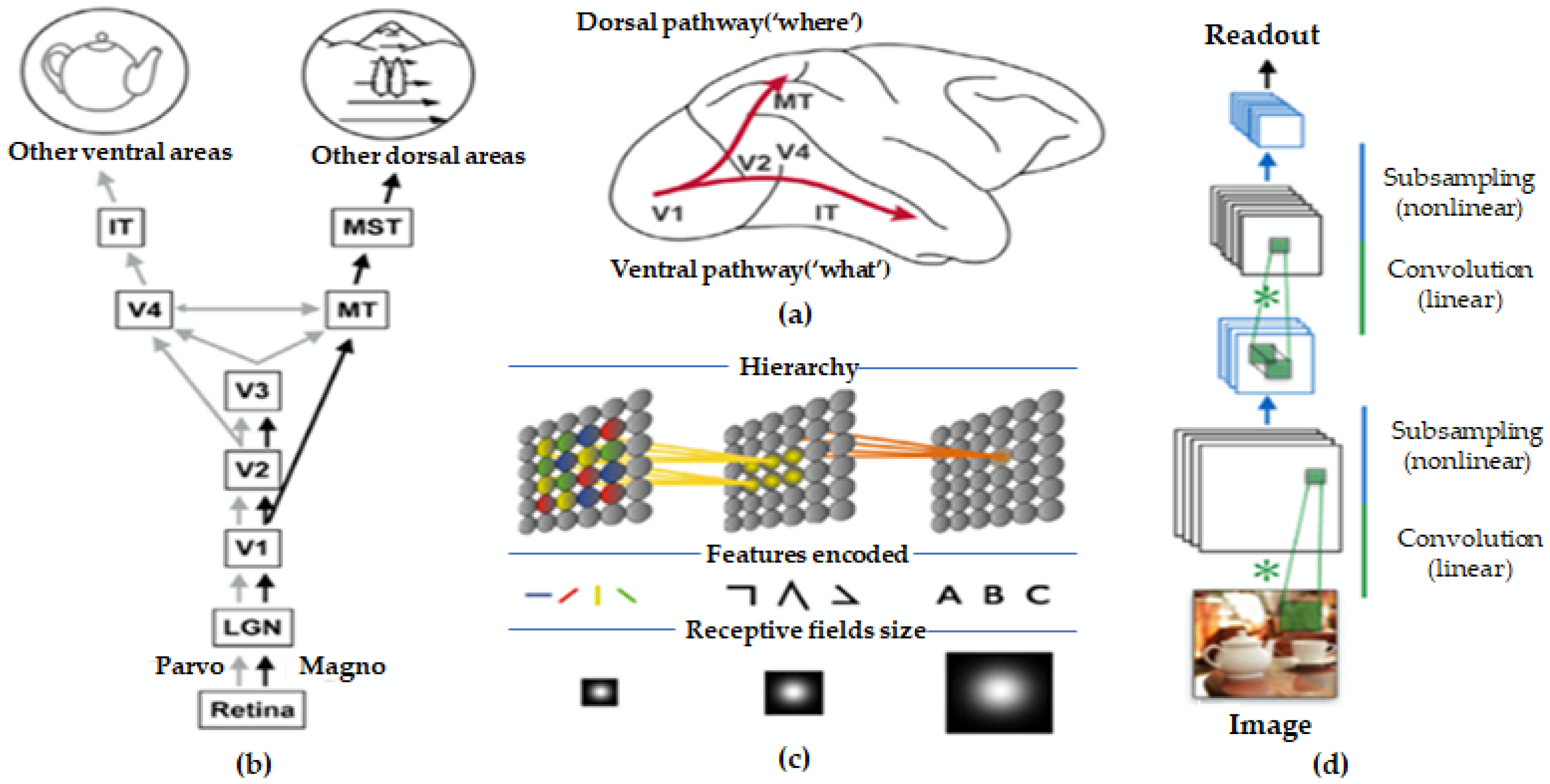
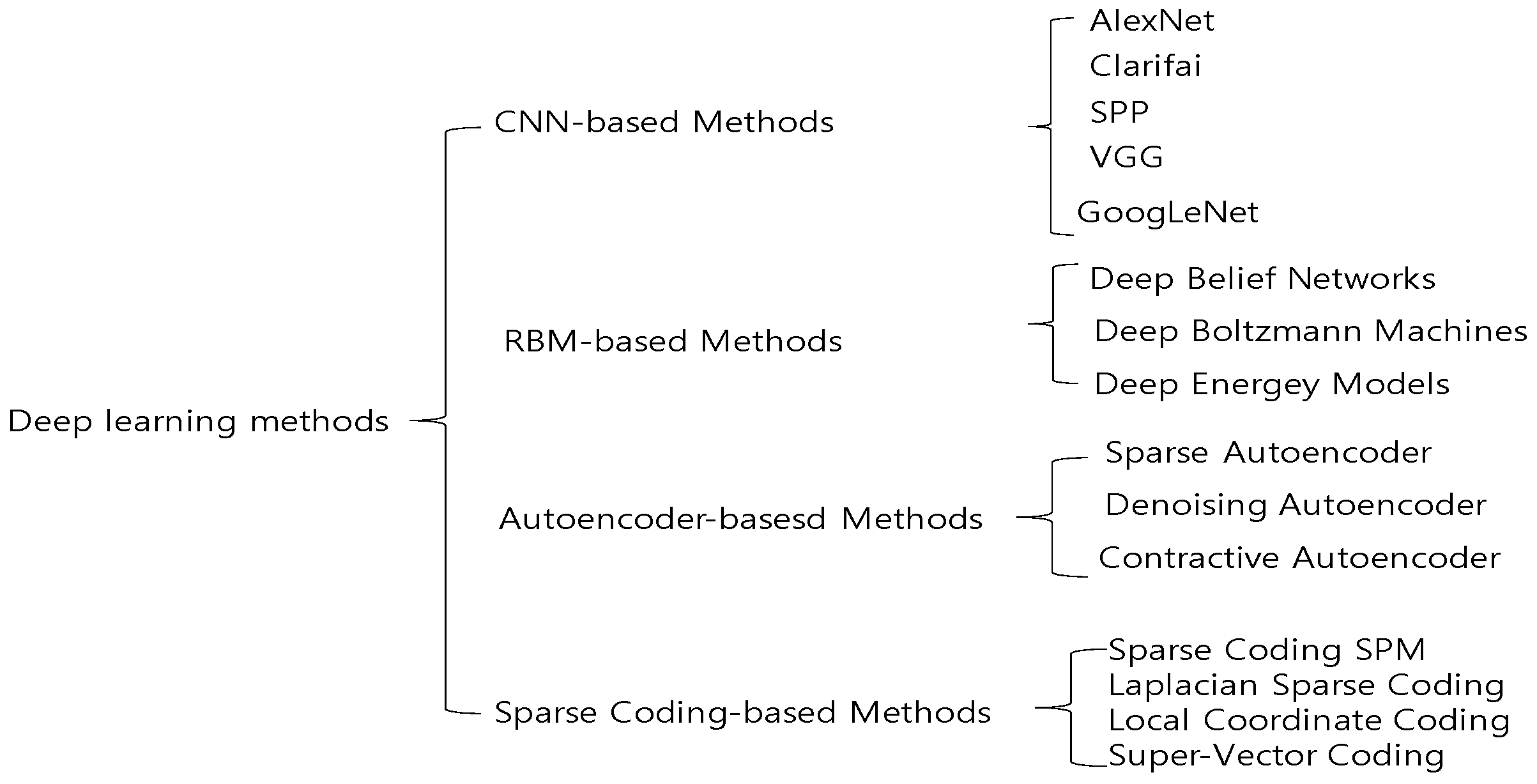
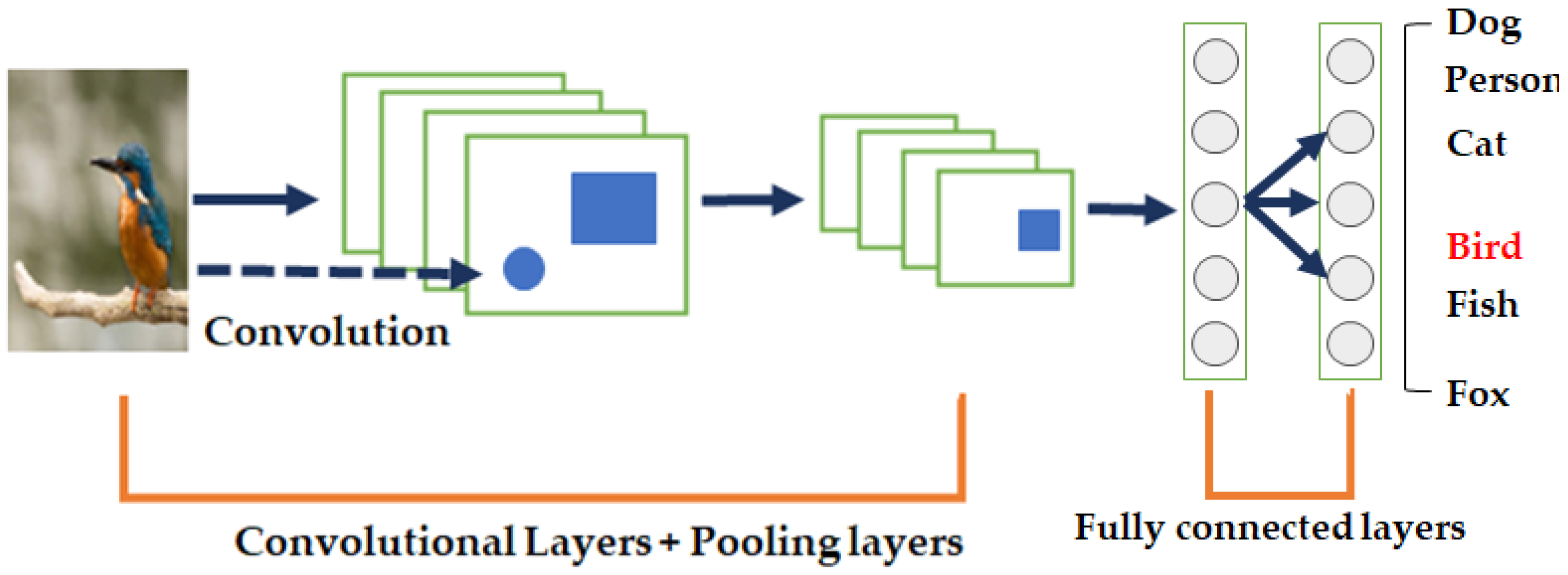
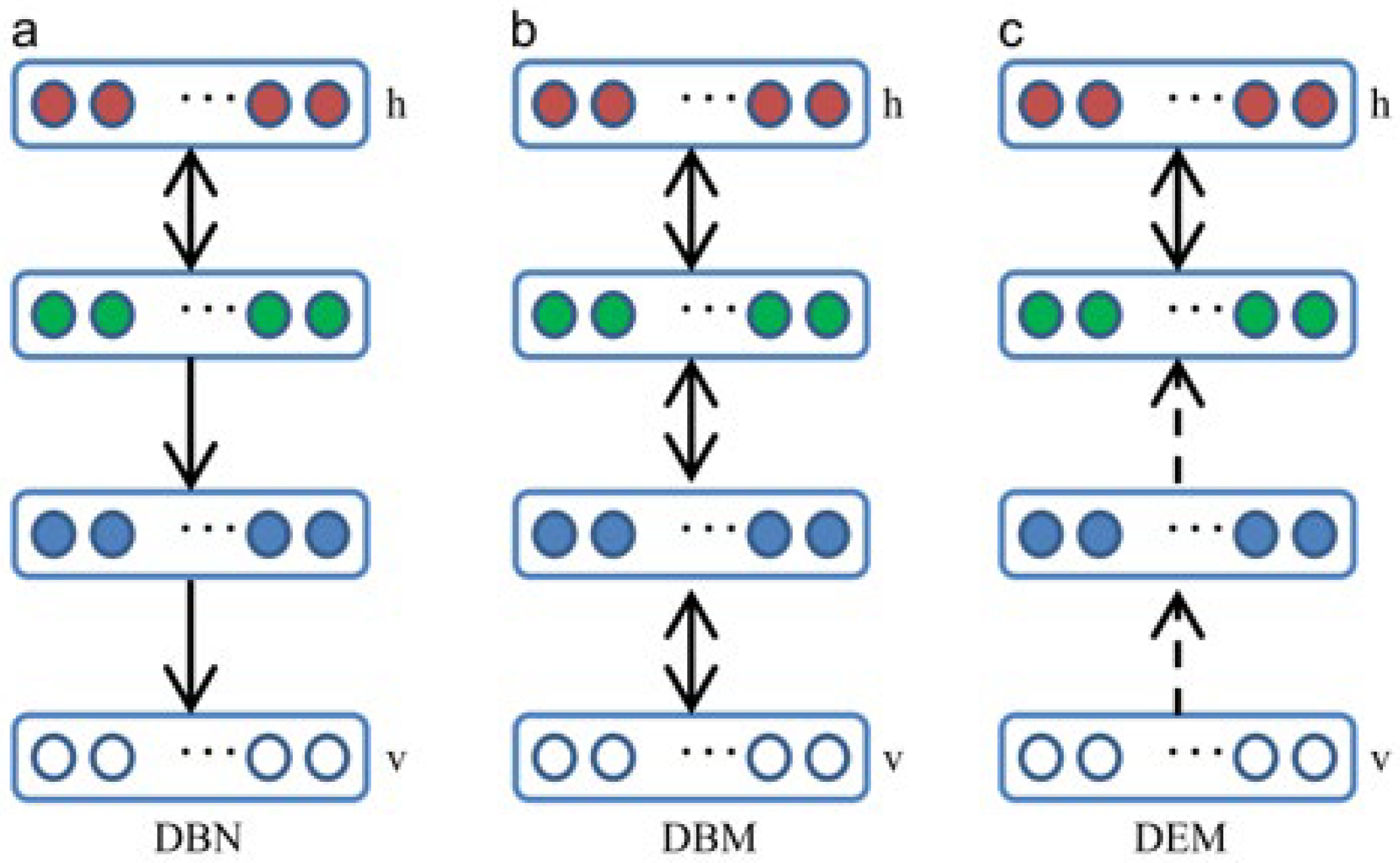
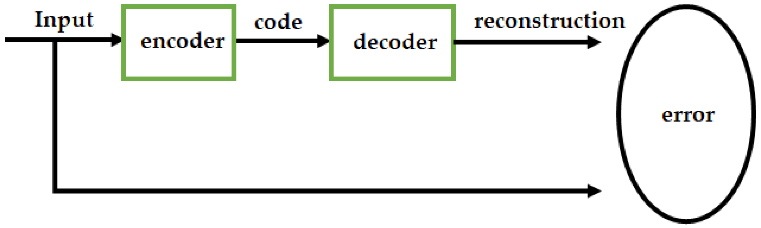
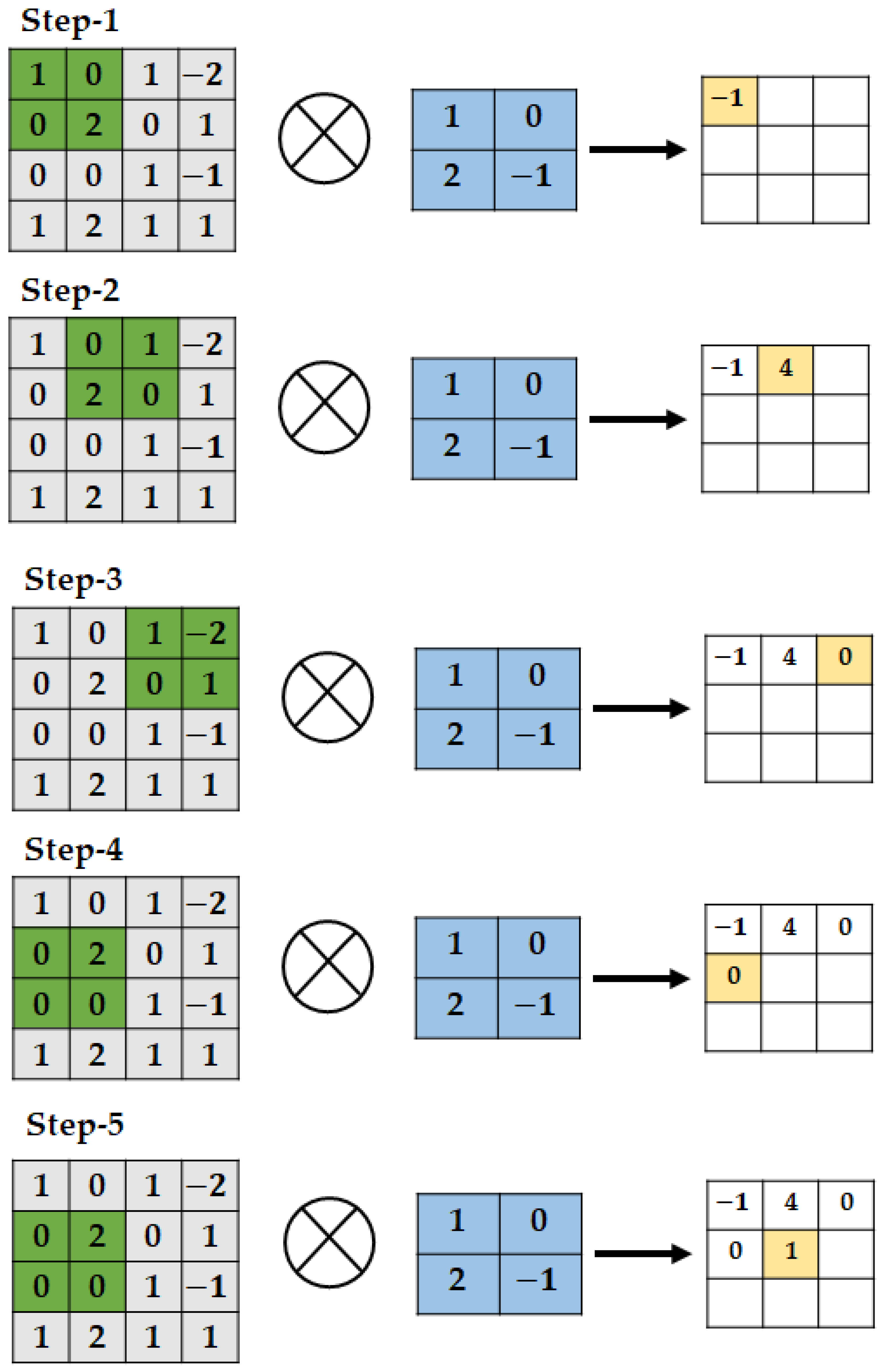
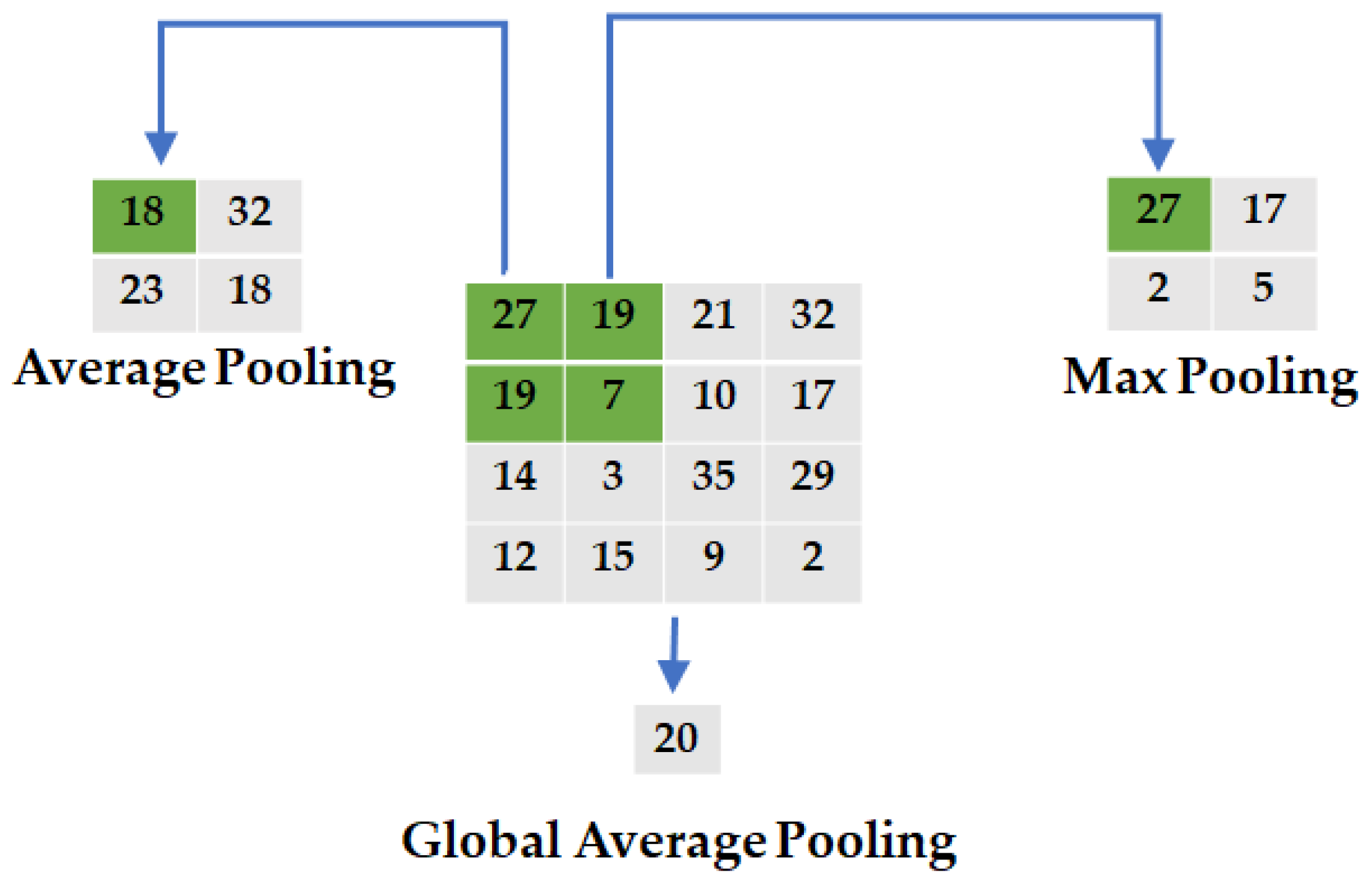
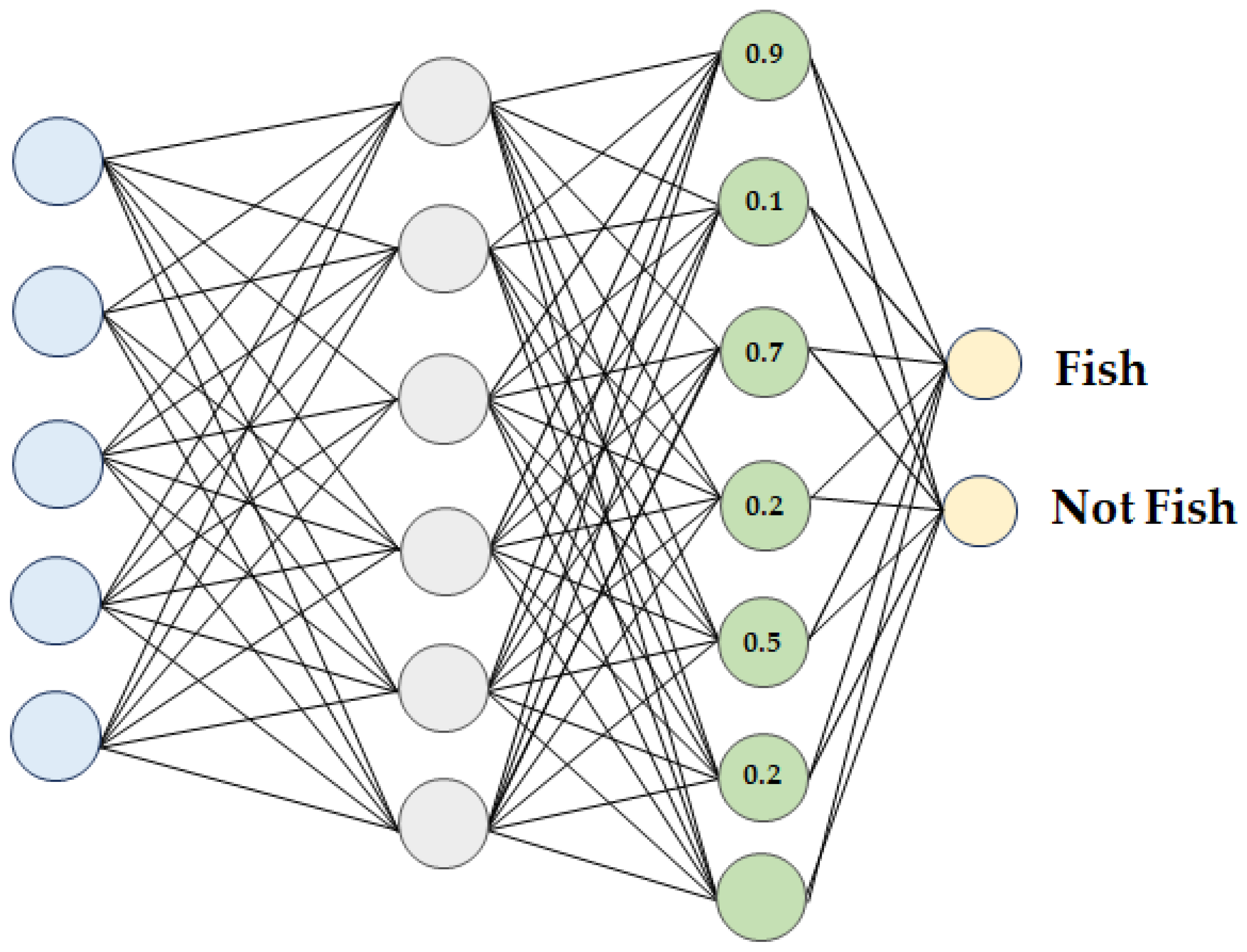
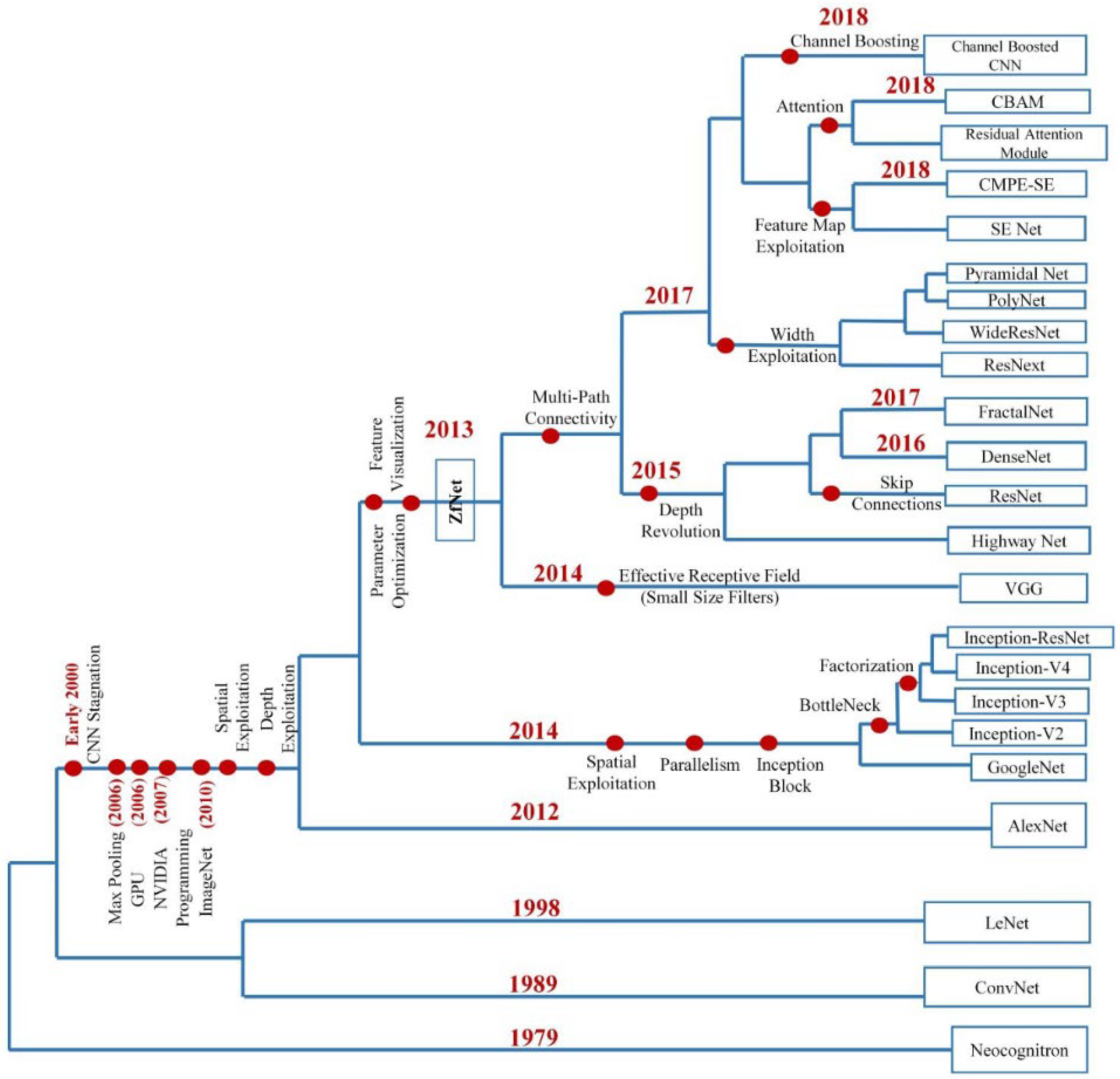
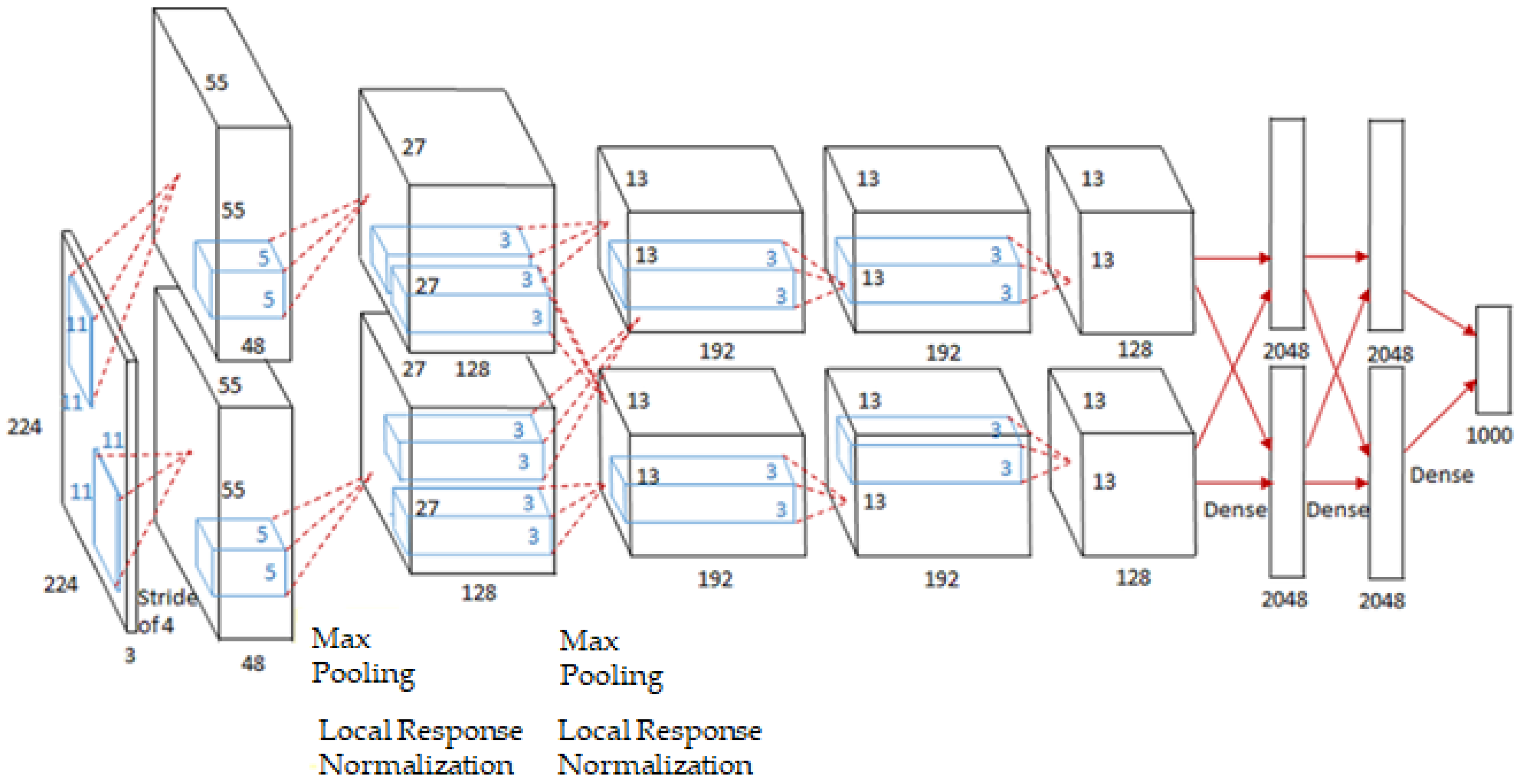
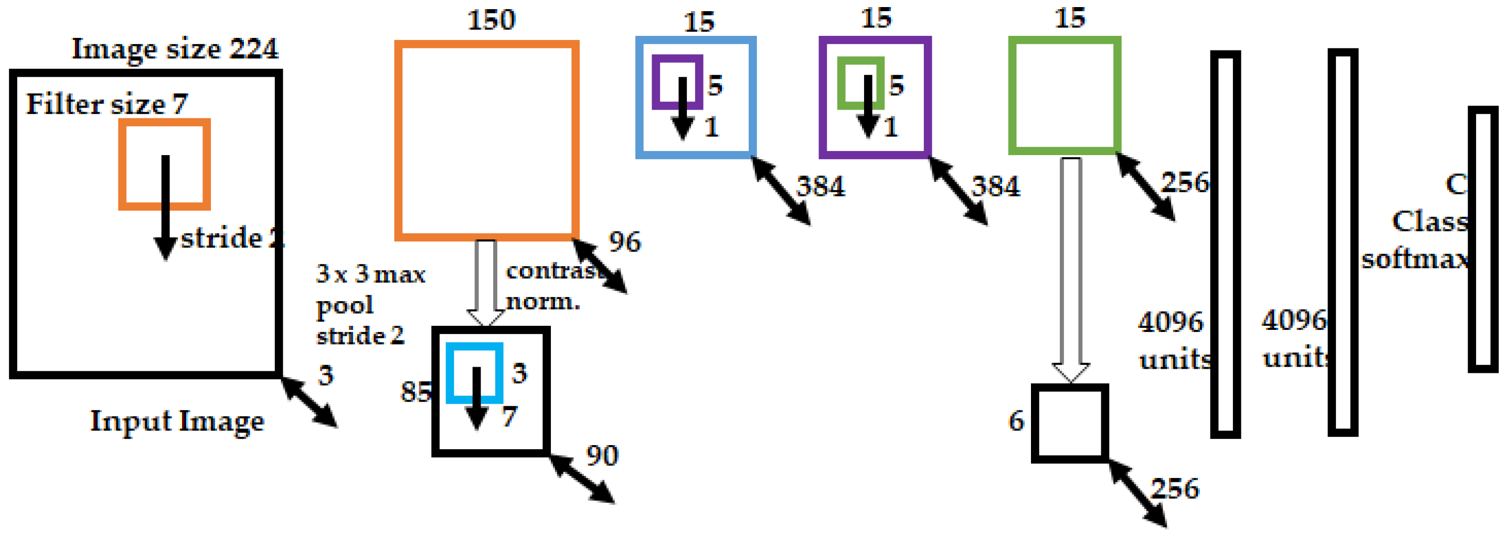
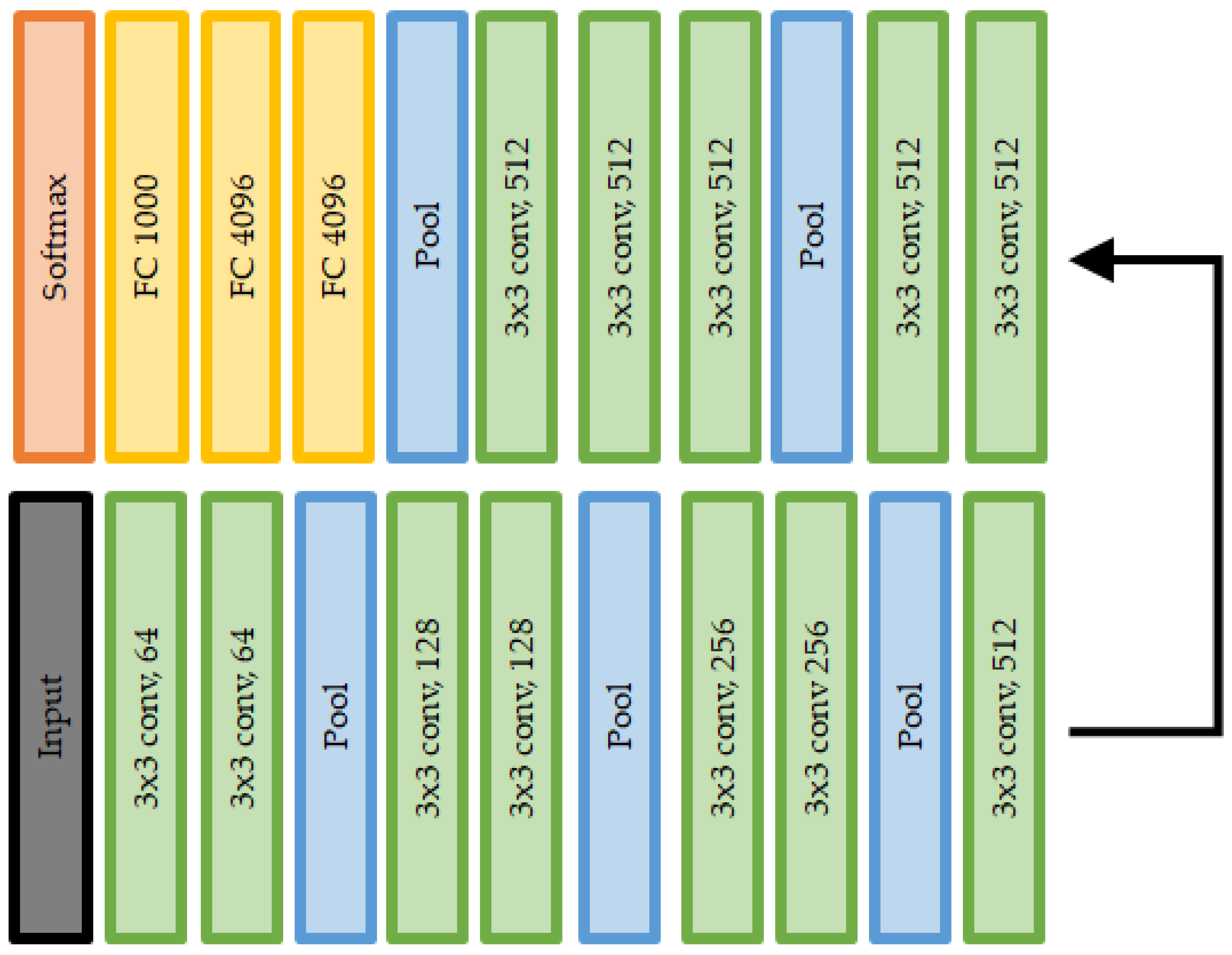
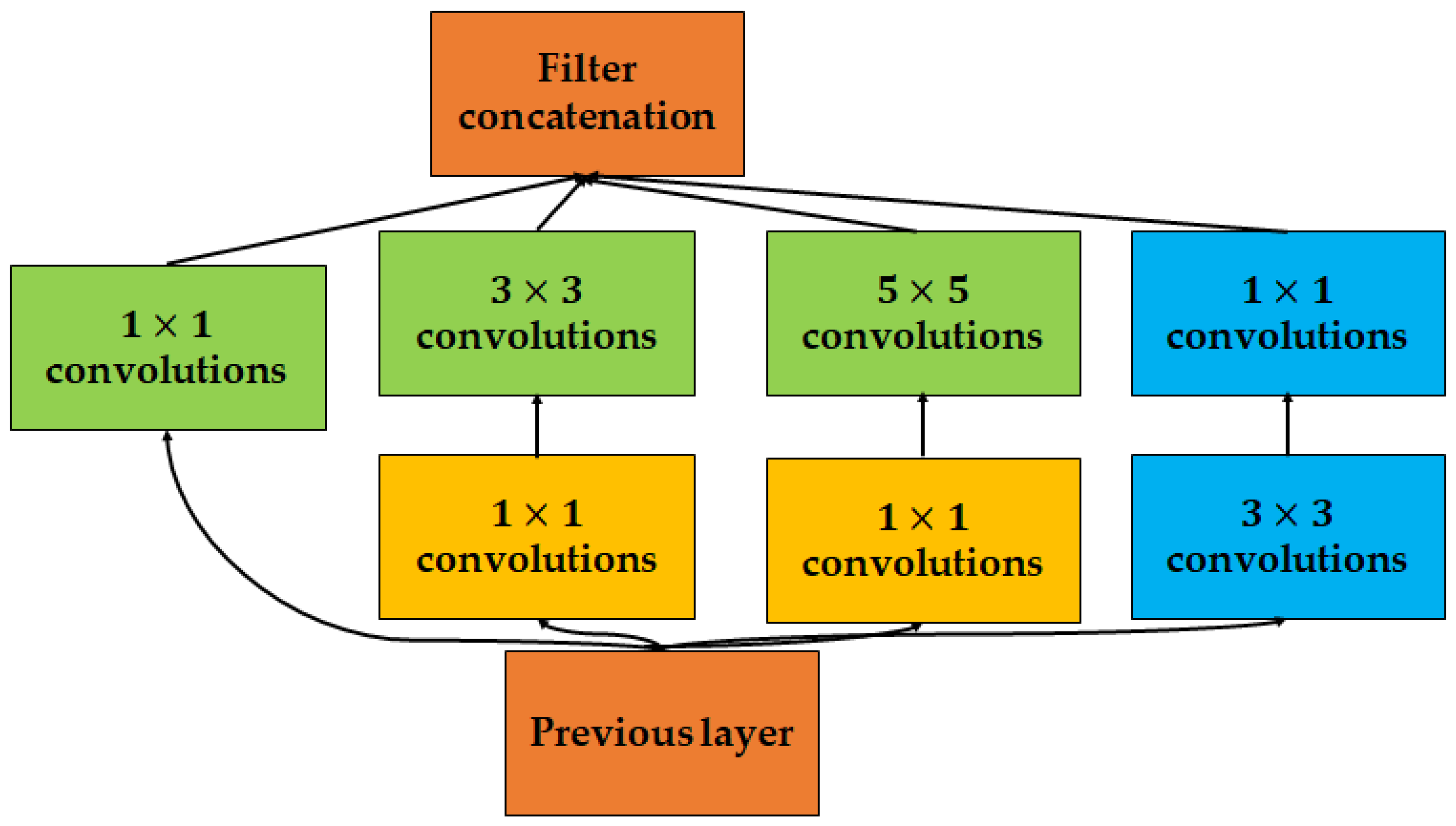
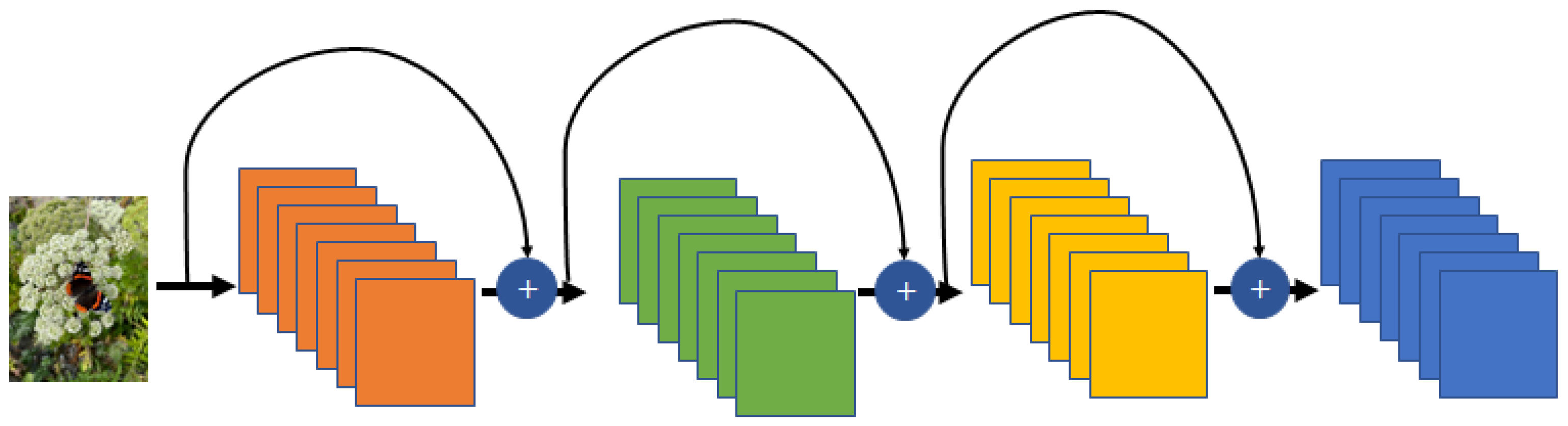
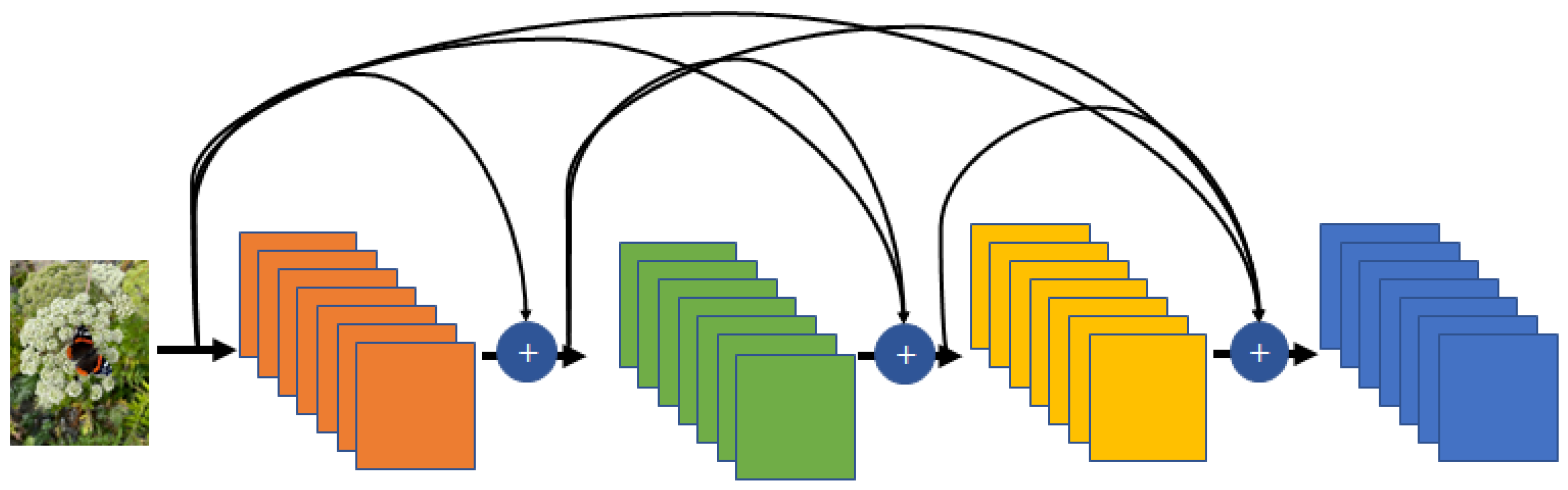
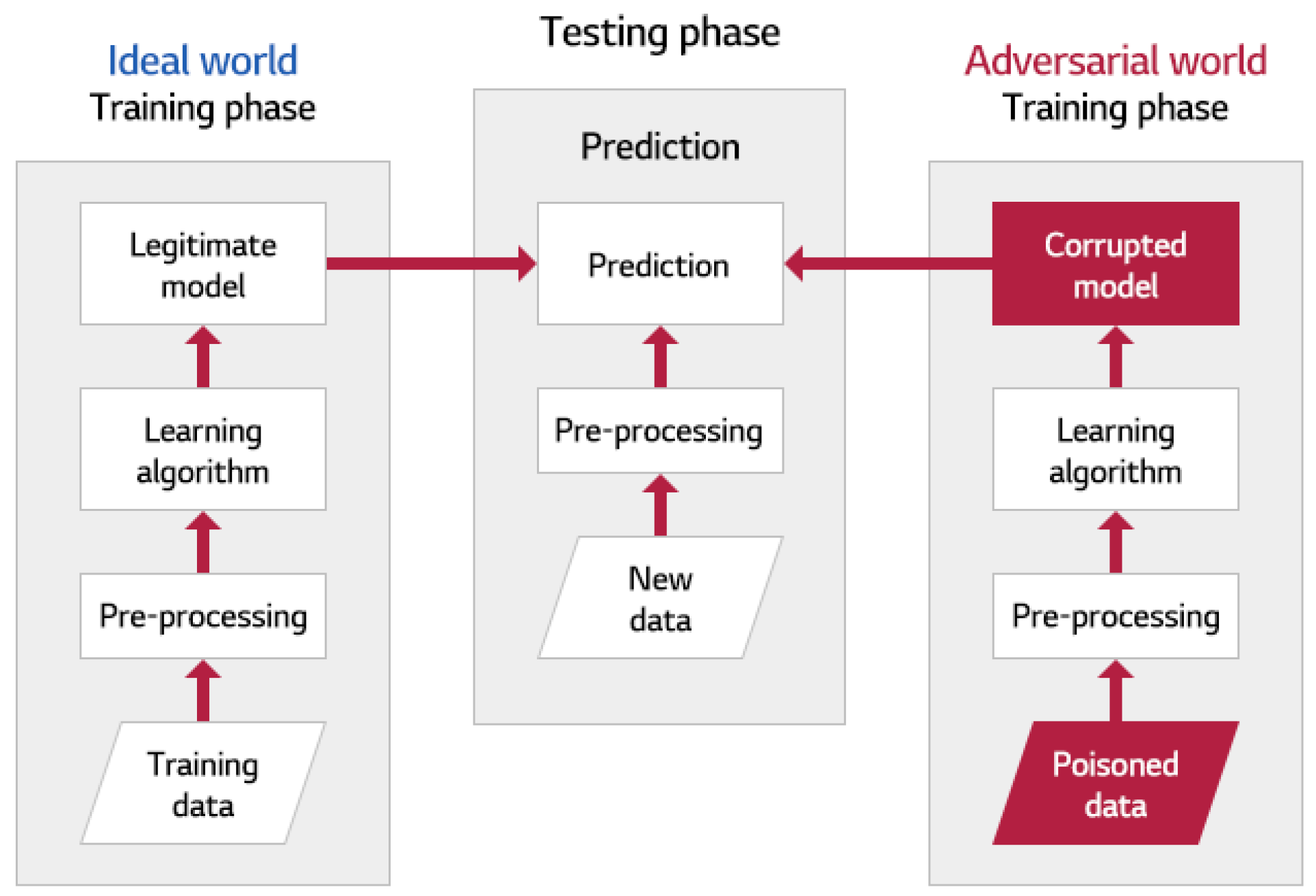
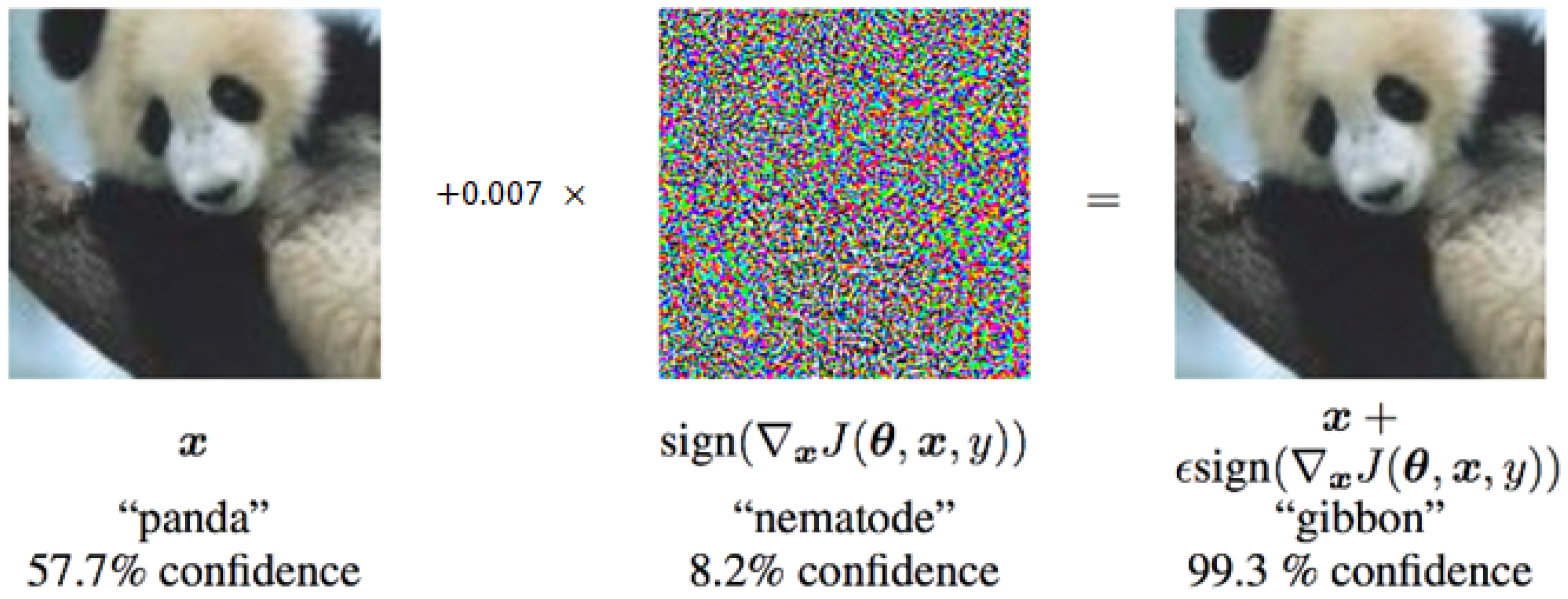
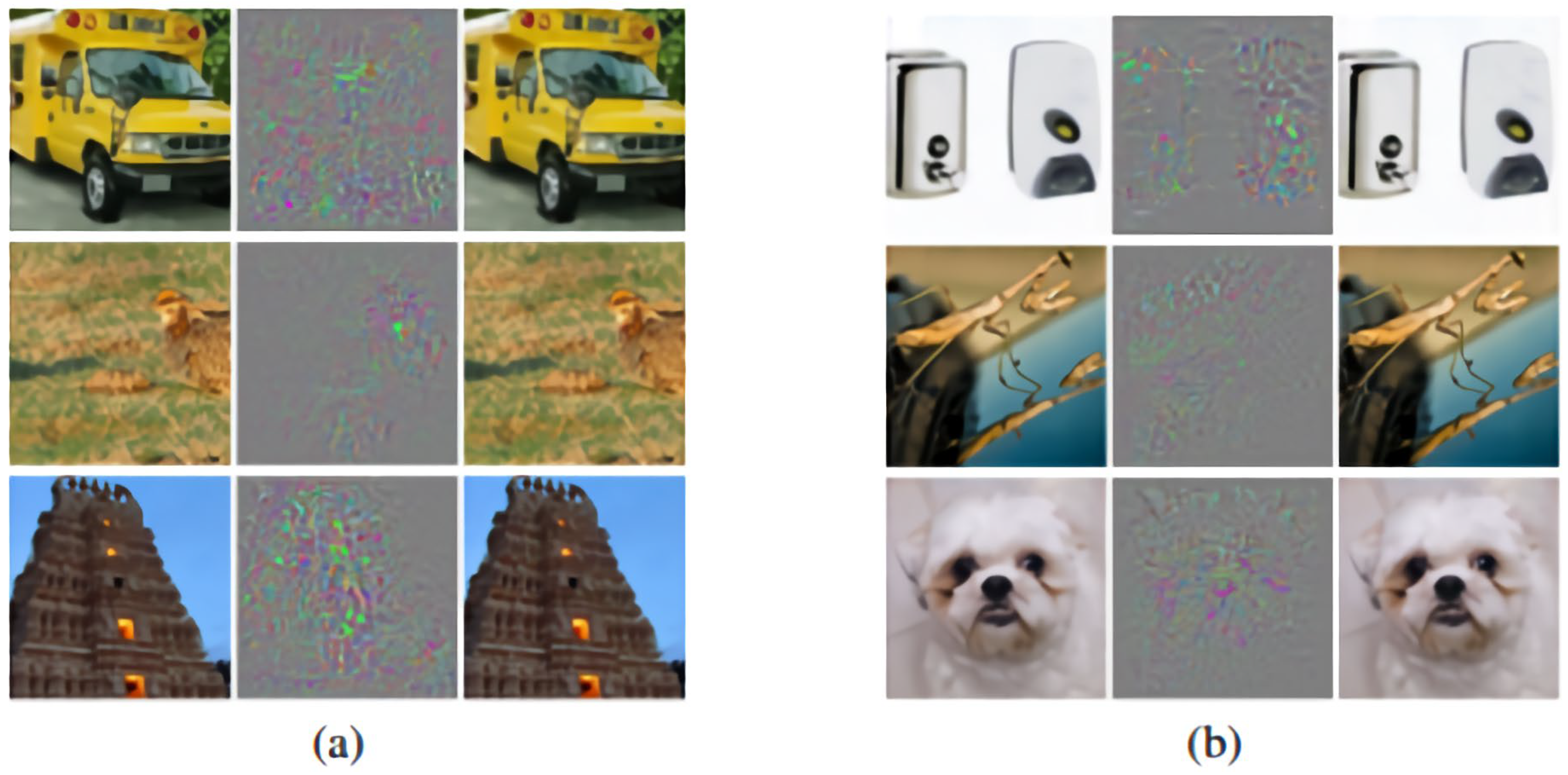
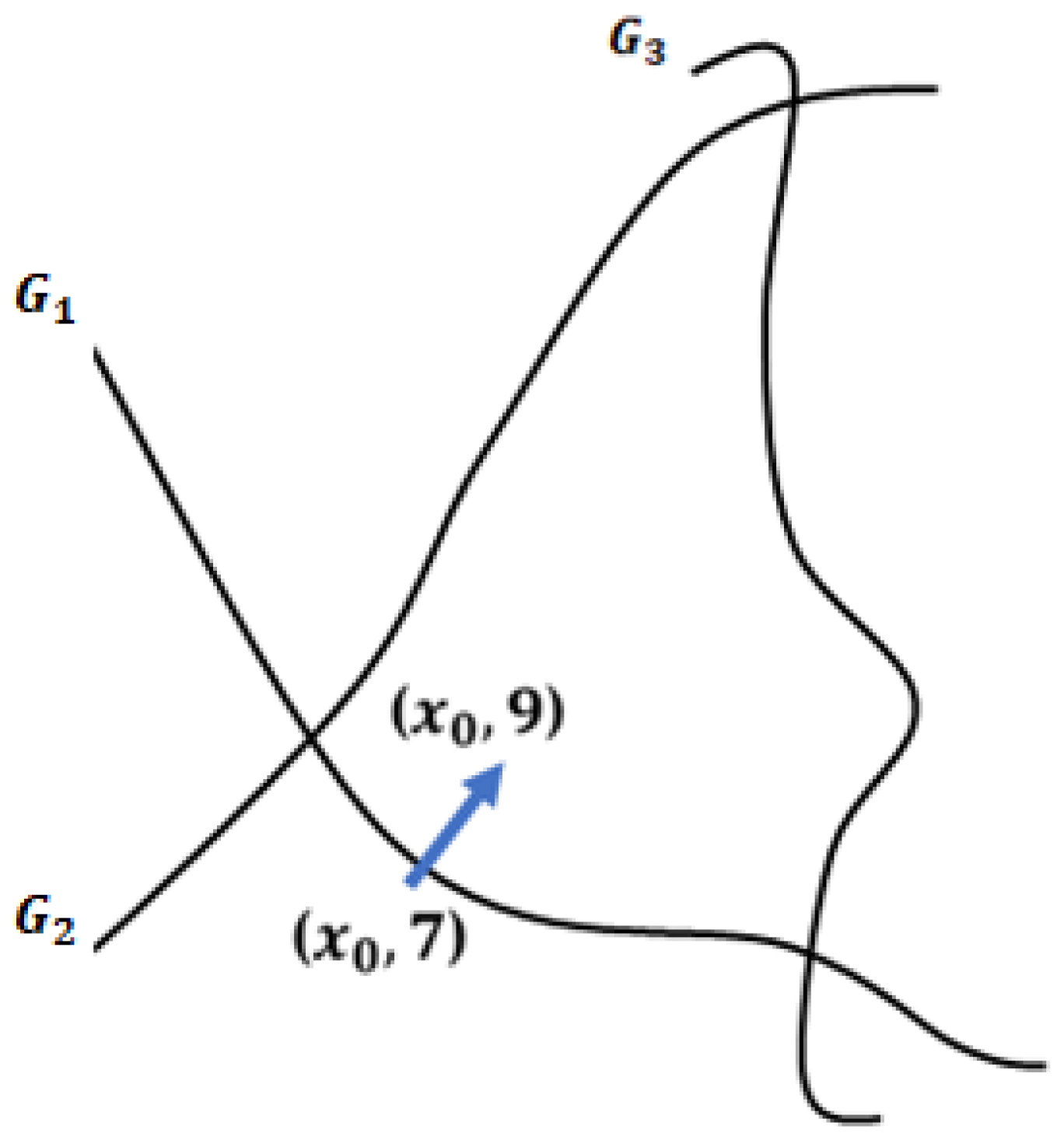
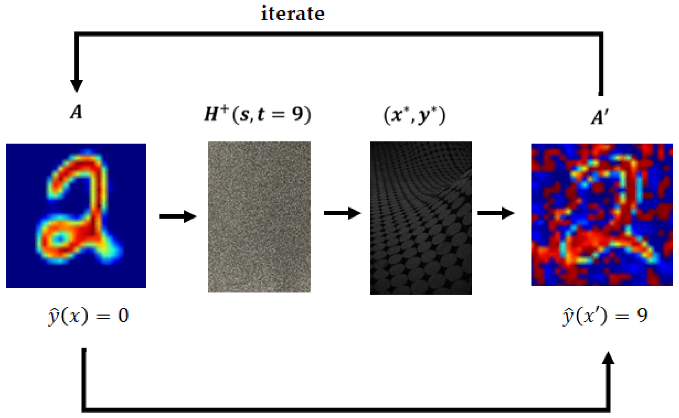
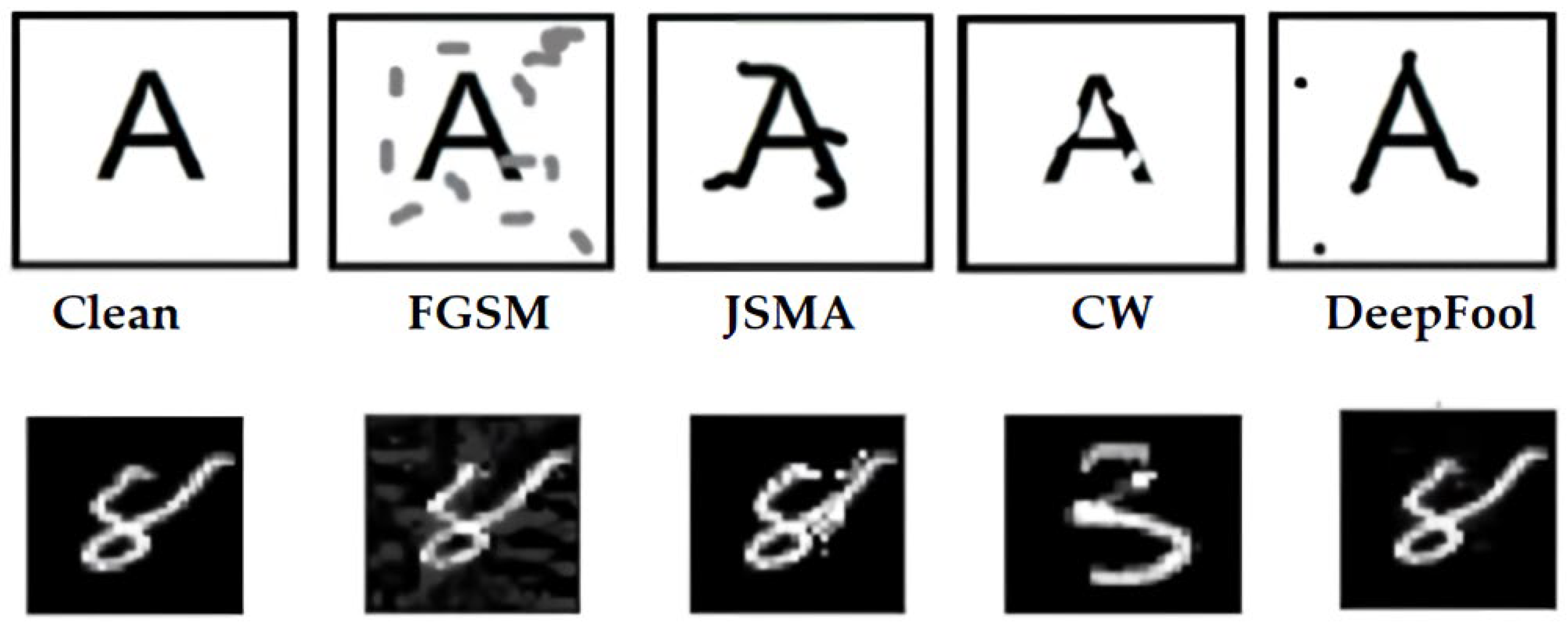
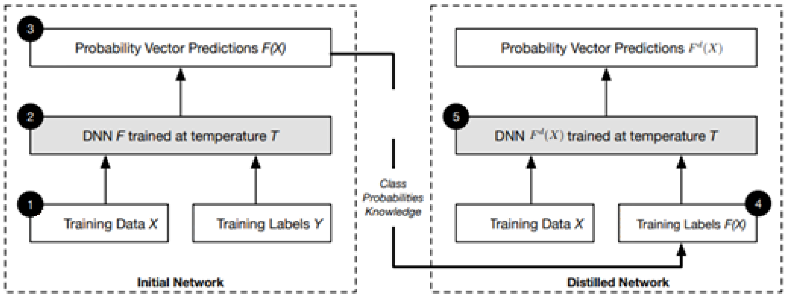
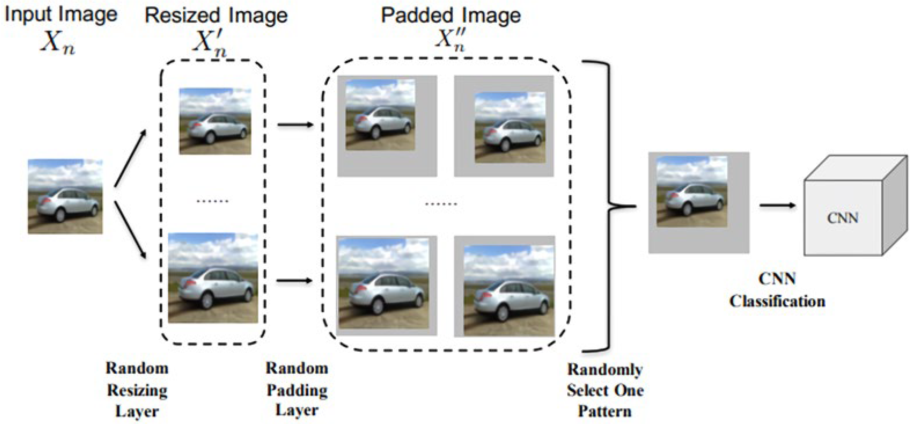
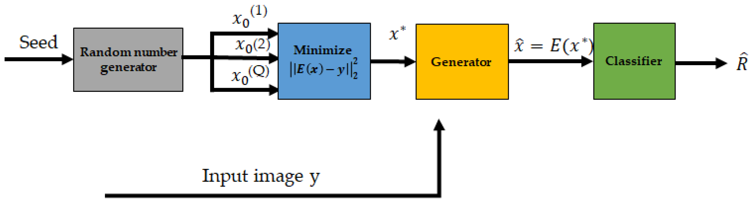
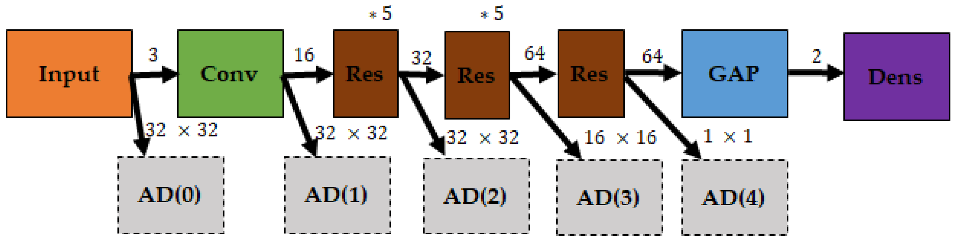
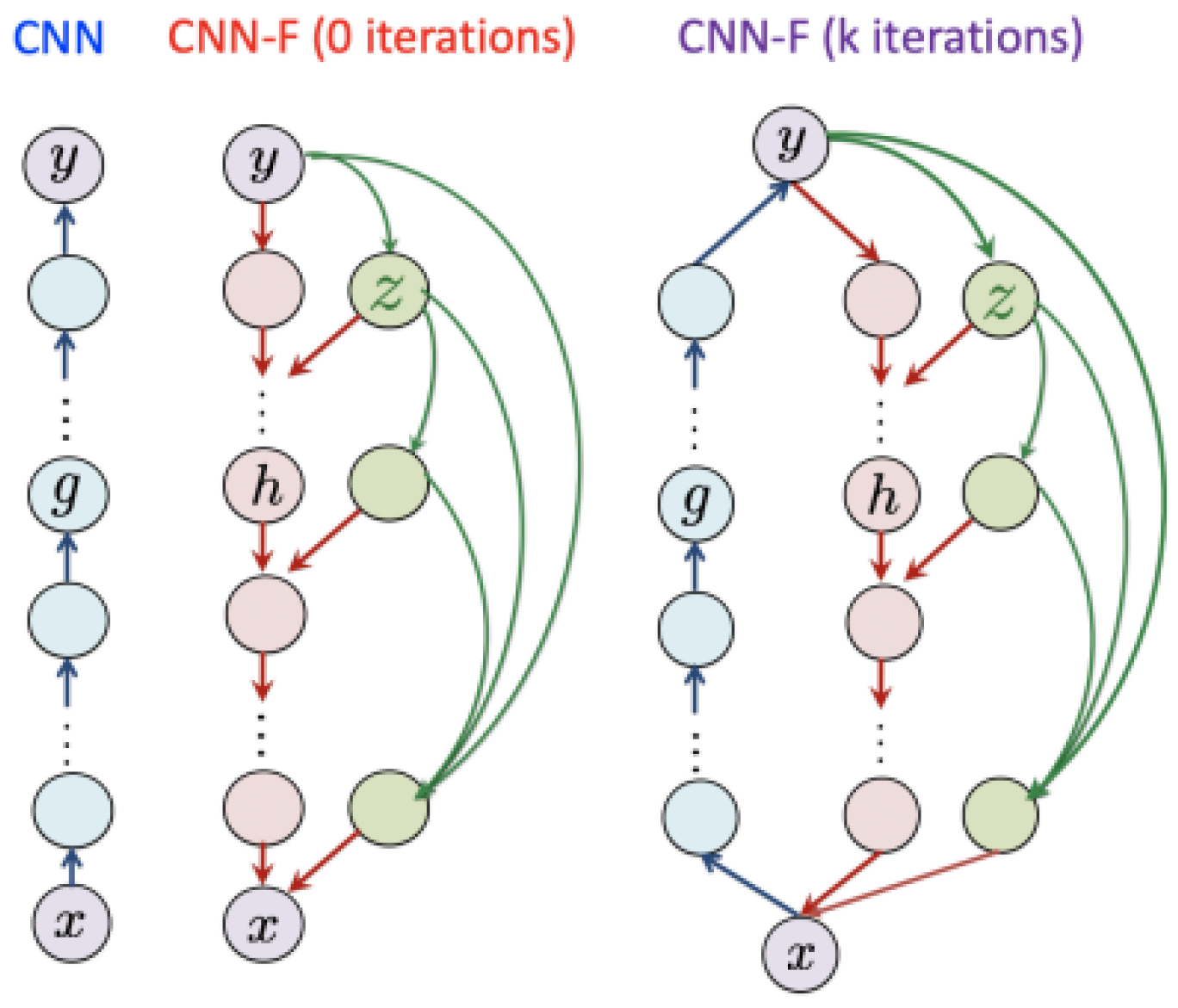
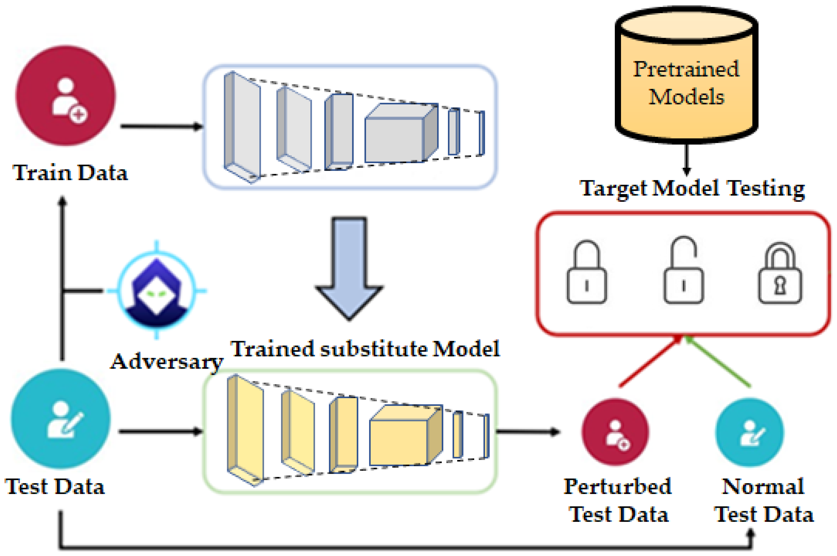
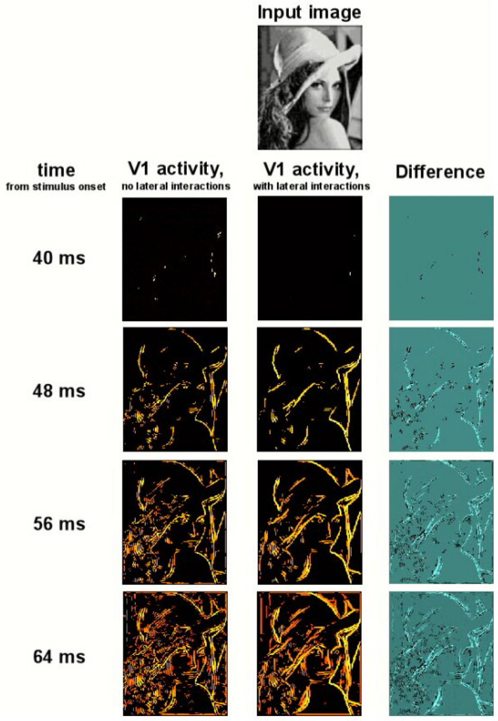
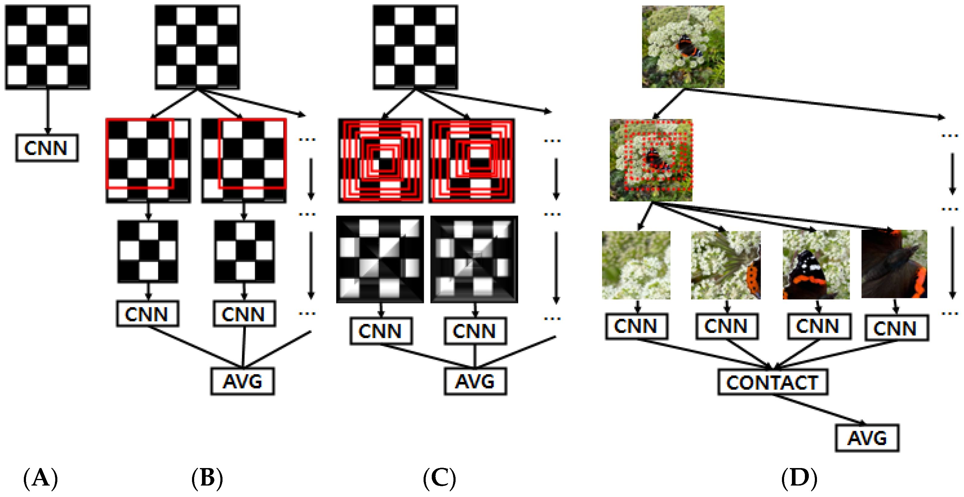
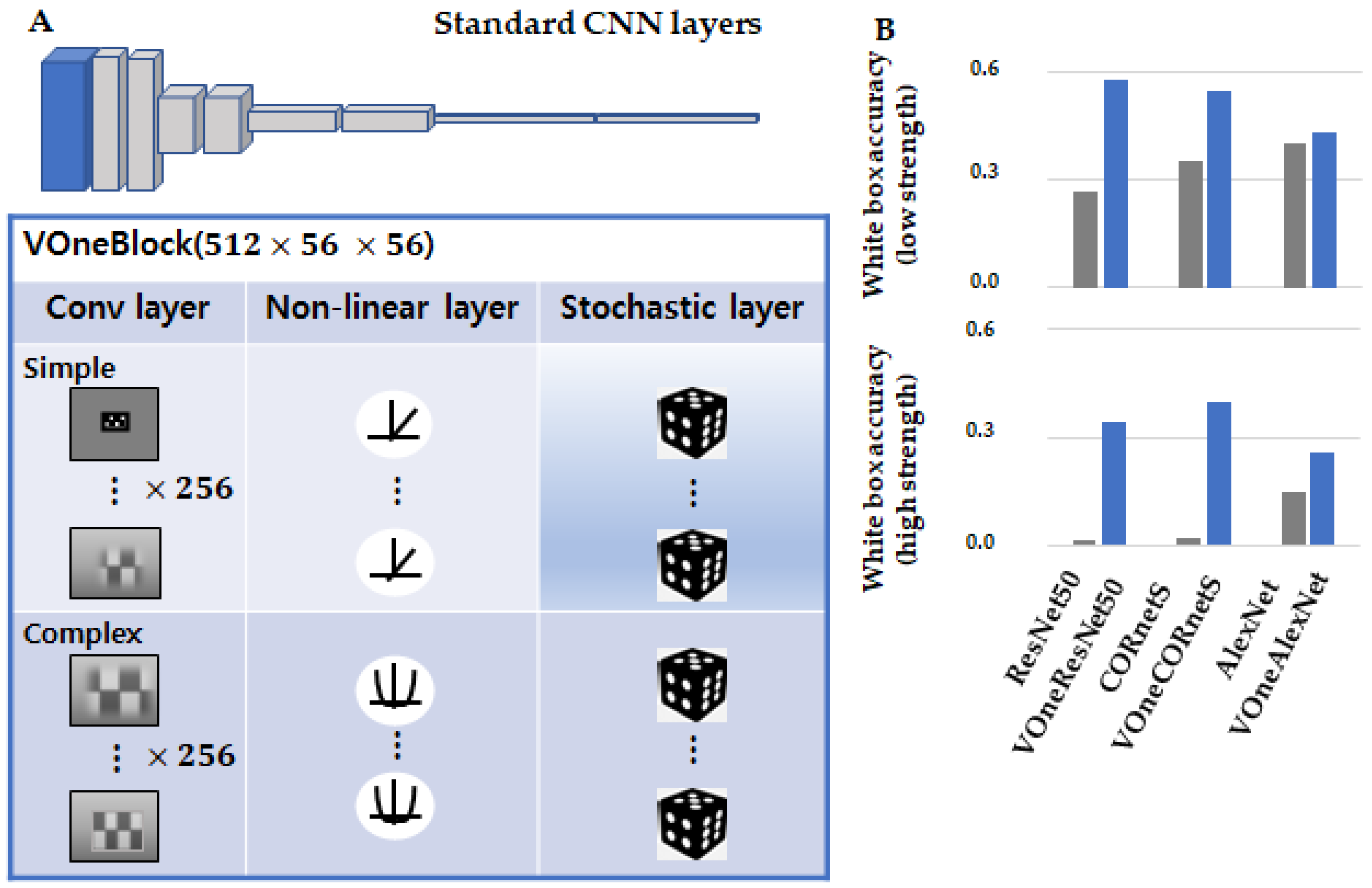
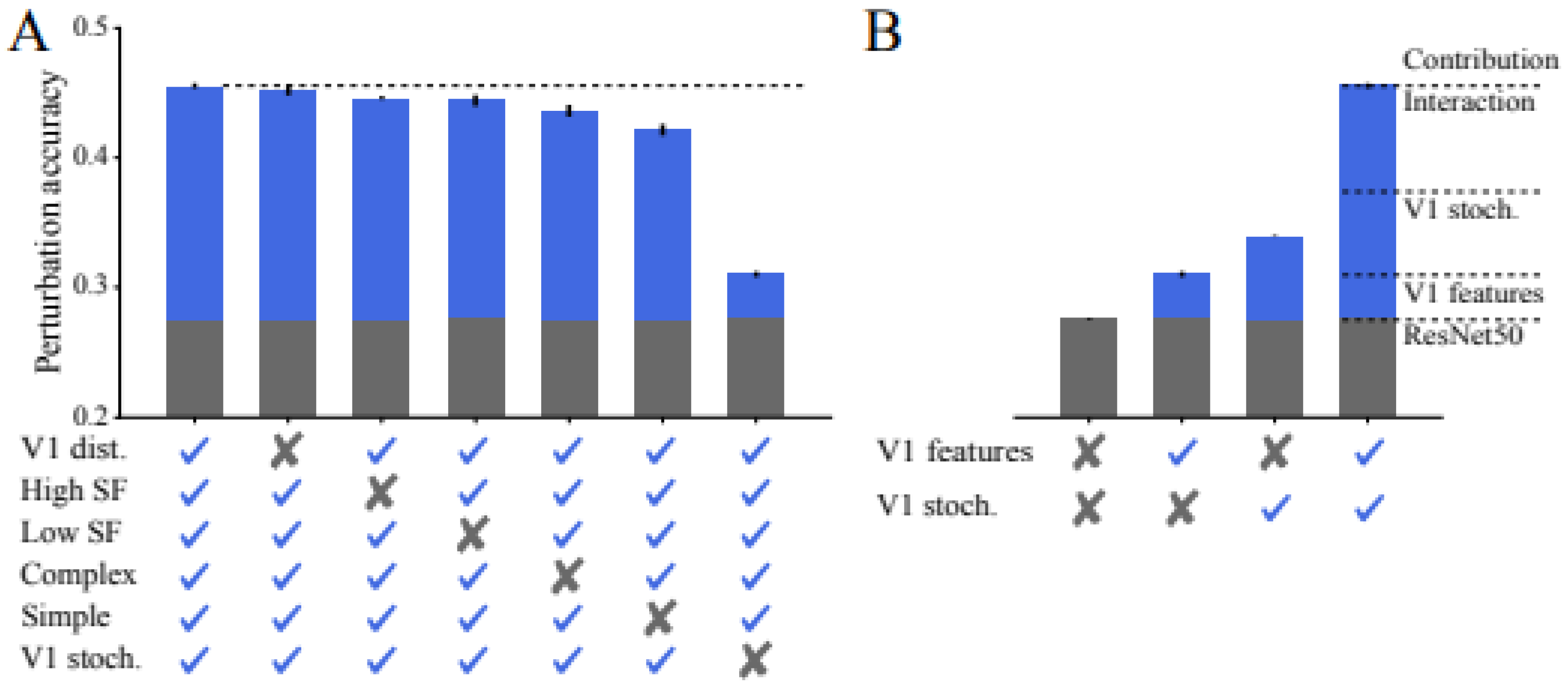
Table 1.
Adversarial attack results by integrated contour model in [151].
Table 1.
Adversarial attack results by integrated contour model in [151].
| Model | Top-1 Accuracy | Pixels | Attack Success |
|---|---|---|---|
| AlexNet | 36.1 ± 0.4 | 1 | 8.5 ± 0.4% |
| 3 | 10.6 ± 2.2% | ||
| 5 | 10.4 ± 2.1% | ||
| AlexNet + Contour | 38.0 ± 1.1 | 1 | 8.22 ± 1.8% |
| 3 | 9.76 ± 20% | ||
| 5 | 9.55 ± 1.75% |
Table 2.
The results of adversarial tests for two hidden layers artificial neural network trained by the GLR with different activation and loss functions in [161].
Table 2.
The results of adversarial tests for two hidden layers artificial neural network trained by the GLR with different activation and loss functions in [161].
| Activations + Entropy | Orig. | Adv_L_BFGS | Adv_FGSM |
|---|---|---|---|
| Sigmoid (trained by BP) | 0.96 | 0.57 | 0.28 |
| Sigmoid | 0.94 | 0.77 | 0.45 |
| Threshold | 0.93 | 0.73 | 0.52 |
| 0.94 | 0.78 | 0.53 | |
| Activations + 0–1 loss | Orig. | Adv_L_BFGS | Adv_FGSM |
| Sigmoid | 0.84 | 0.76 | 0.58 |
| Threshold | 0.83 | 0.72 | 0.57 |
Disclaimer/Publisher’s Note: The statements, opinions and data contained in all publications are solely those of the individual author(s) and contributor(s) and not of MDPI and/or the editor(s). MDPI and/or the editor(s) disclaim responsibility for any injury to people or property resulting from any ideas, methods, instructions or products referred to in the content. |
© 2023 by the authors. Licensee MDPI, Basel, Switzerland. This article is an open access article distributed under the terms and conditions of the Creative Commons Attribution (CC BY) license (https://creativecommons.org/licenses/by/4.0/).
Share and Cite
MDPI and ACS Style
Lee, Y.; Kim, J. Robustness of Deep Learning Models for Vision Tasks. Appl. Sci. 2023, 13, 4422. https://doi.org/10.3390/app13074422
AMA Style
Lee Y, Kim J. Robustness of Deep Learning Models for Vision Tasks. Applied Sciences. 2023; 13(7):4422. https://doi.org/10.3390/app13074422
Chicago/Turabian StyleLee, Youngseok, and Jongweon Kim. 2023. "Robustness of Deep Learning Models for Vision Tasks" Applied Sciences 13, no. 7: 4422. https://doi.org/10.3390/app13074422
Note that from the first issue of 2016, this journal uses article numbers instead of page numbers. See further details here.