
Prediction Models of Saturated Vapor Pressure, Saturated Density, Surface Tension, Viscosity and Thermal Conductivity of Electronic Fluoride Liquids in Two-Phase Liquid Immersion Cooling Systems: A Comprehensive Review
Abstract
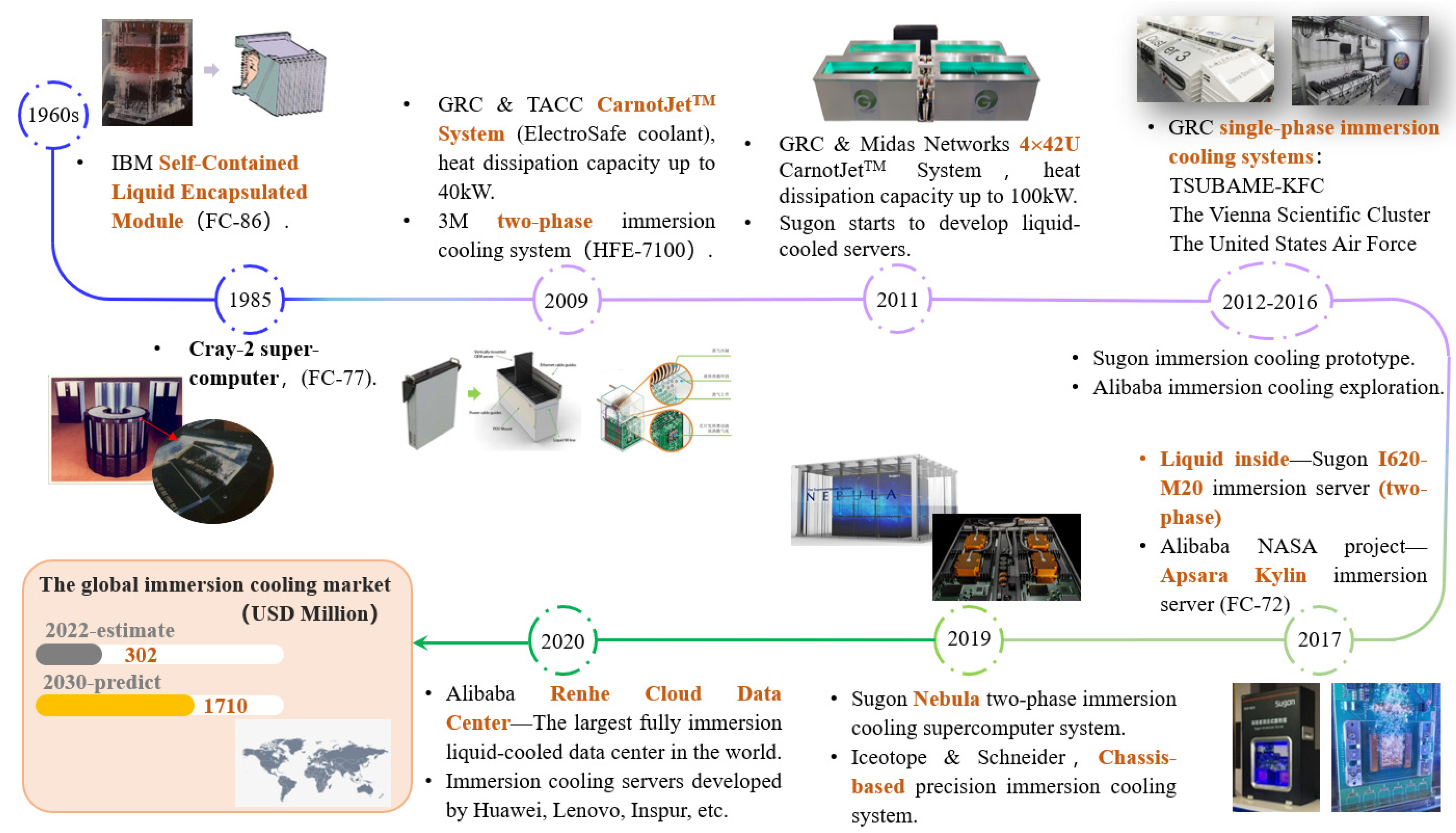
:1. Introduction
2. Basic Analysis of Prediction Models and Model Verification
2.1. Analysis of Key Thermophysical Properties
2.2. Screening of Coolants for Model Verification
3. Prediction of Thermophysical Properties of Electronic Fluoride Liquids for Two-Phase Liquid Immersion Cooling Systems
3.1. Parameters Required for the Prediction of Thermophysical Properties
3.2. Prediction Models of Saturated Vapor Pressure and Saturated Density
3.2.1. Prediction Models of Saturated Vapor Pressure and Saturated Density
Peng–Robinson Equation of State and Its Modified Models
- ➀
- Modification of α function
- ➁
- Specific volume translation modification method
- ➂
- Modification of parameters a and b
Patel–Teja Equation of State
NEOS Model
3.2.2. Criterion of Iterative Computations for Comparison of Different Prediction Models
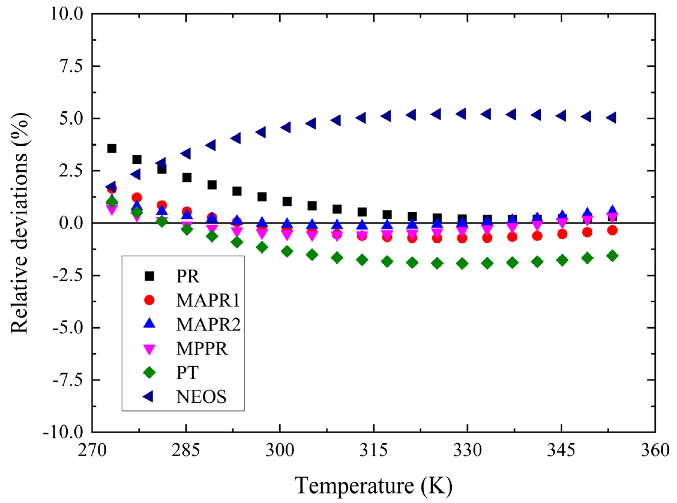
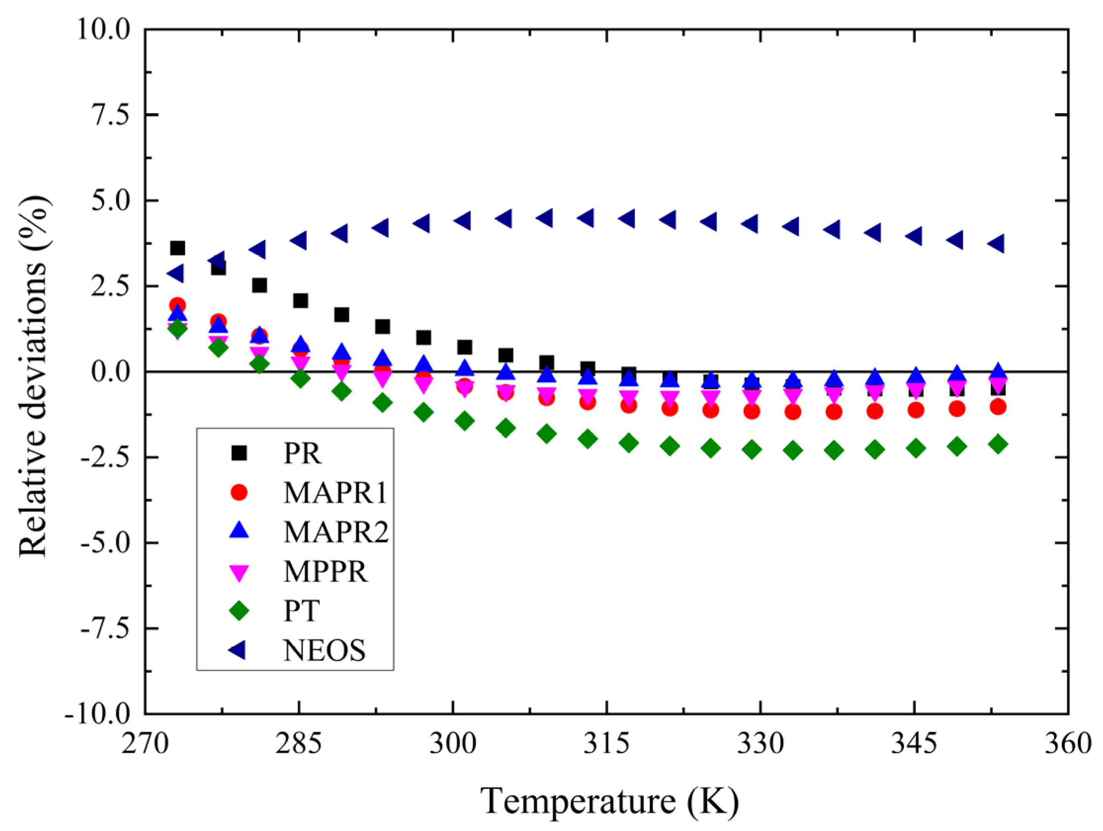
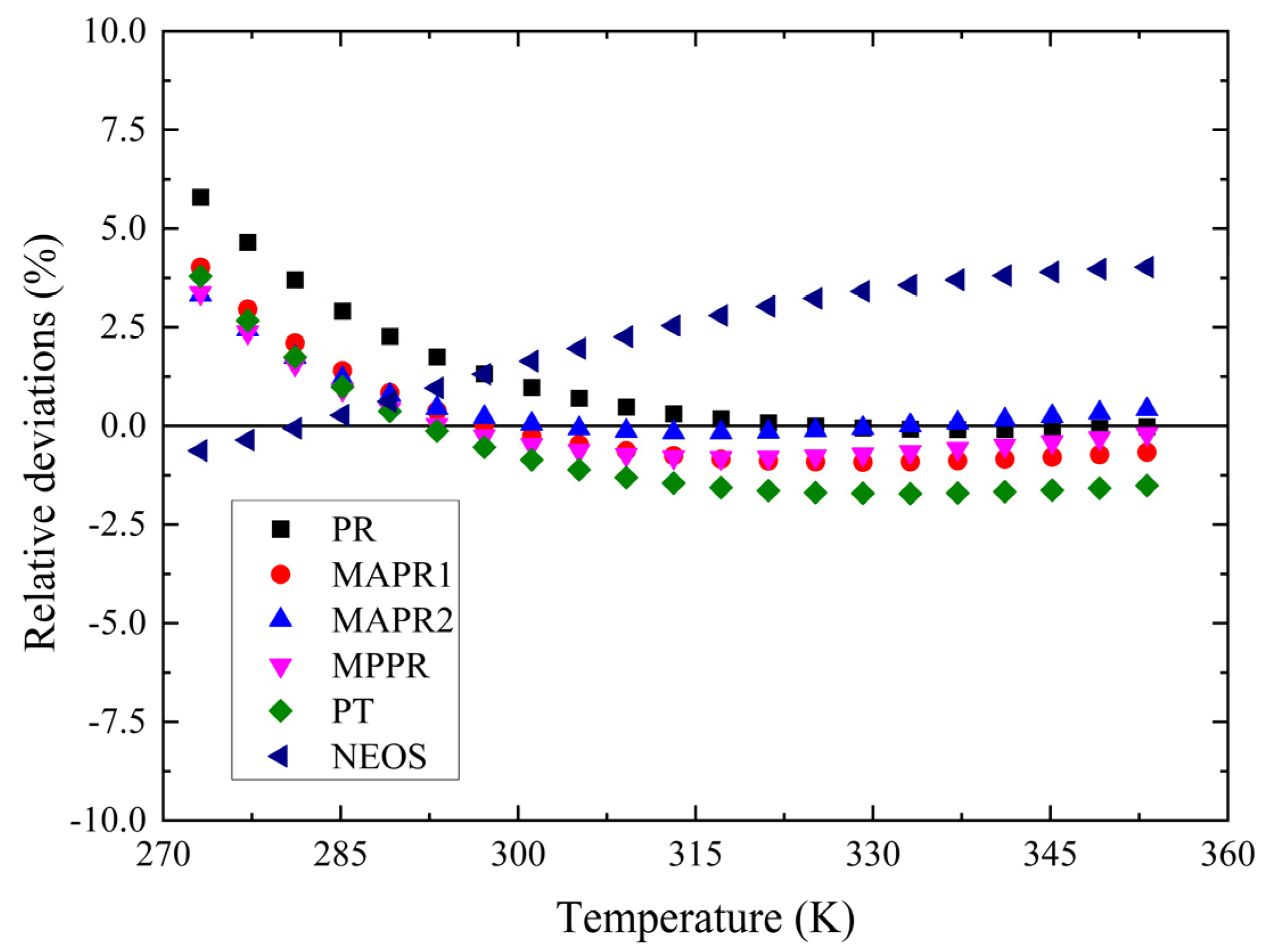
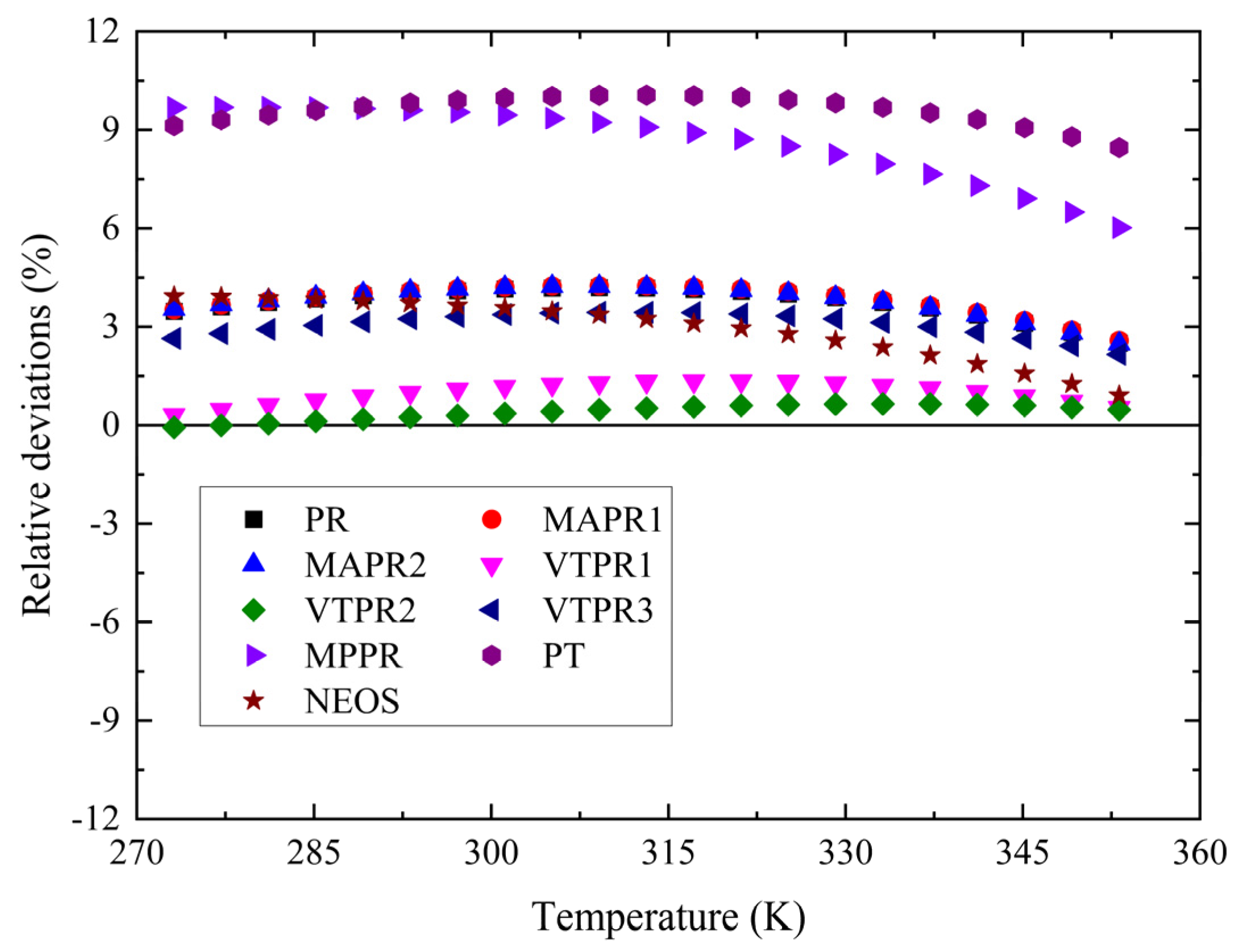
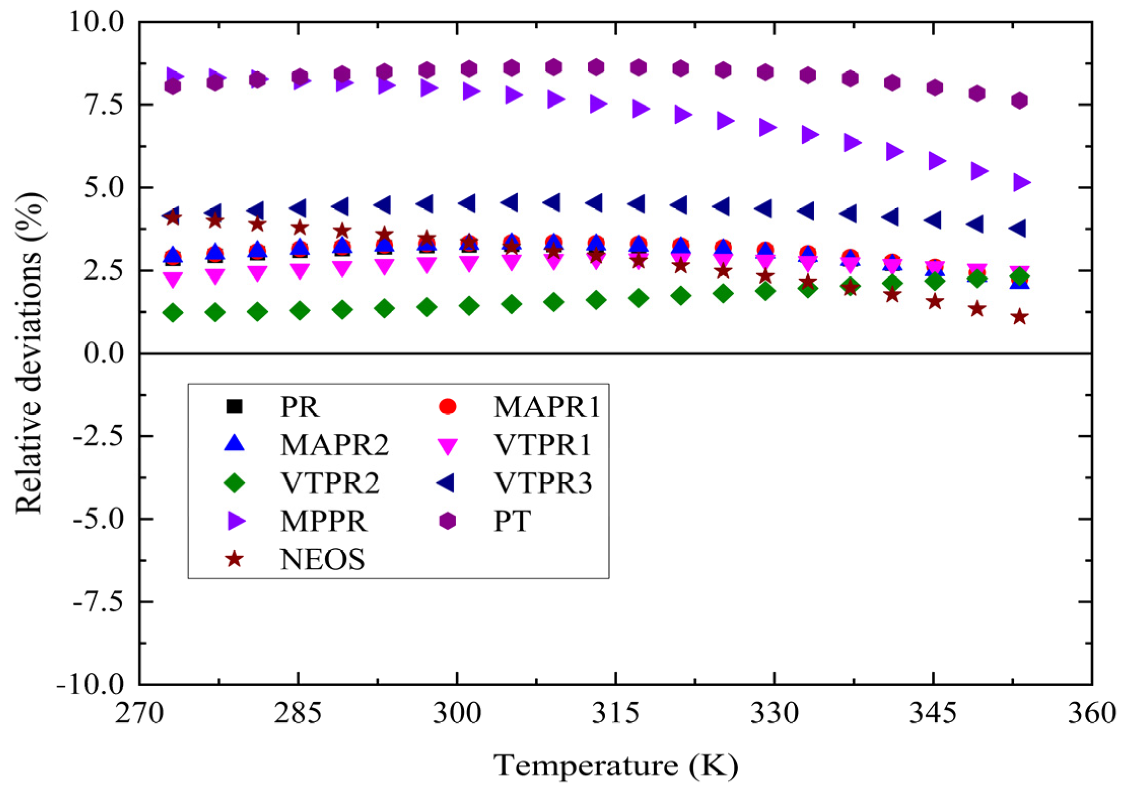
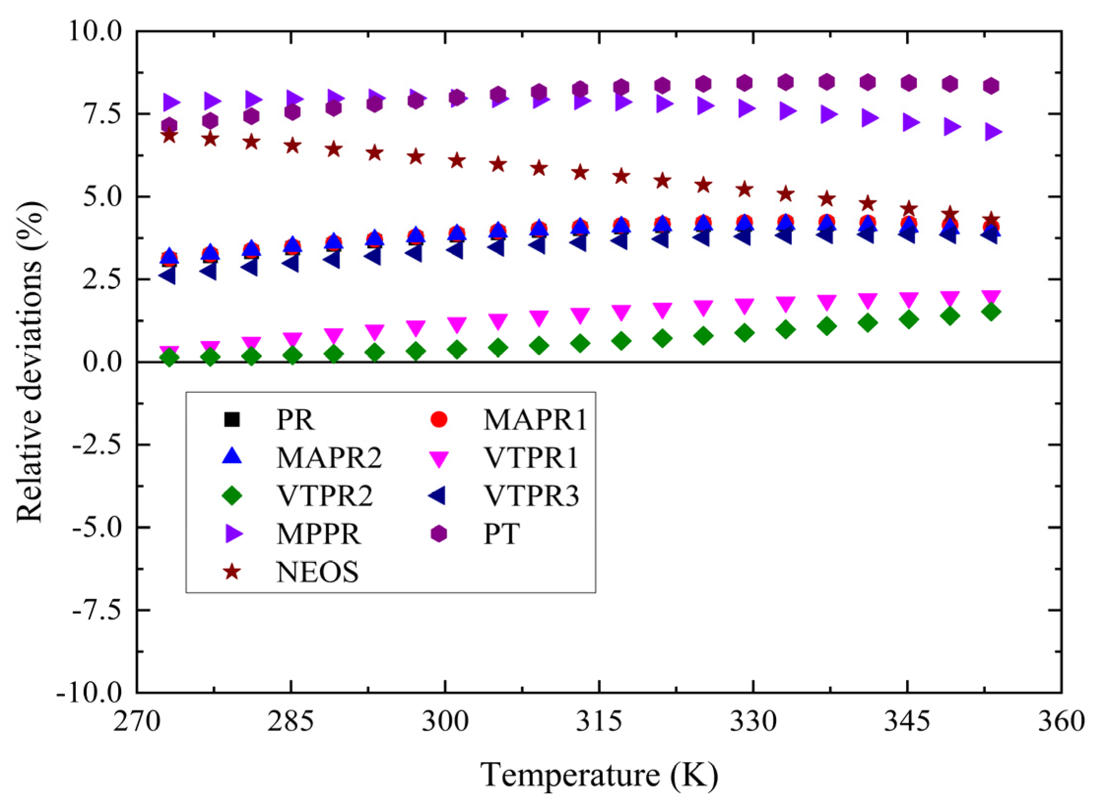
3.2.3. Comparison and Discussion of Different Models of Saturated Vapor Pressure
3.2.4. Comparison and Discussion of Different Models of Saturated Liquid Density
3.3. Prediction Models of Surface Tension
3.3.1. Prediction Models of Surface Tension
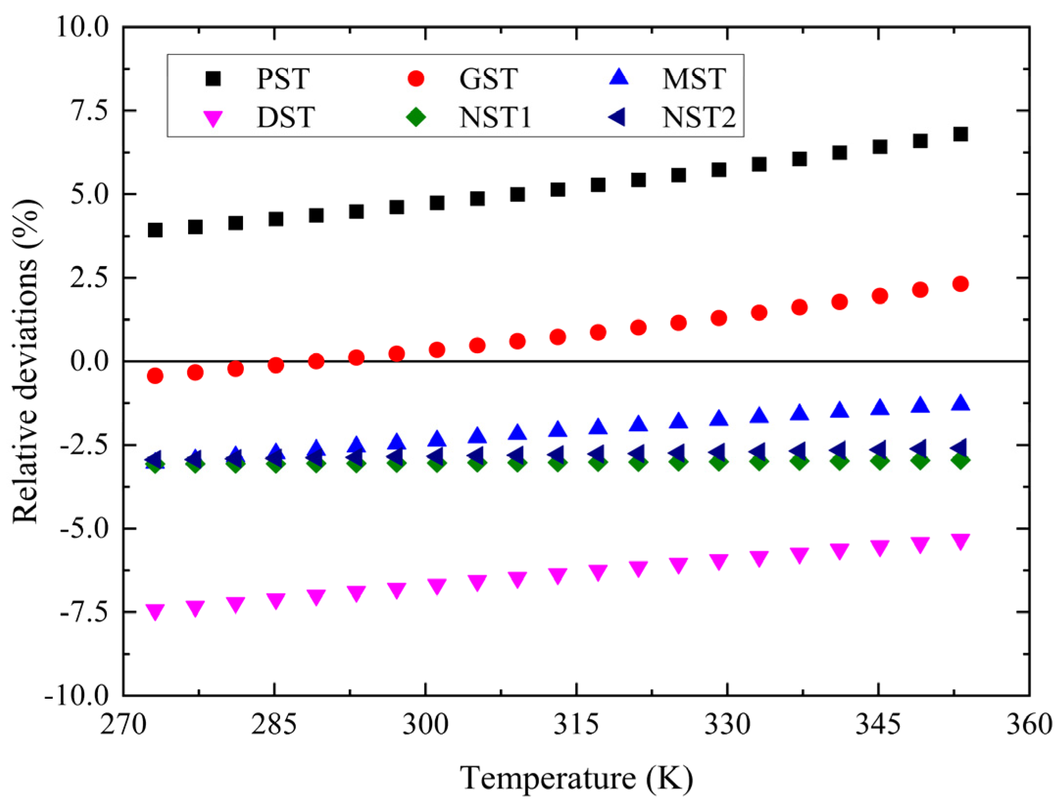
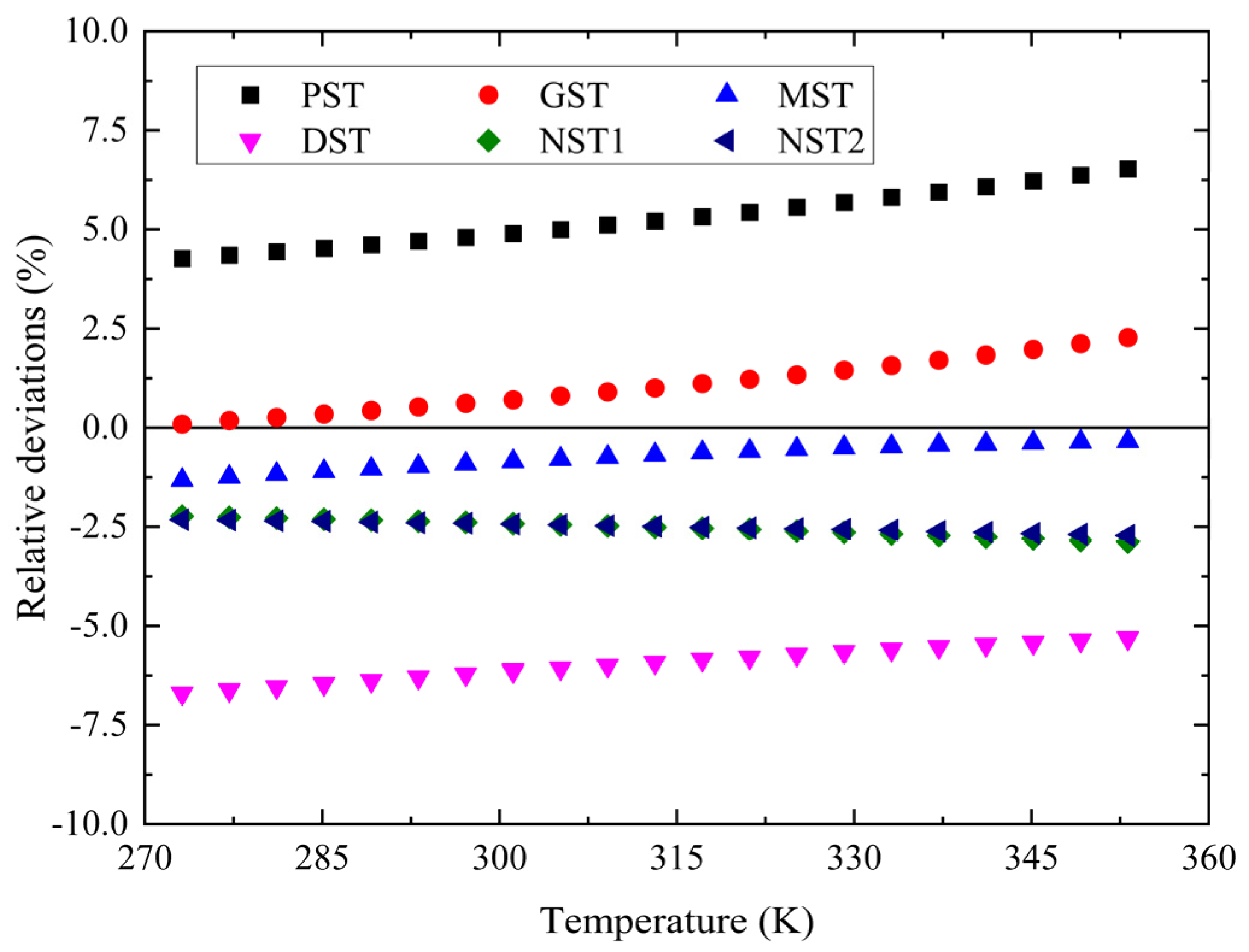
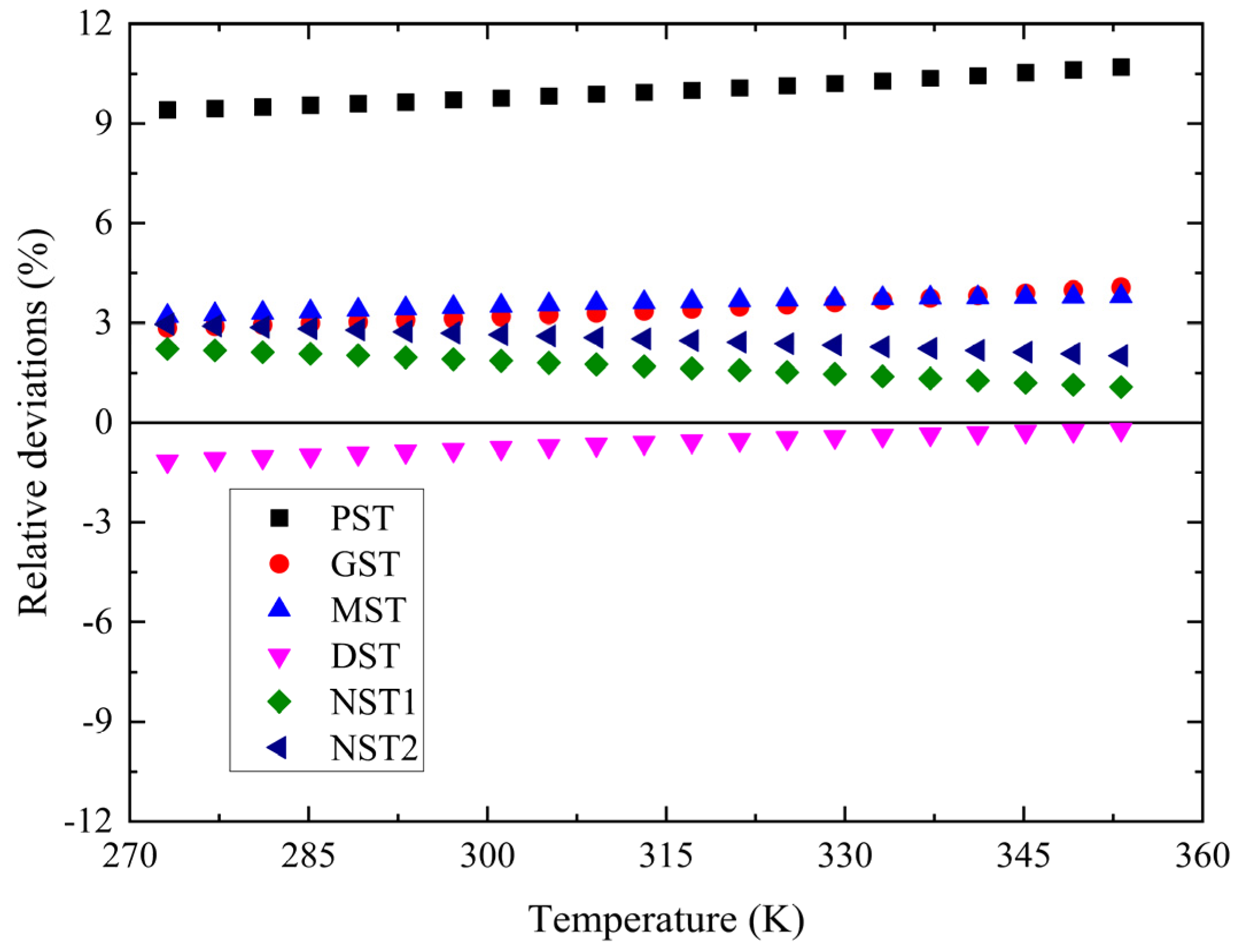
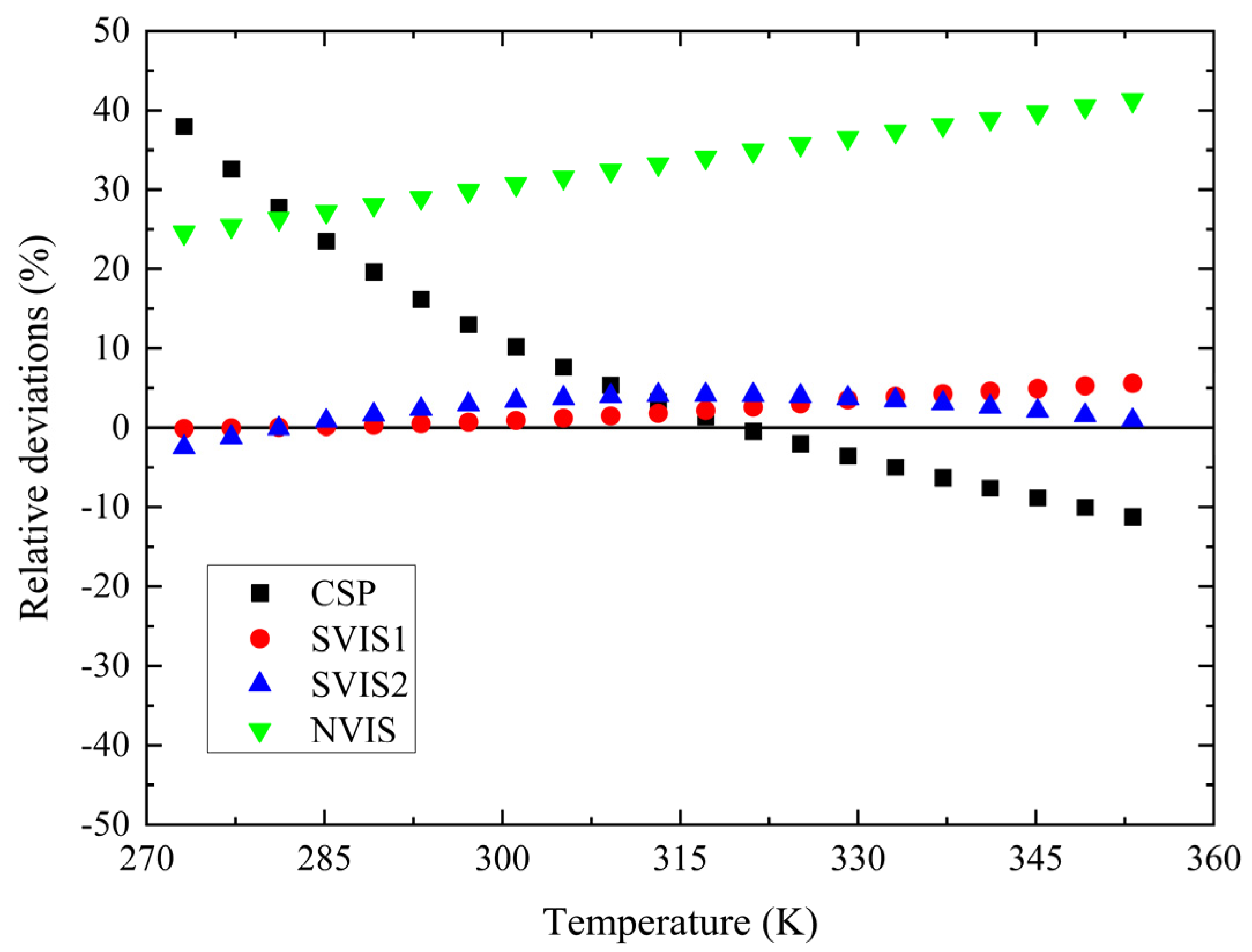
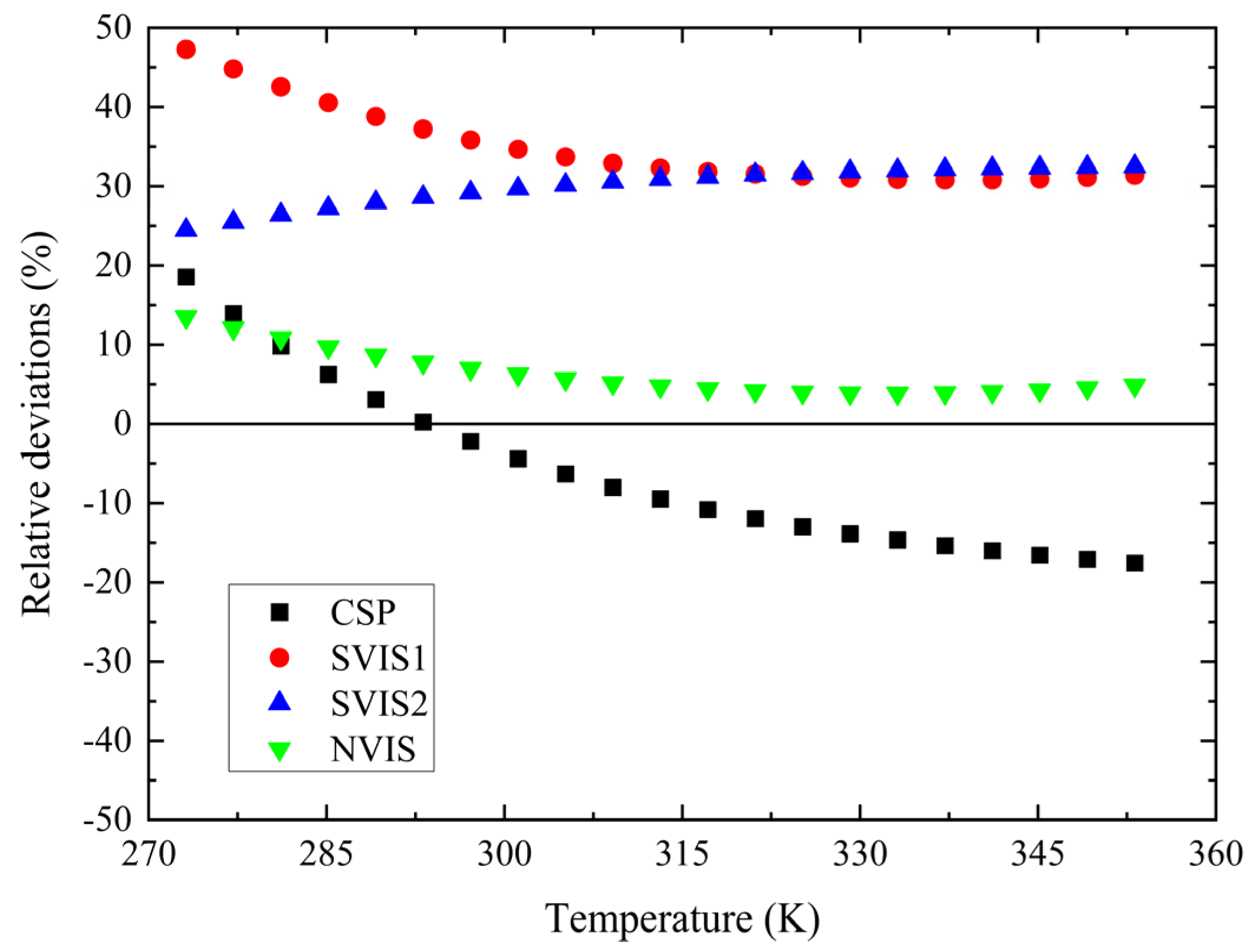
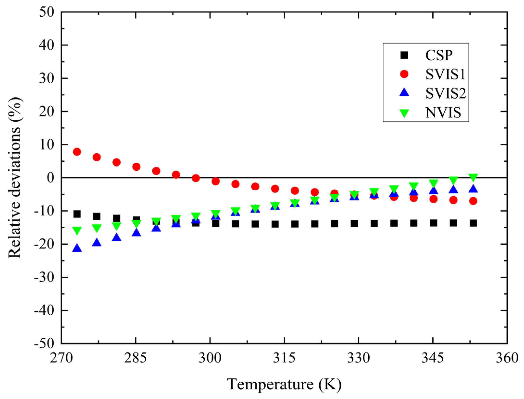
3.3.2. Comparison and Discussion of Different Models of Surface Tension
3.4. Prediction Models of Viscosity and Thermal Conductivity
3.4.1. Prediction Models of Viscosity and Thermal Conductivity
Principle of Corresponding States (PCS)
Other Prediction Models of Viscosity
Other Prediction Models of Thermal Conductivity
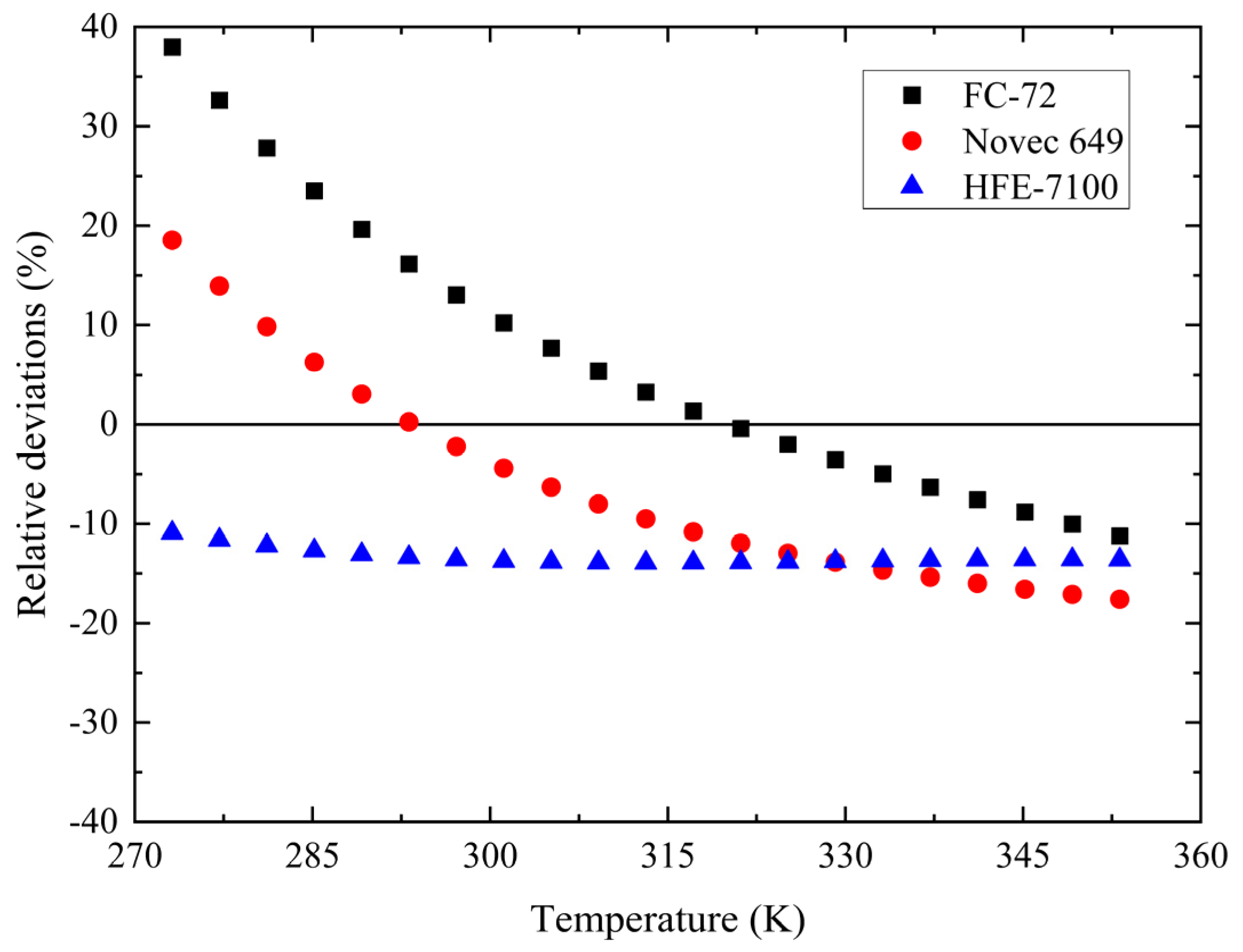
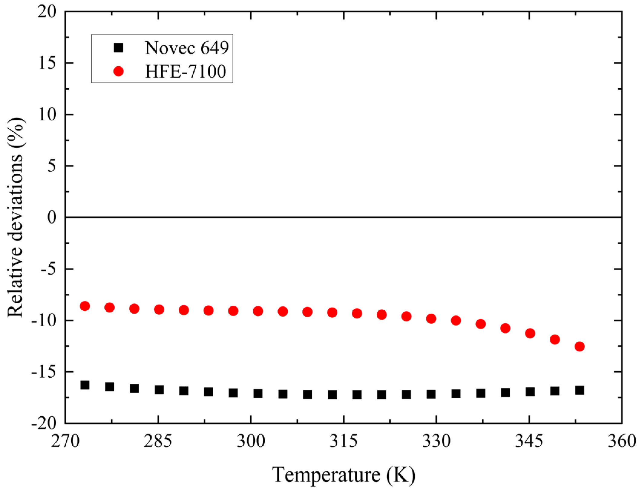
3.4.2. Comparison and Discussion of Different Models of Viscosity and Thermal Conductivity
Discussion of The PCS Model
Comparison and Discussion of Different Models of Viscosity
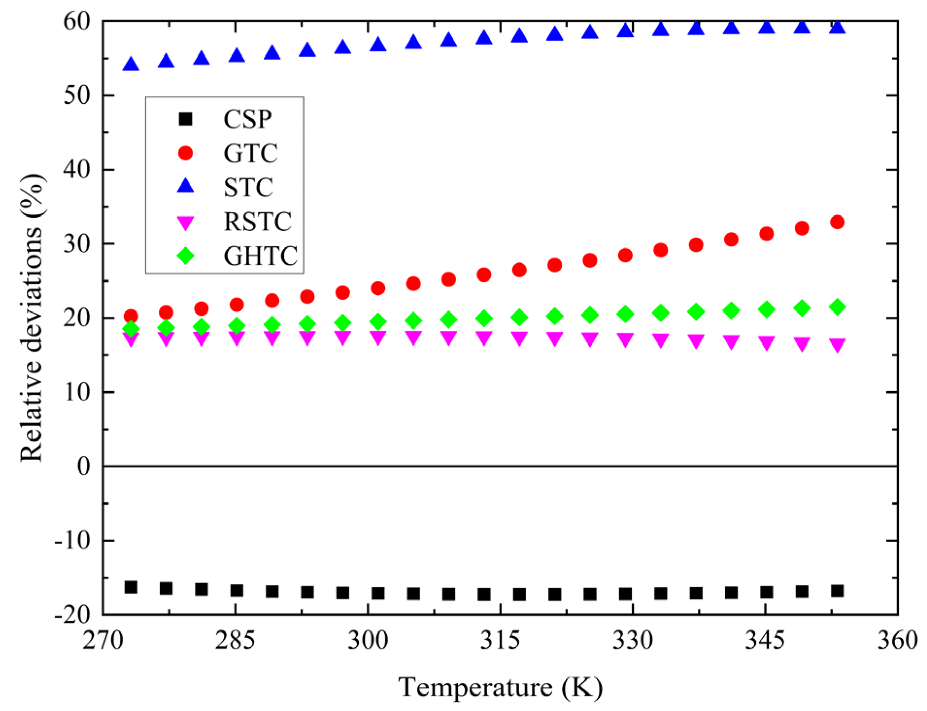
Comparison and Discussion of Different Models of Thermal Conductivity
4. Conclusions
- (1)
- For calculating saturated vapor pressure, the accuracy of the MAPR2 model is best out of all the studied models, while for saturated liquid density, the VTPR2 model has the highest accuracy. Therefore, it is recommended to combine the MAPR2 model and the VTPR2 model to predict the saturated vapor pressure and saturated density of a coolant.
- (2)
- For calculating surface tension, the GST model has a good accuracy for most electronic fluoride liquids, but different models are suitable for fluids with different polarity ranges, which is why the best prediction models for the three coolants are not the same.
- (3)
- For calculating viscosity and thermal conductivity, there were no prediction models with strong versatility and high accuracy found in this work. The effect of fluorine-containing functional groups on the predictive accuracy of viscosity and thermal conductivity of electronic fluoride liquids needs to be further developed.
Author Contributions
Funding
Institutional Review Board Statement
Data Availability Statement
Acknowledgments
Conflicts of Interest
Nomenclature
| Latin alphabet | |||
| a | equation parameters | m | α function coefficient |
| b | equation parameters | M | molar mass (g mol−1) |
| c | equation parameters | NA | Avogadro constant |
| d | equation parameters | p | pressure (Pa) |
| D | diameter (m) | r | radius (m) |
| f | conformal parameters related to temperature | R | gas constant (J mol−1 K−1) |
| F | correction factor | T | temperature (K) |
| g | acceleration of gravity (m s−2) | V | specific volume (m3 kg−1) |
| h | conformal parameters related to density | ΔV | specific volume translation (m3 kg−1) |
| k | Boltzmann constant | Z | compression factor |
| K | coefficient of critical heat flux | CHF | critical heat flux (W m−2) |
| ΔH | latent heat of evaporation (kJ kg−1) | HTC | heat transfer coefficient (W m−2 K−1) |
| Greek alphabet | |||
| α | α function | φ | fugacity coefficient |
| η | dynamic viscosity (Pa s) | χ | correction factor of thermal conductivity |
| κ | hydrogen bonding parameters | ψ | correction factor of viscosity |
| λ | thermal conductivity (W m−1 K−1) | ω | eccentricity factor |
| μ | molecular dipole moment | Ω | collision integral |
| ρ | density (kg m−3) | ξ | theoretical compression factor |
| Subscript | |||
| b | boiling point | r | contrast |
| br | boiling point contrast state | ref | reference |
| c | critical state | s | saturated state |
| dim | dimensionless | V | gas phase |
| L | liquid phase | w | wall |
| o | outside the tube | η | dynamic viscosity |
| PR | PR equation | λ | thermal conductivity |
| pt | pseudo-triple point | 0 | reference fluid |
| Superscript | |||
| int | contribution of intramolecular motion | * | dilution gas item |
References
- Srivastava, A.; Gupta, M.; Kaur, G. Energy efficient transmission trends towards future green cognitive radio networks (5G): Progress, taxonomy and open challenges. J. Netw. Comput. Appl. 2020, 168, 102760. [Google Scholar] [CrossRef]
- Markets and Markets. Digital Transformation Market by Component, Technology (Cloud Computing, Big Data & Analytics, Mobility & Social Medial Management, Cybersecurity, AI), Deployment Mode, Organization Size, Business Function, Vertical and Region—Global Forecast to 2027. 2023. Available online: https://www.marketsandmarkets.com/Market-Reports/digital-transformation-market-43010479.html (accessed on 24 February 2023).
- Ryan, M. Compute Power Is Becoming a Bottleneck for Developing AI. Tech Monitor, UK. 2022. Available online: https://techmonitor.ai/technology/ai-and-automation/chatgpt-ai-compute-power (accessed on 24 February 2023).
- Luo, Y. Will ChatGPT Promote the Domestic Chipherstellers. 21st Century Business Herald, 17 February 2023; 12. [Google Scholar] [CrossRef]
- Zhang, S. ChatGPT drives the development of AI chips. 21st Century Business Herald, 9 February 2023; 9. [Google Scholar] [CrossRef]
- Salahuddin, S.; Ni, K.; Datta, S. The era of hyper-scaling in electronics. Nat. Electron. 2018, 1, 442–450. [Google Scholar] [CrossRef]
- Josh, M. Understanding Data Center Energy Consumption. 2023. Available online: https://alterumtech.com/data-center-energy-consumption/ (accessed on 24 February 2023).
- Nicola, J. How to stop data centres from gobbling up the world’s electricity. Nature 2018, 561, 163–166. [Google Scholar] [CrossRef]
- Mitchell, J.; Koomey, J.; Nordman, B.; Blazek, M. Data center power requirements: Measurements from Silicon Valley. Energy. 2003, 28, 837–850. [Google Scholar] [CrossRef]
- Paul, L.; Tony, D.; Data Center Science Center. Data center science center. White Paper 279: Five reasons to adopt liquid cooling. Schneider Electric. 2019. Available online: https://download.schneider-electric.com/files?p_enDocType=White+Paper&p_File_Name=WP279R0_CH.pdf&p_Doc_Ref=SPD_WTOL-B9RKEA_CH (accessed on 24 February 2023).
- Liu, H.; Wei, Z.; He, W.; Zhao, J. Thermal issues about Li-ion batteries and recent progress in battery thermal management systems: A review. Energy Convers. Manag. 2017, 150, 304–330. [Google Scholar] [CrossRef]
- Bibin, C.; Vijayaram, M.; Suriya, V.; Sai Ganesh, R.; Soundarraj, S. A review on thermal issues in Li-ion battery and recent advancements in battery thermal management system. Mater. Today Proc. 2020, 33, 116–128. [Google Scholar] [CrossRef]
- Wu, X.; Liu, Y.; Ni, H.; Huang, J.; Guo, H.; Zhuang, Y.; Han, X. Effect of different electronic cooling liquid on the performance of immersion phase change cooling system. J. Refrig. 2021, 42, 74–82. [Google Scholar]
- Kheirabadi, A.; Groulx, D. Cooling of server electronics: A design review of existing technology. Appl. Therm. Eng. 2016, 105, 622–638. [Google Scholar] [CrossRef]
- Habibi, K.; Halgamuge, A. A review on efficient thermal management of air- and liquid-cooled data centers: From chip to the cooling system. Appl. Energy 2017, 205, 1165–1188. [Google Scholar] [CrossRef]
- Matsuoka, M.; Matsuda, K.; Kubo, H. Liquid immersion cooling technology with natural convection in data center. In Proceedings of the 2017 IEEE 6th International Conference on Cloud Networking (CloudNet), Prague, Czech Republic, 25–27 September 2017; pp. 101–107. [Google Scholar] [CrossRef]
- Wagner, G.; Schaadt, J.; Dixon, J.; Chan, G.; Copeland, D. Test results from the comparison of three liquid cooling methods for high-power processors. In Proceedings of the IEEE Intersociety Conference on Thermal and Thermomechanical Phenomena in Electronic Systems (ITherm), Las Vegas, NV, USA, 31 May–3 June 2016; pp. 619–624. [Google Scholar] [CrossRef]
- Bai, L.; Zhan, L.; Lin, G.; Peterson, G. Pool boiling with high heat flux enabled by a porous artery structure. Appl. Phys. Lett. 2016, 108, 221602. [Google Scholar] [CrossRef]
- Li, X.; Lv, L.; Wang, X.; Li, J. Transient thermodynamic response and boiling heat transfer limit of dielectric liquids in a two-phase closed direct immersion cooling system. Therm. Sci. Eng. Prog. 2021, 25, 100986. [Google Scholar] [CrossRef]
- Alibaba. Apsara Conference—Apsara Intelligence. 2017. Available online: https://yunqi.aliyun.com/2017/nanjing/index?spm=a2c4e.11165380.747884.5.3aa42d9fOwU6Mi (accessed on 24 February 2023).
- IDCC2021. The 16th China IDC Industry Annual Ceremony. 2021. Available online: http://news.idcquan.com/news/180569.shtml (accessed on 24 February 2023).
- Iceotope. Unlimiting Performance from the Cloud to the Edge. 2022. Available online: https://www.iceotope.com/technologies/ (accessed on 24 February 2023).
- CITE2020. The 8th China Information Technology Expo. 2020. Available online: https://www.citexpo.org/ (accessed on 24 February 2023).
- Sugon. The First Commercial Liquid Immersion Cooling Server in China. 2017. Available online: https://www.sugon.com/cut?id=705&nav_id=48 (accessed on 24 February 2023).
- MarketsandMarkets. Immersion Cooling Market by Type (Single-Phase and Two-Phase), Application (High Performance Computing, Edge Computing, Cryptocurrency Mining), Cooling Fluid Type (Mineral Oil, Synthetic Oil, Fluorocarbon Based), Geography—Global Forecast to 2030. 2023. Available online: https://www.marketsandmarkets.com/Market-Reports/immersion-cooling-market-107040948.html (accessed on 24 February 2023).
- Sebastian, M. GRC Details Immersion Cooling Deployment for the US Air force. 2019. Available online: https://www.datacenterdynamics.com/en/news/grc-details-immersion-cooling-deployment-us-air-force/ (accessed on 24 February 2023).
- GRC. Vienna Scientific Cluster’s—The Immersion Supercomputer: Extreme Efficiency, Needs No Water. 2014. Available online: https://www.grcooling.com/learning-center/vsc-immersion-supercomputer/ (accessed on 24 February 2023).
- GRC. Liquid Immersion Cooling’s Most Effective Coolants. 2018. Available online: https://www.grcooling.com/wp-content/uploads/2018/06/GRC_Fact_Sheet_ElectroSafe.pdf (accessed on 24 February 2023).
- 3M. Two-Phase Immersion Cooling—A Revolution in Data Center Efficiency. 2015. Available online: https://multimedia.3m.com.cn/mws/media/1127920O/2-phase-immersion-coolinga-revolution-in-data-center-efficiency.pdf (accessed on 24 February 2023).
- Xia, L.; Wang, W.; Zhu, Y. Status and trend of millimeter—Wave CMOS integrated circuits. Semicond. Technol. 2007, 223, 197–201. [Google Scholar] [CrossRef]
- Endo, T.; Nukada, A.; Matsuoka, S. TSUBAME-KFC: A modern liquid submersion cooling prototype towards exascale becoming the greenest supercomputer in the world. In Proceedings of the 2014 20th IEEE International Conference on Parallel and Distributed Systems (ICPADS), Hsinchu, China, 16–19 December 2014; pp. 360–367. [Google Scholar] [CrossRef]
- Cooling Loop. 2012. Available online: https://welcolab.wixsite.com/discovery/8-cooling-liquids (accessed on 24 February 2023).
- GRC. The Coolest Answer to Power Hungry Data Centers. 2021. Available online: https://www.grcooling.com/wp-content/uploads/2018/06/GRC_ICE_Product_Brochure.pdf (accessed on 24 February 2023).
- TACC. A Top-20 Supercomputing Facility Rethinks Its Cooling Efficiency with Fluid-Submersion Cooling. 2018. Available online: https://dl.acm.org/action/downloadSupplement?doi=10.1145%2F2148600.2148631&file=post198.pdf (accessed on 24 February 2023).
- Danielson, R.; Krajewski, N.; Brost, J. Cooling a superfast computer. Electron. Packag. Prod. 1986, 26, 44–45. [Google Scholar]
- Zhan, W. A supercomputer system CRAY-2. J. Comput. Res. Deve. 1986, 23, 58–64. [Google Scholar]
- Simons, R. Direct liquid immersion cooling for high power density microelectronics. Electron. Cooling. 1996. Available online: https://www.electronics-cooling.com/1996/05/direct-liquid-immersion-cooling-for-high-power-density-microelectronics/ (accessed on 24 February 2023).
- Li, J. Liquid Cooling Revolution—A Black Technology Transforming the Data Center; Posts Telecom Presse: Beijing, China, 2019. [Google Scholar]
- Wu, X.; Yang, J.; Guo, H.; Zhuang, Y.; Li, C.; Liu, Y.; Han, X. Development history and design of key links in immersion liquid cooling system for data center. Refrig. Air-Cond. 2022, 22, 61–74. [Google Scholar]
- Phoenik. In new infrastructure construction era, immersion cooling will be popular in data centers. Data Center Setup+ 2020, 21, 55–56. [Google Scholar]
- Patrick, K. Sugon Nebula Phase Change Immersion Cooling a Unique Platform. 2018. Available online: https://www.servethehome.com/sugon-nebula-phase-change-immersion-cooling-a-unique-platform/ (accessed on 24 February 2023).
- Peter, J. EcoDataCenter to Deploy Iceotope Immersion Cooling. 2020. Available online: https://www.datacenterdynamics.com/en/news/ecodatacenter-deploy-iceotope-immersion-cooling/ (accessed on 24 February 2023).
- Yang, S.; Tao, W. Heat Transfer, 4th ed.; Higher Education Press: Beijing, China, 2006. [Google Scholar]
- Carey, V. Liquid-Vapor Phase-Change Phenomena: An Introduction to the Thermophysics of Vaporization and Condensation Processes in Heat Transfer Equipment, 2nd ed.; Hemisphere Publishing Corporation: Washington, DC, USA, 1992. [Google Scholar] [CrossRef]
- Wu, X.; Li, C.; Yang, J.; Liu, Y.; Han, X. Theoretical and experimental research on flow boiling heat transfer in microchannels for IGBT modules. Int. J. Heat Mass Transf. 2023, 205, 123900. [Google Scholar] [CrossRef]
- Lienhard, J.; Dhir, V.; Riherd, D. Peak pool boiling heat-flux measurements on finite horizontal flat plates. J. Heat Transf. 1973, 95, 477. [Google Scholar] [CrossRef]
- Dhir, V.; Lienhard, J. Laminar film condensation on plane and axisymmetric bodies in nonuniform gravity. J. Heat Transf. 1971, 93, 97–100. [Google Scholar] [CrossRef]
- Ozmat, B. Interconnect technologies and the thermal performance of MCM. In [1992 Proceedings] Intersociety Conference on Thermal Phenomena in Electronic Systems; IEEE: Austin, TX, USA, 1992; pp. 226–245. [Google Scholar] [CrossRef]
- Shah, A. Exergy-Based Analysis and Optimization of Computer Thermal Management Systems; University of California Berkeley: Berkeley, CA, USA, 2005. [Google Scholar]
- GRC. ElectrosafeTM Plus-Safety Data Sheet. 2017. Available online: https://www.forvice.co.jp/wp/wp-content/uploads/%E2%97%86Electrosafe-Plus-SDS.pdf (accessed on 24 February 2023).
- GRC. ElectroSafeTM Dielectric Liquid Coolant. 2018. Available online: https://www.grcooling.com (accessed on 24 February 2023).
- El-Genk, M. Immersion cooling nucleate boiling of high power computer chips. Energy Convers. Manag. 2012, 53, 205–218. [Google Scholar] [CrossRef]
- Gess, J.; Bhavnani, S.; Ramakrishnan, B.; Johnson, R.; Harris, D.; Knight, R.; Hamilton, M.; Ellis, C. Impact of surface enhancements upon boiling heat transfer in a liquid immersion cooled high performance small form factor server model. In Proceedings of the 14th Intersociety Conference on Thermal and Thermomechanical Phenomena in Electronic Systems (ITherm), Orlando, FL, USA, 27–30 May 2014; pp. 435–443. [Google Scholar] [CrossRef]
- Hsu, Y.; Li, J.; Lu, M. Enhanced immersion cooling using two-tier micro- and nano-structures. Appl. Therm. Eng. 2018, 131, 864–873. [Google Scholar] [CrossRef]
- Lee, J.; Mudawar, I. Fluid flow and heat transfer characteristics of low temperature two-phase micro-channel heat sinks—Part 1: Experimental methods and flow visualization results. Int. J. Heat Mass Transf. 2008, 51, 4315–4326. [Google Scholar] [CrossRef]
- Lee, J.; Mudawar, I. Fluid flow and heat transfer characteristics of low temperature two-phase micro-channel heat sinks—Part 2. Subcooled boiling pressure drop and heat transfer. Int. J. Heat Mass Transf. 2008, 51, 4327–4341. [Google Scholar] [CrossRef]
- Yoon, Y.; Yang, H.; Kwak, H. Enhancement of the critical heat flux by using heat spreader. KSME Int. J. 2003, 17, 1063–1072. [Google Scholar] [CrossRef]
- Stiles, V.; Cady, G. Physical properties of perfluoro-n-hexane and perfluoro-2-methylpentane. J. Am. Chem. Soc. 1952, 74, 3771–3773. [Google Scholar] [CrossRef]
- Dunlap, R.; Murphy, C.; Bedford, R. Some physical properties of perfluoro-n-hexane. J. Am. Chem. Soc. 1958, 80, 83–85. [Google Scholar] [CrossRef]
- Dias, A.; Gonçalves, C.; Caço, A.; Santos, L.; Piñeiro, M.; Vega, L.; Coutinho, J.; Marrucho, I. Densities and vapor pressures of highly fluorinated compounds. J. Chem. Eng. Data 2005, 50, 1328–1333. [Google Scholar] [CrossRef]
- Freire, M.; Ferreira, A.; Fonseca, I.; Marrucho, I.; Coutinho, J. Viscosities of liquid fluorocompounds. J. Chem. Eng. Data 2008, 53, 538–542. [Google Scholar] [CrossRef] [Green Version]
- Freire, M.; Carvalho, P.; Queimada, A.; Marrucho, I.; Coutinho, J. Surface tension of liquid fluorocompounds. J. Chem. Eng. Data 2006, 51, 1820–1824. [Google Scholar] [CrossRef]
- Cochran, M.; North, A.; Pethrick, R. Ultrasonic studies of perfluoro-n-alkanes. J. Am. Chem. Soc. Faraday Trans. 1974, 70, 1274–1279. [Google Scholar] [CrossRef]
- Morgado, P.; Laginhas, C.; Lewis, J.; McCabe, C.; Martins, L.; Filipe, E. Viscosity of liquid perfluoroalkanes and perfluoroalkylalkane surfactants. J. Phys. Chem. B 2011, 115, 9130–9139. [Google Scholar] [CrossRef] [PubMed] [Green Version]
- Irving, J.; Jamieson, D. Thermal conductivity of 13 fluorocarbon liquids. J. Fluor. Chem. 1975, 5, 449–456. [Google Scholar] [CrossRef]
- McLinden, M.; Perkins, R.; Lemmon, E.; Fortin, T. Thermodynamic properties of 1,1,1,2,2,4,5,5,5-nonafluoro-4-(trifluoromethyl)-3-pentanone: Vapor pressure, (p, ρ, t) behavior, and speed of sound measurements, and an equation of state. J. Chem. Eng. Data 2015, 60, 3646–3659. [Google Scholar] [CrossRef]
- Tanaka, K. Measurement of pρT Properties of 1,1,1,2,2,4,5,5,5-Nonafluoro-4-(trifluoromethyl)-3-pentanone in the Near-Critical and Supercritical Regions. J. Chem. Eng. Data 2016, 61, 3958–3961. [Google Scholar] [CrossRef]
- Perkins, R.; Huber, M.; Assael, M. Measurement and correlation of the thermal conductivity of 1,1,1,2,2,4,5,5,5-nonafluoro-4-(trifluoromethyl)-3-pentanone. J. Chem. Eng. Data 2018, 63, 2783–2789. [Google Scholar] [CrossRef]
- Wen, C.; Meng, X.; Huber, M.; Wu, J. Measurement and correlation of the viscosity of 1,1,1,2,2,4,5,5,5-nonafluoro-4-(trifluoromethyl)-3-pentanone. J. Chem. Eng. Data 2017, 62, 3603–3609. [Google Scholar] [CrossRef] [PubMed]
- Cui, J.; Yan, S.; Bi, S.; Wu, J. Saturated liquid dynamic viscosity and surface tension of trans-1-chloro-3,3,3-trifluoropropene and dodecafluoro-2-methylpentan-3-one. J. Chem. Eng. Data 2018, 63, 751–756. [Google Scholar] [CrossRef]
- Rausch, M.; Kretschmer, L.; Will, S.; Leipertz, A.; Fröba, A. Density, surface tension, and kinematic viscosity of hydrofluoroethers HFE-7000, HFE-7100, HFE-7200, HFE-7300, and HFE-7500. J. Chem. Eng. Data 2015, 60, 3759–3765. [Google Scholar] [CrossRef]
- Bi, S.; Cui, J.; Ma, L.; Zhao, G.; Wu, J. Thermophysical properties of HFE7100 and HFE7500. CIESC J. 2016, 67, 1680–1686. [Google Scholar]
- An, B.; Duan, Y.; Tan, L.; Yang, Z. Vapor pressure of HFE 7100. J. Chem. Eng. Data 2015, 60, 1206–1210. [Google Scholar] [CrossRef]
- Meng, X.; Wei, K.; Wu, J. Viscosity measurements for two new working fluids of HFE-7000 and HFE-7100. Sci. Paper Online 2014. Available online: http://www.paper.edu.cn/releasepaper/content/201401-1259 (accessed on 24 February 2023).
- Piñeiro, M.; Bessières, D.; Legido, J.; Saint-Guirons, H. PρT measurements of nonafluorobutyl methyl ether and nonafluorobutyl ethyl ether between 283.15 and 323.15 K at pressures up to 40 MPa. Int. J. Thermophys. 2003, 24, 1265–1276. [Google Scholar] [CrossRef]
- An, B.; Tan, L.; Duan, Y.; Yang, Z. PvT properties for R-227ea and HFE-7100 in the liquid phase. J. Chem. Eng. Data 2016, 61, 1462–1467. [Google Scholar] [CrossRef]
- Li, X.; Bi, S.; Zhao, G.; Lu, P.; Wang, Y. Experiment on liquid density and surface tension of nonafluorobutylmethylether. J. Xi’an Jiaotong Univ. 2011, 45, 70–73. [Google Scholar]
- Qi, H.; Fang, D.; Meng, X.; Wu, J. Liquid density of HFE-7000 and HFE-7100 from T = (283 to 363) K at pressures up to 100 MPa. J. Chem. Thermodyn. 2014, 77, 131–136. [Google Scholar] [CrossRef]
- Hu, X.; Meng, X.; Wei, K.; Li, W.; Wu, J. Compressed liquid viscosity measurements of HFE-7000, HFE-7100, HFE-7200, and HFE-7500 at temperatures from (253 to 373) K and pressures up to 30 MPa. J. Chem. Eng. Data 2015, 60, 3562–3570. [Google Scholar] [CrossRef]
- Zheng, Y.; Wei, Z.; Song, X. Measurements of isobaric heat capacities for HFE-7000 and HFE-7100 at different temperatures and pressures. Fluid Phase Equilibria 2016, 425, 335–341. [Google Scholar] [CrossRef]
- Chen, X.; Cai, Z.; Qian, C. Chemical Engineering Thermodynamics, 5th ed.; Chemical Industry Press Co., Ltd.: Beijing, China, 2020. [Google Scholar]
- Tanaka, K.; Ishikawa, J.; Kontomaris, K. Thermodynamic properties of HFO-1336mzz(E) (trans-1,1,1,4,4,4-hexafluoro-2-butene) at saturation conditions. Int. J. Refrig. 2017, 82, 283–287. [Google Scholar] [CrossRef]
- Lemmon, E.; Bell, I.; Huber, M. NIST standard reference database; Version 10.0 REFPROP; National Institute of Standards and Technology: Gaithersburg, MD, USA, 2018.
- Vandana, V.; Rosenthal, D.; Teja, A. The critical properties of perfluoro n-alkanes. Fluid Phase Equilibria 1994, 99, 209–218. [Google Scholar] [CrossRef]
- 3M. 3MTM NovecTM 649 Engineered Fluid. 2019. Available online: https://www.3m.com (accessed on 24 February 2023).
- Peng, D.; Robinson, D. A new two-constant equation of state. Ind. Eng. Chem. Fundam. 1976, 15, 59–64. [Google Scholar] [CrossRef]
- Lin, H.; Duan, Y. Density correction of the peng-robinson equation of state for halogenated hydrocarbons. J. Eng. Thermophys. 2006, 27, 13–16. [Google Scholar]
- Duan, Y.; Lin, H. Modified cubic equations of state by volumetranslation method. In Proceedings of the 4th Chian New Technology of Refrigeration and air Conditioning Conference, Nanjing, China, 9–11 April 2006; p. 7. [Google Scholar]
- Pina-Martinez, A.; Privat, R.; Jaubert, J.; Peng, D. Updated versions of the generalized Soave α-function suitable for the Redlich-Kwong and Peng-Robinson equations of state. Fluid Phase Equilibria 2019, 485, 264–269. [Google Scholar] [CrossRef]
- Lopez-Echeverry, J.; Reif-Acherman, S.; Araujo-Lopez, E. Peng-Robinson equation of state: 40 years through cubics. Fluid Phase Equilibria 2017, 447, 39–71. [Google Scholar] [CrossRef]
- Forero, G.L.; Velásquez, J. The Patel–Teja and the Peng–Robinson EoSs performance when Soave alpha function is replaced by an exponential function. Fluid Phase Equilibria 2012, 332, 55–76. [Google Scholar] [CrossRef]
- Kumar, A.; Okuno, R. Critical parameters optimized for accurate phase behavior modeling for heavy n-alkanes up to C100 using the Peng–Robinson equation of state. Fluid Phase Equilibria 2012, 335, 46–59. [Google Scholar] [CrossRef]
- Nazarzadeh, M.; Moshfeghian, M. New volume translated PR equation of state for pure compounds and gas condensate systems. Fluid Phase Equilibria 2013, 337, 214–223. [Google Scholar] [CrossRef]
- Haghtalab, A.; Mahmoodi, P.; Mazloumi, S. A modified Peng–Robinson equation of state for phase equilibrium calculation of liquefied, synthetic natural gas, and gas condensate mixtures. Can. J. Chem. Eng. 2011, 89, 1376–1387. [Google Scholar] [CrossRef]
- Tong, J. Thermophysical Properties of Fluids; China Petrochemical Press: Beijing, China, 1996. [Google Scholar]
- Martin, J. Cubic equations of state-which. Ind. Eng. Chem. Fundam. 1979, 18, 81–97. [Google Scholar] [CrossRef]
- Nasrifar, K.; Moshfeghian, M. A new cubic equation of state for simple fluids: Pure and mixture. Fluid Phase Equilibria 2001, 190, 73–88. [Google Scholar] [CrossRef]
- Haghtalab, A.; Kamali, M.; Mazloumi, S.; Mahmoodi, P. A new three-parameter cubic equation of state for calculation physical properties and vapor–liquid equilibria. Fluid Phase Equilibria 2010, 293, 209–218. [Google Scholar] [CrossRef]
- Brock, J.; Bird, R. Surface tension and the principle of corresponding states. AIChE J. 1955, 1, 174–177. [Google Scholar] [CrossRef]
- Pitzer, K. Thermodynamics; McGraw-Hill: New York, NY, USA, 1995. [Google Scholar]
- Gharagheizi, F.; Eslamimanesh, A.; Sattari, M.; Mohammadi, A.; Richon, D. Development of corresponding states model for estimation of the surface tension of chemical compounds. AIChE J. 2013, 59, 613–621. [Google Scholar] [CrossRef]
- Miqueu, C.; Broseta, D.; Satherley, J.; Mendiboure, B.; Lachaise, J.; Graciaa, A. An extended scaled equation for the temperature dependence of the surface tension of pure compounds inferred from an analysis of experimental data. Fluid Phase Equilibria 2000, 172, 169–182. [Google Scholar] [CrossRef]
- Schmidt, J.; Carrillo-Nava, E.; Moldover, M. Partially halogenated hydrocarbons CHFCl-CF3, CF3-CH3, CF3-CHF-CHF2, CF3-CH2-CF3, CHF2-CF2-CH2F, CF3-CH2-CHF2, CF3-O-CHF2: Critical temperature, refractive indices, surface tension and estimates of liquid, vapor and critical densities. Fluid Phase Equilibria 1996, 122, 187–206. [Google Scholar] [CrossRef]
- Duan, Y.; Zhang, C.; Lin, H.; Zhu, M. The prediction of surface tension for HFCs and HCFCs. J. Eng. Thermophys. 2001, 22, 278–280. [Google Scholar]
- Nicola, G.; Nicola, C.; Moglie, M. A new surface tension equation for refrigerants. Int. J. Thermophys. 2013, 34, 2243–2260. [Google Scholar] [CrossRef]
- Nicola, G.; Moglie, M. A generalized equation for the surface tension of refrigerants. Int. J. Thermophys. 2011, 34, 1098–1108. [Google Scholar] [CrossRef]
- Huber, M. Models for Viscosity, Thermal Conductivity, and Surface Tension of Selected Pure Fluids as Implemented in REFPROP v10.0; National Institute of Standards and Technology: Gaithersburg, MD, USA, 2018.
- Chen, X.; Hou, Y. A new version of the shape factor corresponding states principle. J. Chem. Engin. Chin. Univ. 1993, 7, 296–303. [Google Scholar]
- Ghosh, T.; Prasad, D.; Dutt, N.; Rani, K. Viscosity of Liquids: Theory, Estimation, Experiment, and Data, Viscosity of Liquids: Theory, Estimation, Experiment, and Data; Springer: Berlin, Germany, 2007; Available online: https://link.springer.com/content/pdf/bfm:978-1-4020-5482-2/1.pdf (accessed on 24 February 2023).
- Sastri, S.; Rao, K. A new group contribution method for predicting viscosity of organic liquids. Chem. Eng. J. 1992, 50, 9–25. [Google Scholar] [CrossRef]
- Sastri, S.; Rao, K. A new method for predicting saturated liquid viscosity at temperatures above the normal boiling point. Fluid Phase Equilibria 2000, 175, 311–323. [Google Scholar] [CrossRef]
- Nannoolal, Y.; Rarey, J.; Ramjugernath, D. Estimation of pure component properties, Part 4: Estimation of the saturated liquid viscosity of non-electrolyte organic compounds via group contributions and group interactions. Fluid Phase Equilibria 2009, 281, 97–119. [Google Scholar] [CrossRef]
- Govender, O.; Rarey, J.; Ramjugernath, D. Estimation of pure component properties, Part 5: Estimation of the thermal conductivity of nonelectrolyte organic liquids via group contributions. J. Chem. Eng. Data 2020, 65, 1300–1312. [Google Scholar] [CrossRef]
- Latini, G.; Nicola, G.; Pierantozzi, M. A method to estimate the thermal conductivity of organic alcohols in the liquid phase at atmospheric pressure or along the saturation line. Fluid Phase Equilibria 2016, 427, 488–497. [Google Scholar] [CrossRef]
- Sastri, S.; Rao, K. A new temperature—Thermal conductivity relationship for predicting saturated liquid thermal conductivity. Chem. Eng. J. 1999, 74, 161–169. [Google Scholar] [CrossRef]
- Latini, G.; Sotte, M. Thermal conductivity of refrigerants in the liquid state: A comparison of estimation methods. Int. J. Refrig. 2012, 35, 1377–1383. [Google Scholar] [CrossRef]
- Gharagheizi, F.; Ilani-Kashkouli, P.; Sattari, M.; Mohammadi, A.; Ramjugernath, D.; Richon, D. Development of a general model for determination of thermal conductivity of liquid chemical compounds at atmospheric pressure. AIChE J. 2013, 59, 1702–1708. [Google Scholar] [CrossRef]
- Krauss, R.; Luettmer-Strathmann, J.; Sengers, J.; Stephan, K. Transport properties of 1,1,1,2-tetrafluoroethane (R134a). Int. J. Thermophys. 1993, 14, 951–988. [Google Scholar] [CrossRef]
- Huber, M.; Laesecke, A.; Perkins, R. Model for the viscosity and thermal conductivity of refrigerants, including a new correlation for the viscosity of R134a. Ind. Eng. Chem. Res. 2003, 42, 3163–3178. [Google Scholar] [CrossRef]
- Velzen, D.; Wang, S. Correlation of viscosity-temperature-chemical structure of organic compound liquid. Chem. Eng. 1974, 4, 60–66. [Google Scholar]
- Marrero, J.; Gani, R. Group-contribution based estimation of pure component properties. Fluid Phase Equilibria 2001, 183–184, 183–208. [Google Scholar] [CrossRef]
- Langmuir, I. Third Colloid Symposium. In Monograph; Chemical Catalog Co.: New York, NY, USA, 1925. [Google Scholar]
- Su, W.; Zhao, L.; Deng, S. Group contribution methods in thermodynamic cycles: Physical properties estimation of pure working fluids. Renew. Sustain. Energy Rev. 2017, 79, 984–1001. [Google Scholar] [CrossRef]


| Reference | Thermophysical Properties | Temperature Range | Pressure Range | Measurement Method or Instrument |
|---|---|---|---|---|
| FC-72 | ||||
| Stiles et al. [58] | Density | 273~323 K | Pycnometer | |
| Saturated vapor Pressure | 284~343 K | |||
| Surface tension | 283~323 K | Capillary ascending method | ||
| Viscosity | 273~323 K | Ubbelohde viscometer | ||
| Dunlap et al. [59] | Saturated vapor Pressure | 303~330 K | Static method | |
| Density | 288~318 K | Atmospheric pressure, saturated state | Expansion bottle | |
| Dias et al. [60] | Saturated vapor pressure | 288~308 K | Static method | |
| Density | 288~298 K | Vibrating tube method | ||
| Freire et al. [61] | Viscosity | 298~318 K | Atmospheric pressure | Ubbelohde viscometer |
| Freire et al. [62] | Surface tension | 283~308 K | Surface pressure gauge | |
| Cochran [63] | Density | 233~253 K | Pycnometer method | |
| Viscosity | 233~253 K | Ubbelohde viscometer | ||
| Specific heat capacity | 233~253 K | Differential scanning calorimeter | ||
| Morgado et al. [64] | Viscosity | 278~323 K | Atmospheric pressure | Ubbelohde viscometer |
| Irving et al. [65] | Thermal conductivity | 273~318 K | Steady state hot wire method | |
| Novec 649 | ||||
| Mclinden et al. [66] | Saturated vapor pressure | 325~420 K | Static method | |
| Mclinden et al. [66] | Density | 225~470 K | ~25 MPa | Two-sinker density meter |
| Tanaka et al. [67] | Density | 333~523 K | ~10 MPa | Equal volume method |
| Perkins et al. [68] | Thermal conductivity | 183~501 K | ~69 MPa | Transient hot wire method |
| Wen et al. [69] | Viscosity | 243~373 K | ~40 MPa | Vibrating string method |
| Cui et al. [70] | Viscosity | 303~433 K | Surface light scattering method | |
| Surface tension | 303~433 K | Surface light scattering method | ||
| HFE-7100 | ||||
| Rausch et al. [71] | Density | 273~363 K | Vibrating tube method | |
| Viscosity | 273~373 K | Surface light scattering method | ||
| Surface tension | 273~373 K | Surface light scattering method | ||
| Bi et al. [72] | Thermal conductivity | 252~333 K | Atmospheric pressure | Transient hot wire method |
| Viscosity | 293~393 K | Surface light scattering method | ||
| Surface tension | 293~393 K | Surface light scattering method | ||
| An et al. [73] | Saturated vapor pressure | 306~431 K | Burnett method | |
| Meng et al. [74] | Viscosity | 253~363 K | ~30 MPa | Vibrating string method |
| Piñeiro et al. [75] | Density | 283~323 K | ~40 MPa | Vibrating tube method |
| An et al. [76] | Density | 275~303 K | ~19 MPa | Equal volume method |
| Li et al. [77] | Density | 279~321 K | Atmospheric pressure | Density meter |
| Surface tension | 279~321 K | Capillary ascending method | ||
| Qi et al. [78] | Density | 283~363 K | ~100 MPa | Vibrating tube method |
| Hu et al. [79] | Viscosity | 253~373 K | ~30 MPa | Vibrating string method |
| Zheng et al. [80] | Specific heat capacity | 253~323 K | ~15 MPa | Flow calorimeter |
| Working Fluid | FC-72 | Novec 649 | HFE-7100 |
|---|---|---|---|
| Molecular structure |  |  |  |
| CAS # | 355-42-0 | 756-13-8 | 163702-08-7 |
| Molar mass (g/mol) | 338.04 [83] | 316.04 [69] | 250 [71] |
| Critical temperature (K) | 451.4 [84] | 441.81 [69] | 468.45 [71] |
| Critical pressure (kPa) | 1859 [84] | 1869 [69] | 2230 [71] |
| Critical density (kg/m3) | 621 [84] | 606.81 [69] | 555 [71] |
| Eccentricity factor | 0.486 [83] | 0.471 [69] | 0.436 [77] |
| Dipole moment | 0 [83] | 0.43 [69] | 2.4 [71] |
| Boiling point (K) | 330.27 [83] | 322.15 [85] | 333.15 [77] |
| Model | Expressions | Equation Parameters |
|---|---|---|
| PR | ||
| MAPR1 | ||
| MAPR2 | ||
| VTPR1 | ||
| VTPR2 | ||
| VTPR3 | ||
| MPPR | ||
| PT | ||
| NEOS |
| Model | FC |
|---|---|
| PT | |
| NEOS | |
| Other models |
| Electronic Fluoride Liquid | PR | MAPR1 | MAPR2 | MPPR | PT | NEOS | |
|---|---|---|---|---|---|---|---|
| FC-72 | ARD (%) | 1.03 | 0.60 | 0.26 | 0.36 | 1.39 | 4.44 |
| MRD (%) | 3.57 | 1.65 | 1.07 | 0.69 | 1.93 | 5.22 | |
| Novec 649 | ARD (%) | 0.98 | 0.92 | 0.40 | 0.56 | 1.62 | 4.07 |
| MRD (%) | 3.61 | 1.94 | 1.66 | 1.25 | 2.29 | 4.49 | |
| HFE-7100 | ARD (%) | 1.22 | 1.06 | 0.58 | 0.82 | 1.49 | 2.29 |
| MRD (%) | 5.80 | 4.02 | 3.32 | 3.37 | 3.79 | 4.02 | |
| Electronic Fluoride Liquid | PR | MAPR1 | MAPR2 | VTPR1 | VTPR2 | VTPR3 | MPPR | PT | NEOS | |
|---|---|---|---|---|---|---|---|---|---|---|
| FC-72 | ARD (%) | 3.74 | 3.81 | 3.77 | 1.00 | 0.41 | 3.06 | 8.64 | 9.60 | 2.95 |
| MRD (%) | 4.19 | 4.25 | 4.23 | 1.34 | 0.65 | 3.44 | 9.69 | 10.06 | 3.93 | |
| Novec 649 | ARD (%) | 2.99 | 3.05 | 3.00 | 2.67 | 1.67 | 4.32 | 7.25 | 8.35 | 2.82 |
| MRD (%) | 3.28 | 3.34 | 3.31 | 2.85 | 2.33 | 4.55 | 8.36 | 8.64 | 4.09 | |
| HFE-7100 | ARD (%) | 3.86 | 3.91 | 3.87 | 1.35 | 0.67 | 3.47 | 7.72 | 8.07 | 5.68 |
| MRD (%) | 4.17 | 4.23 | 4.17 | 2.00 | 1.52 | 3.86 | 7.98 | 8.47 | 6.85 | |
| Name | Model Expression |
|---|---|
| PST | |
| GST | |
| MST | |
| DST | |
| NST1 | |
| NST2 |
| Electronic Fluoride Fluid | PST | GST | MST | DST | NST1 | NST2 | |
|---|---|---|---|---|---|---|---|
| FC-72 | ARD (%) | 5.22 | 0.91 | 2.12 | 6.37 | 3.02 | 2.78 |
| MRD (%) | 6.80 | 2.32 | 3.04 | 7.44 | 3.07 | 2.94 | |
| Novec 649 | ARD (%) | 5.28 | 1.07 | 0.74 | 5.95 | 2.53 | 2.50 |
| MRD (%) | 6.53 | 2.27 | 1.32 | 6.70 | 2.88 | 2.72 | |
| HFE-7100 | ARD (%) | 9.98 | 3.39 | 3.57 | 0.64 | 1.67 | 2.51 |
| MRD (%) | 10.70 | 4.07 | 3.80 | 1.16 | 2.22 | 2.96 | |
Disclaimer/Publisher’s Note: The statements, opinions and data contained in all publications are solely those of the individual author(s) and contributor(s) and not of MDPI and/or the editor(s). MDPI and/or the editor(s) disclaim responsibility for any injury to people or property resulting from any ideas, methods, instructions or products referred to in the content. |
© 2023 by the authors. Licensee MDPI, Basel, Switzerland. This article is an open access article distributed under the terms and conditions of the Creative Commons Attribution (CC BY) license (https://creativecommons.org/licenses/by/4.0/).
Share and Cite
Wu, X.; Huang, J.; Zhuang, Y.; Liu, Y.; Yang, J.; Ouyang, H.; Han, X. Prediction Models of Saturated Vapor Pressure, Saturated Density, Surface Tension, Viscosity and Thermal Conductivity of Electronic Fluoride Liquids in Two-Phase Liquid Immersion Cooling Systems: A Comprehensive Review. Appl. Sci. 2023, 13, 4200. https://doi.org/10.3390/app13074200
Wu X, Huang J, Zhuang Y, Liu Y, Yang J, Ouyang H, Han X. Prediction Models of Saturated Vapor Pressure, Saturated Density, Surface Tension, Viscosity and Thermal Conductivity of Electronic Fluoride Liquids in Two-Phase Liquid Immersion Cooling Systems: A Comprehensive Review. Applied Sciences. 2023; 13(7):4200. https://doi.org/10.3390/app13074200
Chicago/Turabian StyleWu, Xilei, Jiongliang Huang, Yuan Zhuang, Ying Liu, Jialiang Yang, Hongsheng Ouyang, and Xiaohong Han. 2023. "Prediction Models of Saturated Vapor Pressure, Saturated Density, Surface Tension, Viscosity and Thermal Conductivity of Electronic Fluoride Liquids in Two-Phase Liquid Immersion Cooling Systems: A Comprehensive Review" Applied Sciences 13, no. 7: 4200. https://doi.org/10.3390/app13074200