Article

Mechanical Response Analysis for an Active–Passive Pile Adjacent to Surcharge Load

1
School of Civil Engineering, Central South University, Changsha 410075, China
2
China Railway First Survey and Design Institute Group Co., Ltd., Xi’an 710043, China
*
Author to whom correspondence should be addressed.
Appl. Sci. 2023, 13(7), 4196; https://doi.org/10.3390/app13074196
Submission received: 1 February 2023 / Revised: 23 March 2023 / Accepted: 24 March 2023 / Published: 25 March 2023
(This article belongs to the Special Issue Soil-Structure Interaction: Analysis and Applications)

Abstract

:
Due to the complexity of pile–soil interaction, there is little research on active–passive piles that bear the pile-top load transmitted from the superstructure and the pile shaft load caused by the lateral soil movement around the pile simultaneously. The purpose of this study is to analyze the displacement and internal force of active–passive piles. Most of the pile design codes in China use the elastic resistance method to describe the relationship between the lateral soil resistance and the horizontal displacement of the pile, but this is not accurate enough to analyze the internal force and deformation of the pile when the pile displacement is large. For this case, the passive load on the pile shaft caused by the adjacent surcharge load can be described in stages, and the py curve method can be used to express the relationship between the lateral soil resistance and the horizontal displacement of the pile. Additionally, taking both the active load (vertical force, horizontal force, and bending moment on the pile top) and the passive load into account, the deflection differential equation of the pile shaft is herein established, and a corresponding finite difference method program is implemented to obtain the calculations pursuant to the equation. The correctness of the analysis method and program was verified by two test cases. The results show that our calculation method can effectively judge the flow state of the soil around piles and accurately reflect the nonlinear characteristics of pile-soil interaction. Moreover, the influence depth of the pile displacement under the passive pile condition caused by the adjacent load is significantly greater than that under active pile condition, and the maximum pile-bending moment appears near the interface of soft and hard soil layer.

1. Introduction

Active piles are usually designed to bear the load transmitted from their superstructures (e.g., axial loads, lateral loads, eccentric loads, and inclined loads). When an active pile is affected by nearby surcharges [1] or excavation [2], the active pile also bears the additional passive load caused by the displacement of the soil generated by these surcharges or excavations at the pile side, known as the active–passive pile. The abutment piles in soft ground are usually active–passive piles. There has been considerable previous research on passive piles, which only bear passive loads, or active piles bearing only active loads. Springman [3], Liu [4], Yuan et al. [5], and Li et al. [6] have studied the horizontal displacement of soil adjacent to a surcharge load and its influence on the internal forces and the deformation of adjacent piles through tests. Gu et al. [7] proposed a three-dimensional numerical model to analyze the deformation and internal force of a passive pile adjacent to a surcharge load in extensively deep soft soil. In order to study the mechanical response of passive piles in soft soil, Yang et al. [8] carried out numerical simulation using a two-dimensional (2D) finite element (FE) model and two different pile–soil interaction methods (the embedded and linked-element method). The results showed that a higher loading rate will lead to a greater displacement of the pile top. Based on the deduced extended Koppejan model, Li et al. [9] established a numerical model to study the time-dependent interaction between the passive pile and soft soil. However, these studies not only fail to take into account the impact of active loads, but also lack a phased calculation of the additional load caused by an adjacent surcharge load. Zhu et al. [10] improved the Ito theory [11,12] by creating a more accurate way to calculate this passive load. Based on this improvement, Zhang et al. [13] introduced Shen theory [14] to analyze the influence of soil flow around a pile. On the basis of analyzing the lateral deformation mode of the soil in the free field by using the three-dimensional finite element method, Li et al. [15] established the calculation model of the passive pile under the surcharge load. They only analyzed the impact of passive loads on the pile.
In addition, Zhao et al. [16] started with the “m” method and proceeded to take into account factors such as the axial force, horizontal force, bending moment, and landslide thrust at the pile side, and established the deflection differential equation for an axially and laterally loaded foundation pile that bears the combined action of P-∆ effects and pile–soil interaction. Similarly, Liang et al. [17] combined the Winkler foundation model and displacement method to put forward a simplified analytical solution for an axially loaded pile subjected to lateral soil movement. However, Zhao and Liang both used the elastic resistance method to describe the relationship between p (the lateral soil resistance) and y (the horizontal displacement of the pile) when analyzing the active–passive piles. This method cannot reflect the nonlinearity of the pile–soil interaction, so it is only applicable when the lateral displacement of a pile is small. To deal with this, Lei et al. [18] applied the py curve method to the analysis of piles under an axial and lateral load, and Yang et al. [19] applied the py curve method to the analysis of piles under lateral loads. However, they only considered the effect of active loads. Zhang et al. [20] used the transfer matrix method to give the semi-analytical solution of the active–passive coupling load pile in layered soil.
The mechanical response of an active–passive pile is closely related to the interaction between the laterally moving soft soil and the pile. Its working mechanism is complex and influenced by many factors. This mechanism is not only affected by load conditions (such as the surcharge distance and surcharge strength) and pile parameters (such as the pile stiffness and pile spacing) but is also related to the deformation characteristics of the soft soil around the pile. However, the current research is usually limited to the specific stage of pile–soil interaction and lacks the analysis of the whole process leading to the flow of soft soil around the pile from elastic, elastic–plastic to plastic. The soft soil around the pile may be in the stress state of elastic, elastoplastic or plastic flow when the pile is subjected to adjacent surcharge, and thus the additional load caused by the surcharge load must be described in stages. In this paper, we take into account both the active and passive load and establish the differential equation for pile deflection for active–passive pile. We then implement the corresponding finite difference solution program DIAPP to help evaluate the method.

2. Establishment of the Active–Passive Single Pile Calculation Model

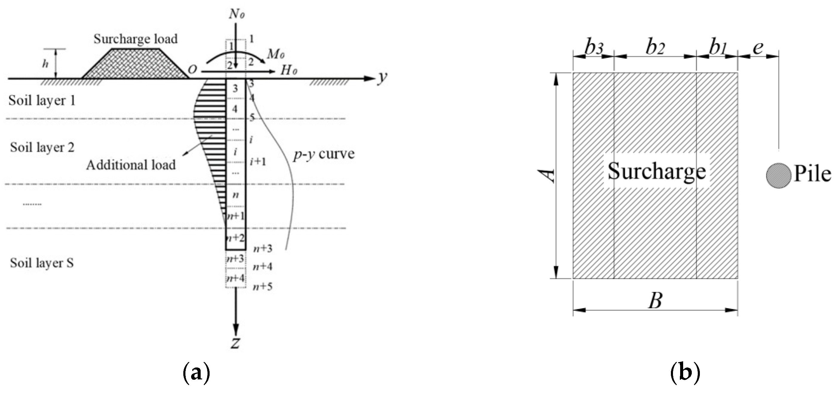
2.1. Calculation Model

For a single pile bearing an active load (pile-top vertical force  N 0 , pile-top horizontal force  H 0 , and pile-top bending moment  M 0 ), the pile top is assumed to be flush with the ground. The calculation model of an active–passive pile adjacent to a surcharge load is shown in Figure 1a. Assuming that the pile is composed of elastic material, the pile is considered to be a foundation beam placed vertically in the soil. The symbols of force and displacement are given as follows: the horizontal force and displacement are positive along the y-axis direction, and the positive bending moment indicates that the pile body at the side of the surcharge is under tension.
In Figure 1, A is the surcharge length (m), B is the total width of surcharge load (m),  b 1 b 2 b 3  are the surcharge widths (m), h is the surcharge height (m), e is the distance between the surcharge load and the pile (m), and L is the pile length (m).

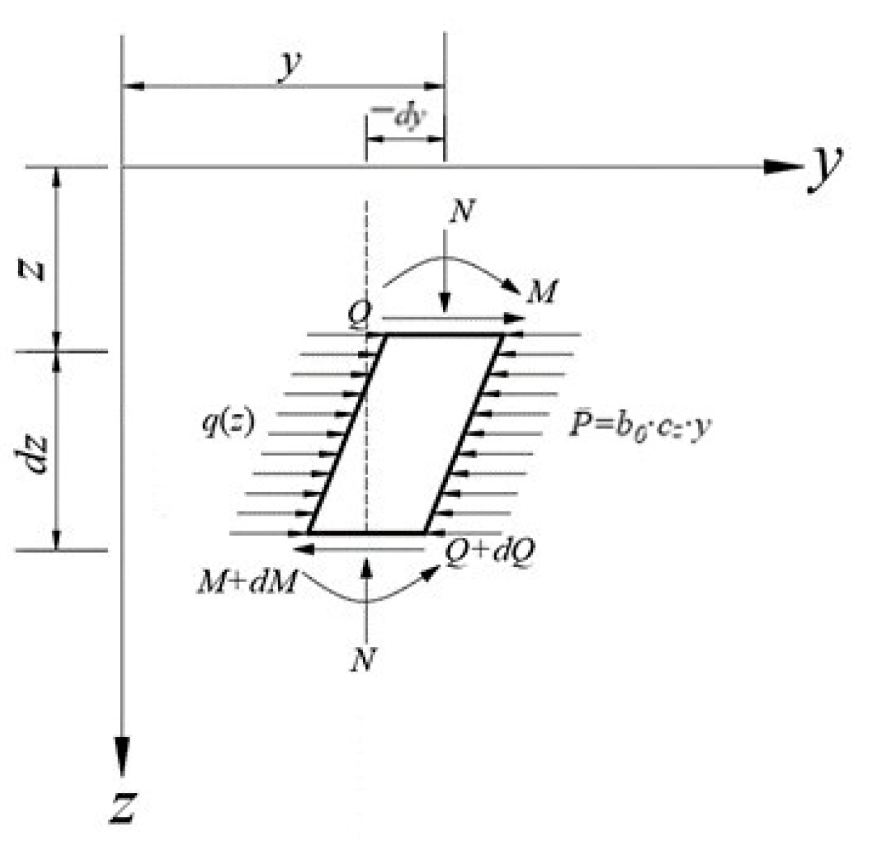
2.2. Establishment of The Flexural Differential Equation of the Pile

In order to study the internal force and deformation characteristics of an active–passive single pile adjacent to a surcharge load, we must first establish the pile’s flexural differential equation. This paper mainly analyzes the characteristics of the horizontal internal forces and the deformation of the pile shaft, so the axial force on the pile shaft is assumed to be constant during the calculations. Consider the pile element with length dz at depth z below the ground, as shown in Figure 2. Axial force (N), shear force (Q), and bending moment (M) act on the upper end of the element. The axial force (N), shear force (Q + dQ), and bending moment (M + dM) act on the lower end of the element. The pile side has soil resistance given by  P = b 0 c z y  and additional load  q z .
The force balance analysis of the pile body micro-element is carried out. Then the flexural differential equation of the pile can be given by
E I d 4 y d z 4 + N d 2 y d z 2 + b 0 c z y q z = 0
where EI is the bending stiffness of the pile (MPa·m4), N is the axial force acting on the pile (kN), cz is the horizontal resistance coefficient of foundation soil (MN/m4), cz = p/y, y is the pile horizontal displacement (m), z is the depth of the calculated point (m), q(z) is the additional line load concentration (kN/m). b0 is the calculated width of the pile (m), determined according to the relevant specifications [21].

2.3. Phase Description of the Additional Load Caused by an Adjacent Surcharge

With a change in factors such as an increase in the adjacent surcharge strength and the proximity of the surcharge distance, the soil around the pile gradually transits from the elastic to elastoplastic and plastic states. The calculation method for the pile additional side load corresponding to these different stages is given below.

2.3.1. Elastic State

The lateral pressure on the foundation caused by the surcharge is analyzed according to Figure 3. The surcharge is assumed to be a trapezoidally distributed load on a rectangular area, which can be thought of as a combination of the uniformly distributed loads and triangular distributed loads. According to the improved Boussinesq theory, the lateral additional load at point Q under the action of each load zone is calculated separately, and the total lateral additional load at this point can be obtained by the superposition. In the figure, p0 is the surcharge strength, and we assume that the surcharge width in the y-axis direction is a, the total width of the bottom of the surcharge load in the x-axis direction is B, the xoz plane is the symmetry plane in the y-axis direction, and the distance between the calculation point Q and the z-axis is e.
Horizontal additional pressure at point Q under a concentrated load micro-unit p0dxdy in the uniformly loaded rectangular area can be written as
d σ x z = 3 z π x e b 1 x e b 1 2 + y 2 + z 2 5 / 2 p 0 d x d y
In addition, the horizontal additional stress at point Q under uniform load on the rectangular area can be obtained by integration.
σ x 1 z = p 0 z π a e + b 1 e + b 1 2 + z 2 e + b 1 2 + a 2 + z 2 1 z arctan a e + b 1 z e + b 1 2 + a 2 + z 2 + 1 z arctan a e + b 1 + b 2 z e + b 1 + b 2 2 + a 2 + z 2 + a e b 1 b 2 e + b 1 + b 2 2 + z 2 e + b 1 + b 2 2 + a 2 + z 2
The horizontal additional stress at point Q under right and left rectangular area triangle loads can be written as
σ x 2 z = p 0 z π b 1 a b 1 e + b 1 e + b 1 2 + z 2 e + b 1 2 + a 2 + z 2 e z arctan a e + b 1 z e + b 1 2 + a 2 + z 2 + ln e + b 1 2 + z 2 e 2 + z 2 + e z arctan a e z e 2 + a 2 + z 2 + 2 ln a + e 2 + a 2 + z 2 a + e + b 1 2 + a 2 + z 2
σ x 3 ( z ) = p 0 z π b 1 a b 3 e + b 1 + b 2 e + b 1 + b 2 2 + z 2 e + b 1 + b 2 2 + a 2 + z 2 + ln e + b 1 + b 2 2 + z 2 ( e + B ) 2 + z 2 + 2 ln a + ( e + B ) 2 + a 2 + z 2 a + e + b 1 + b 2 2 + a 2 + z 2 e + B z arctan a e + b 1 + b 2 z e + b 1 + b 2 2 + a 2 + z 2 + e + B z arctan a ( e + B ) z ( a + B ) 2 + a 2 + z 2
The total horizontal additional stresses caused by the surcharge can be written as
σ x z = σ x 1 z + σ x 2 z + σ x 3 z
Finally, the passive line load set can be written as
q z = σ x z d

2.3.2. Elastoplastic State

Calculation Model and Formulas

When the soil around the pile is in an elastoplastic state, the earth pressure generated by the surcharge load can be calculated using an improved Ito theory:  θ 1 = π 8 + φ 4 θ 2 = π 4 φ 2 θ 3 = π 4 + φ 2 . Here, we assume that the wedge-shaped part of soil between piles ( A E B B E A ) reaches its ultimate strength under the influence of the soil lateral displacement and then enters the plastic state, while the rest of soil is still in the elastic state.
Force analysis of micro-units in area  A A E E  and area  E E B B  (the shaded area in Figure 4) is shown in Figure 5a,b, respectively. The static equilibrium differential equation in the x direction is given by
D 2 d σ x = 2 σ n tan φ + c d x
σ n + σ n tan φ + c N φ 1 / 2 σ x d D D d σ x = 0
where  σ n = σ x N φ + 2 c N φ 1 / 2 N φ = tan 2 π / 4 + φ / 2 d D = 2 d x N φ 1 / 2 , c is the soil-cohesive force, and φ is the soil internal friction angle.
These two differential equations can be solved separately to obtain
σ 1 x = C 1 exp 2 x N φ tan φ / D 2 c 2 N φ 1 / 2 tan φ + 1 N φ tan φ , 0 x D 1 D 2 2 tan π 8 + φ 4
and
σ 2 D = C 2 D N φ 1 / 2 tan φ + N φ 1 c 2 tan φ + 2 N φ 1 / 2 + N φ 1 / 2 N φ 1 / 2 tan φ + N φ 1 , D 2 x D 1
In the above two formulas,  σ 1 x  is the stress at any point x of zone  A A E E σ 2 D  is the stress at any point D of zone  E E B B , C1 and C2 are the undetermined integration constants, D1 is the centerline spacing between piles, and D2 is the net distance between the piles.
Taking the horizontal stress at plane  B B  as the initial boundary condition, and substituting  σ B B z = σ x z + K 0 γ z  into Equation (11) gives C2 so that  σ 2 D  can be written as
σ 2 D = 1 G 1 D D 1 G 1 σ B B z G 1 + c G 2 c G 2
C1 can be obtained according to the stress continuity condition ( σ 2 D | D = D 2 = σ 1 x | x = D 1 D 2 2 tan π 8 + φ 4 ) of the common boundary interface  E E  in zone  A A E E  and  E E B B , and thus  σ 1 x  can be written as
σ 1 x = exp 2 x N φ tan φ / D 2 N φ tan φ c 2 N φ 1 / 2 tan φ + 1 exp D 1 D 2 G 3 / D 2 + D 2 D 1 G 1 σ B B z G 1 + c G 2 c G 2 N φ tan φ G 1 exp D 1 D 2 G 3 / D 2 c 1 + 2 N φ 1 / 2 tan φ N φ tan φ
where  G 1 = N φ 1 / 2 tan φ + N φ 1 G 2 = 2 tan φ + 2 N φ 1 / 2 + N φ 1 / 2 , and  G 1 = N φ tan φ tan π / 8 + φ / 4 .

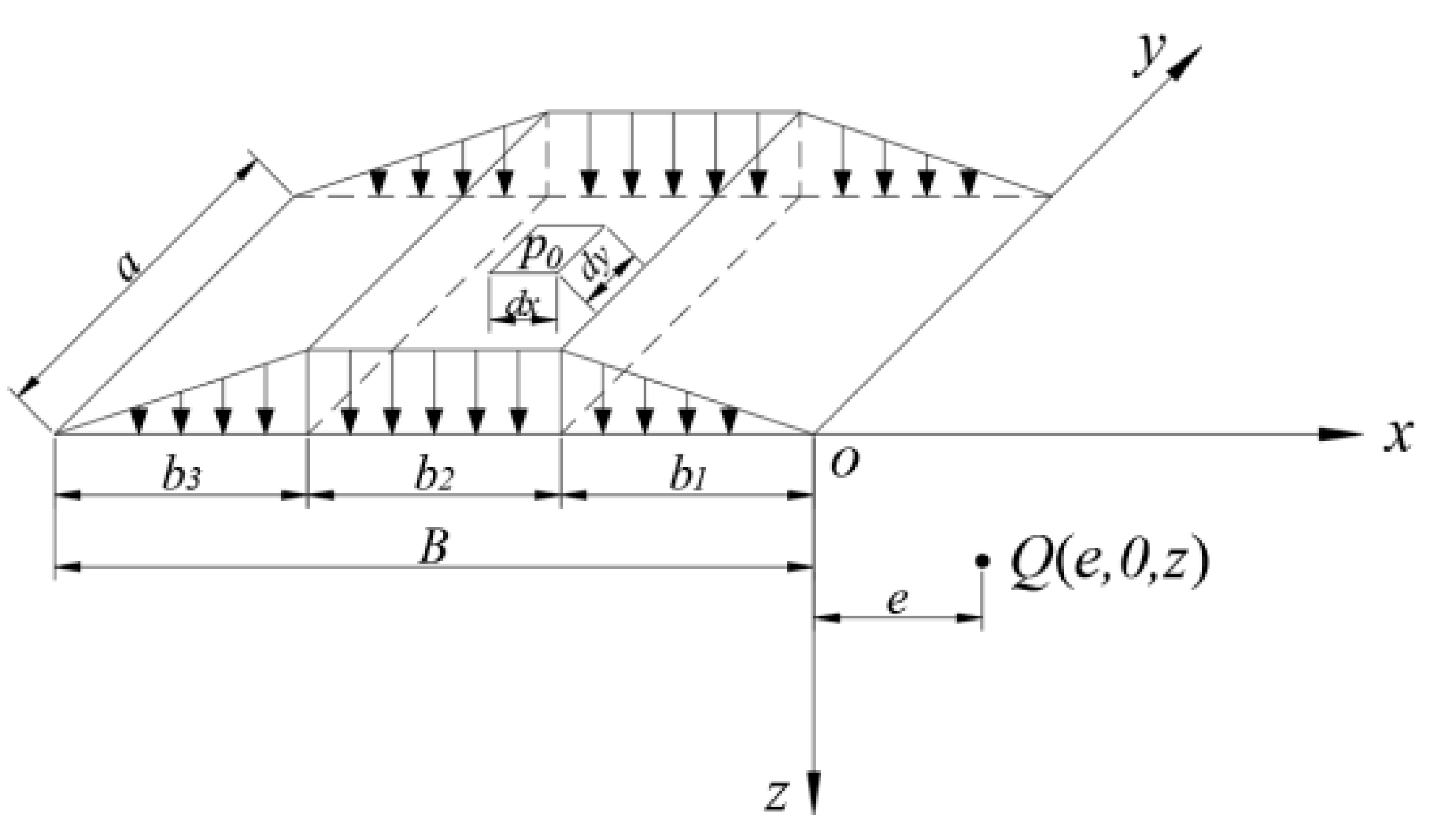
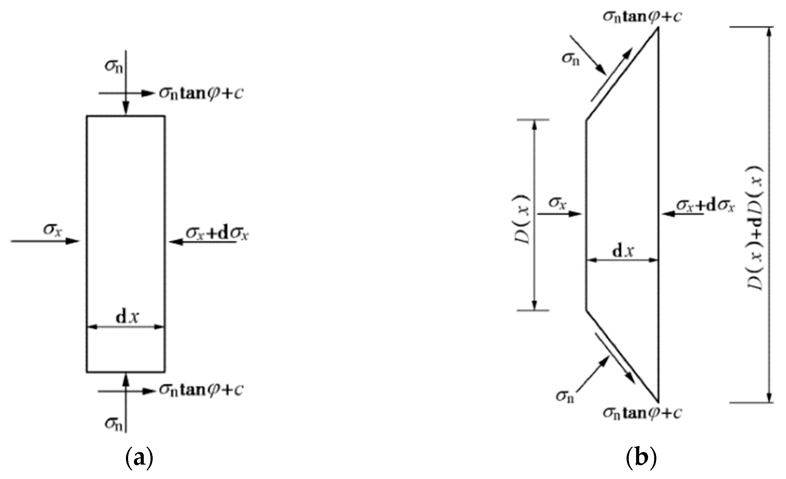
Calculation of the Additional Load on the Pile Side

We assumed that the earth pressure at rest  q 0 z = K 0 γ z  is the equilibrium stress of the soil mass between piles. When there is a horizontal stress at the AA′ surface  σ A A z > q 0 z , the plastic flow around the soil mass behind the pile occurs (which will be discussed later), and we now present the calculation method for  σ A A z q 0 z .
Step 1: calculate the total lateral pressure of surface BB′ under the influence of the surcharge.
σ B B z = σ x z + K 0 γ z
where  σ x z  is the additional stress calculated by Equation (6),  K 0  is the coefficient of earth pressure at rest, and  K 0 = 1 sin φ 0 , z is the depth of the calculated point.
Step 2: calculate the lateral pressure of surface  A A  under the influence of the surcharge.
σ A A z = 1 N φ tan φ c 1 + 2 N φ 1 / 2 tan φ exp D 1 D 2 G 3 / D 2 + D 2 D 1 G 1 σ B B z G 1 + c G 2 c G 2 N φ tan φ G 1 exp D 1 D 2 G 3 / D 2 c 1 + 2 N φ 1 / 2 tan φ N φ tan φ
Step 3: when  σ A A z K 0 γ z , find the new earth pressure equilibrium point. Substituting  σ 1 x = K 0 γ z  into Equation (13) gives  x = x l , and the next step is to determine the region where  x l  is located. If  x l  is in the region  A A E E , then the pile side passive line load concentration can be written as
q z = σ B B z D 1 σ 1 x | x = x l D 2
If  x l  is not in the region  A A E E σ 2 D = K 0 γ z  should be substituted into Equation (12), giving  D = D l , so that the pile side passive line load concentration can be written as
q z = σ B B z D 1 σ 2 D | D = D l D 2

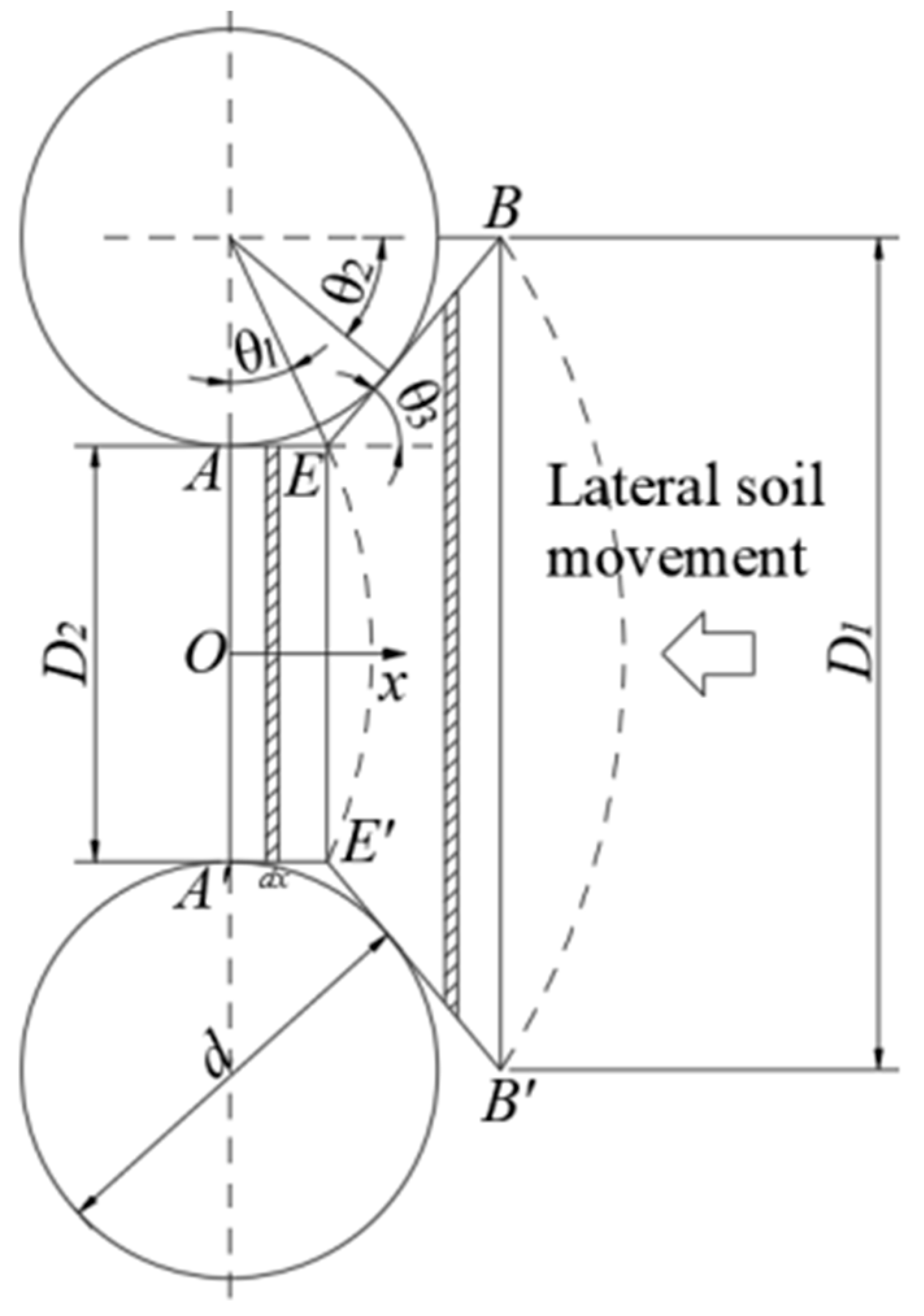
2.3.3. Plastic Flow State

As mentioned above, when  σ A A z > K 0 γ z , plastic flow occurs around the pile, and the passive load on the pile side is the ultimate load, which is calculated according to Equation (18) of Shen theory [8]:
q z = σ v + σ c 1 sin φ exp π 2 tan φ 4 tan 2 φ + 1 exp π tan φ 3 tan φ cos μ + 2 tan 2 φ 1 sin μ + 4 tan 2 φ + 1 1 sin φ sin μ + 3 tan φ sin μ 2 tan 2 φ 1 cos μ 4 tan 2 φ + 1 1 + sin φ cos μ d
where d is the pile diameter, and  μ = π / 4 + φ / 2 .

3. The Model’s Difference Equation and Its Solution

To solve the above model, the pile shaft is divided into n units vertically, each of length λ. For convenience, four virtual units are added at the top and bottom of the pile, and the unit and node numbers are shown in Figure 1. For any pile node i, the difference equation of node i can be obtained by substituting a one-dimensional central difference formula into Equation (1), according to the established pile deflection differential equation.
y i + 2 4 N λ 2 E I y i + 1 + 6 2 N λ 2 E I + b 0 c z i λ 4 E I y i 4 N λ 2 E I y i 1 + y i 2 q i λ 4 d E I = 0
Substituting  4 N λ 2 E I = k b 0 c z i λ 4 E I = A i  and  λ 4 d E I = G  into Equation (19), Equation (19) can be written as
y i + 2 k y i + 1 + 2 k 2 + A i y i k y i 1 + y i 2 G q i = 0
Corresponding rotation ( θ i ), bending moment ( M i ), and shear force ( Q i ) can be obtained as
θ i = 1 2 λ y i + 1 y i 1
M i = E I λ 2 y i + 1 2 y i + y i 1
Q i = d M d z + N d y d z = E I 2 λ 3 y i + 2 2 y i + 1 + 2 y i 1 y i 2 + N 2 λ y i + 1 y i 1
An equilibrium equation such as Equation (19) can be obtained for any pile shaft node i. There are n + 1 equations. To solve the system, four supplementary equations need to be determined from the boundary conditions. Two equations can be derived using the known active load of the pile top:
M 3 = E I λ 2 y 4 2 y 3 + y 2 = M 0
Q 3 = E I 2 λ 3 y 5 2 y 4 + 2 y 2 y 1 + N 2 λ y 4 y 2 = H 0
and the other two can be derived according to the boundary conditions for the pile bottom.
When the pile bottom is not embedded in the rock stratum, it can be regarded as free. That is, the shear force at node n + 3 is 0. When the pile bottom is supported in the soil layer and  α l 2.5  or the pile end is supported in the rock stratum and  α l 3.5 , the section deformation of the pile bottom is very small. Thus, the bending moment at the pile bottom can treated as 0:
M n + 3 = E I λ 2 y n + 4 2 y n + 3 + y n + 2 = 0
Q n + 3 = E I 2 λ 3 y n + 5 2 y n + 4 + 2 y n + 2 y n + 1 + N 2 λ y n + 4 y n + 2 = 0
When the pile end is embedded in the rock stratum, it is regarded as fixed, and in this case, the section angle and displacement at node n + 3 are 0:
θ n + 3 = 1 2 λ y n + 4 y n + 2 = 0
y n + 3 = 0
Here, the equations are formed by combining the different pile bottom boundary conditions, pile-top load conditions, and pile node difference equations. After solving this system of equations, all node displacements  y i  can be obtained successively from  y 0 . Then, the rotation, bending moment, and shear force of each node of the pile can be obtained by Equation (21) through Equation (23). In fact, since the horizontal displacement ( y i ) of pile at point i is unknown,  c z i  cannot be determined from the py curve. Therefore, the iterative method (as below) should be used to calculate the pile displacement and internal force. First, assume the initial value of  c z i , and obtain  y i  (the horizontal displacement of each node of pile) by using the finite difference method successively. The corresponding  p i  can then be obtained from the py curve, and  c z i  is then given by  c z i = p i / y i y i  is recalculated using the finite difference method until it converges.
The analytical solutions’ differential equations with initial and boundary value conditions can often not be obtained through theoretical derivation. An effective way is to obtain the approximate solutions with a certain numerical accuracy by using numerical methods, including finite difference method, numerical integration method, Bezier Method, inverse differential quadrature method, etc. For example, Khalid [22] proposed a new two-dimensional inverse differential quadrature method to approximate the solution of high-order differential equations. Kabir [23] extended a robust Bezier-based multi-step method to accurately solve the governing fourth order complex partial differential equation in linear elastic fracture mechanics problems.

4. Validation of the Calculation Method

Due to the lack of active–passive single pile test data, the active pile case and the passive pile case are now used to evaluate the correctness of the above active and passive single pile calculation methods.

4.1. Analysis of an Active Pile Based on a Typical p–y Curve

A case of active pile in Zhenjiang [24] was selected in order to evaluate the correctness of the methods and procedures in this paper for active pile analysis. The site test pile in this case is a steel pipe with a buried depth of 45 m and a diameter of 1.2 m. The pile stiffness is EI = 2.88 × 10⁶ kN·m2, and the average undrained shear strength of the soil measured by static triaxial test is 54 kPa. The horizontal load acts on the pile top, and the action position of the horizontal load is 7.9 m above the ground. Finally, the horizontal displacement of the pile on the ground and the maximum bending moment of the pile were obtained when the horizontal load was 20 kN, 50 kN, 100 kN, 150 kN, 200 kN, 250 kN, and 300 kN. In this paper, the pile top in the calculation model is assumed to be flush with the ground, so according to the principle of force equivalence, the test load is equivalent to the horizontal load and bending moment at the ground.
Three typical py curves (Zhang [25], Wang [26], and Matlock [27]) applicable to soft clay in Table 1 were selected to describe the relationship between the lateral soil resistance and the horizontal displacement of the pile. The relevant parameters of the py curve are taken from the literature. DIAPP was used to calculate the horizontal displacement of the pile top and the maximum bending moment of the pile body under different loads, and the calculated results were then used to compare to the field measured data, as shown in Figure 6a,b.
In the table,  y 50  is the corresponding lateral deformation of the pile body when the soil around the pile reached half of the ultimate soil resistance (mm),  p u  is the ultimate soil resistance at the pile side (kPa),  F s  is the reduction coefficient closely related to soil properties and load forms, and a and b were determined by triaxial test.
Figure 6 shows that under the same load, the ranking of the horizontal displacement of the pile top and the maximum bending moment of the pile body calculated using three py curve models is Zhang model > Wang model > Matlock model. The pile-top displacement calculated using the Zhang model is larger than the test results, while the results obtained using the Wang model or Matlock model are smaller than the test results. The maximum bending moment of the pile calculated using the three models is slightly larger than the test values. The variation trend of the above calculated values with the load based on the three models is consistent with the field measured results, and they all increase nonlinearly with the horizontal load, which supports the correctness of the method in this paper.
Since the horizontal displacements of the pile top calculated by the py curve model of Wang and Matlock are slightly less than the measured value, we chose the Zhang model for subsequent analysis.

4.2. Passive Pile Analysis Based on Staged Descriptions of Additional Loads

A passive pile test in Ningbo [6] was selected to judge the correctness of the method and program in this paper further. Table 2 describes the soil layer distribution and calculation parameters of the test site. The site test pile is a cast-in-place bored pile with a length of 45 m, a diameter of 1.0 m, and a pile spacing of 3.0 m. The stiffness of this reinforced concrete pile is  E I = 1.65 × 10 6   kN m 2 , and the surcharge strength is 70.0 kPa. In this case the load is formed by filling the soil in a rectangular area (surcharge length (A = 25.0 m), surcharge width (B = 10.0 m)). Finally, the surcharge distances (e in Figure 1b) are 15 m (working condition 1) and 10 m (working condition 2).
The test results for the pile displacement and bending moment under the two working conditions were compared with our calculation results, as shown in Figure 7 and Figure 8. In the figures, the positive displacement indicates that the pile deviates away from the surcharge load, and the positive bending moment means that the pile is strained on the side of the surcharge load. According to the measured results, the maximum horizontal displacement occurs at the top of the pile under both the working conditions, and the pile displacement gradually decreases along the depth direction. If the horizontal displacement of the pile is greater than or equal to 0.2 mm, the horizontal displacement of the pile in condition 1 and condition 2 occurs in the range of about 22 m (2.2B) and 28 m (2.8B) below the ground, respectively. This is obviously greater than the pile displacement depth 9.4 m calculated by elastic analysis when the pile is in an active pile condition (calculated by the “m” method, at  α z = 4.0  [15]), and it increases as the distance between the pile and surcharge load decreases.
From the pile top to pile bottom, the pile-bending moment changes from a negative moment of load side compression to a positive moment of load side tension under both conditions. The extreme point of the negative bending moment is located at a depth of 6.5 m, which is close to the interface between the mixed fill soil and silt layer (depth of 4.8 m), and the extreme point of the positive bending moment is located at a depth of 14 m, which is close to the interface between the silt layer and silty clay layer (depth of 13.1 m). This experimental phenomenon is also consistent with the conclusion obtained by Stewart [28] from a model test where the maximum pile-bending moment occurred near the pile top or near the interface between soft and hard soil.
Figure 7 shows the comparison between the calculation and measured results under working condition 1. Here, we can see that the pile displacement at the ground does not exceed 6.0 mm (the passive load was calculated using the improved Boussinesq theory), and the calculated results agree with the experimental results. The calculated value of pile-top displacement is 21.61 mm, and the corresponding test value is 4.01 mm. The calculated maximum bending moment of the pile shaft is 59.45 kN, and the corresponding test value is 107.48 kN. The difference between the calculated pile-top displacement and the measured value is only 3.1%, and the relative error of the pile maximum bending moment is 44.6%.
Figure 8 shows that the pile displacement and pile-bending moment calculated under working condition 2 are basically consistent with the measured results. The calculated maximum bending moment of the pile shaft is 297.09 kN, which is 3.97 kN greater than the test value. The calculated value of pile-top displacement is 21.61 mm, which is 1.71 mm larger than the test value. The relative error between the calculated pile-top displacement and measured result is only 6.7%, and the relative error between the maximum pile-bending moment and measured result is only 0.5%. Figure 9 shows the additional load caused by the same surcharge when the surcharge distance (e) and the surcharge width (B) are different. The black curve in Figure 9a corresponds to working condition 2. Our calculation results show that the horizontal displacement of the pile within 10.5 m below the ground is greater than 6 mm, that the soil around the pile within 4 m of the buried depth is in the plastic flow state, and that the soil around the pile within the buried depth of 4 m to 10.5 m is in an elastoplastic state. The displacement of the pile body with a buried depth greater than 10.5 m is less than 6 mm, and the soil around the pile side is in the elastic state.
Figure 9 shows that when other factors are the same, as the surcharge distan€(e) changes from 5 m (0.5B) to 15 m (1.5B), the additional load gradually decreases, and the maximum additional load decreases from 99.54 kN/m to 20.40 kN/m, about 79.5%. In addition, the position of the maximum additional load gradually moves upward from a depth of about 10.5 m (0.23 L) to a depth of about 5.0 m (0.11 L). When the surcharge width (B) changes from 5 m to 15 m, the maximum additional load increases from 21.16 kN/m to 71.52 kN/m, a factor of approximately 2.4 times. The position of the maximum additional load gradually moves down with the increase in the stacking width, and its position moves down from a depth of about 7 m (0.16 L) to a depth of about 8.5 m (0.19 L). We thus consider our method to be highly applicable for calculating the passive load caused by the adjacent surcharges in nonlinear settings.

5. Conclusions

In this paper, the differential equation for the pile deflection was established for an active–passive single pile whose top is flush with the ground. Based on a staged description of the additional load caused by an adjacent surcharge, the analysis of the internal forces and deformation of the active–passive single pile using a typical py curve to describe the relationship between the lateral soil resistance and the horizontal displacement of the pile was realized. The obtained results and mechanical analysis lead us to the following conclusions, enumerated below.
(1)
For a given surcharge condition, the soil around the pile at different buried depths may be in a plastic flow, elastoplastic, or elastic state. The staged description of the additional load set against these states is helpful for the accurate calculation and analysis of the pile foundation.
(2)
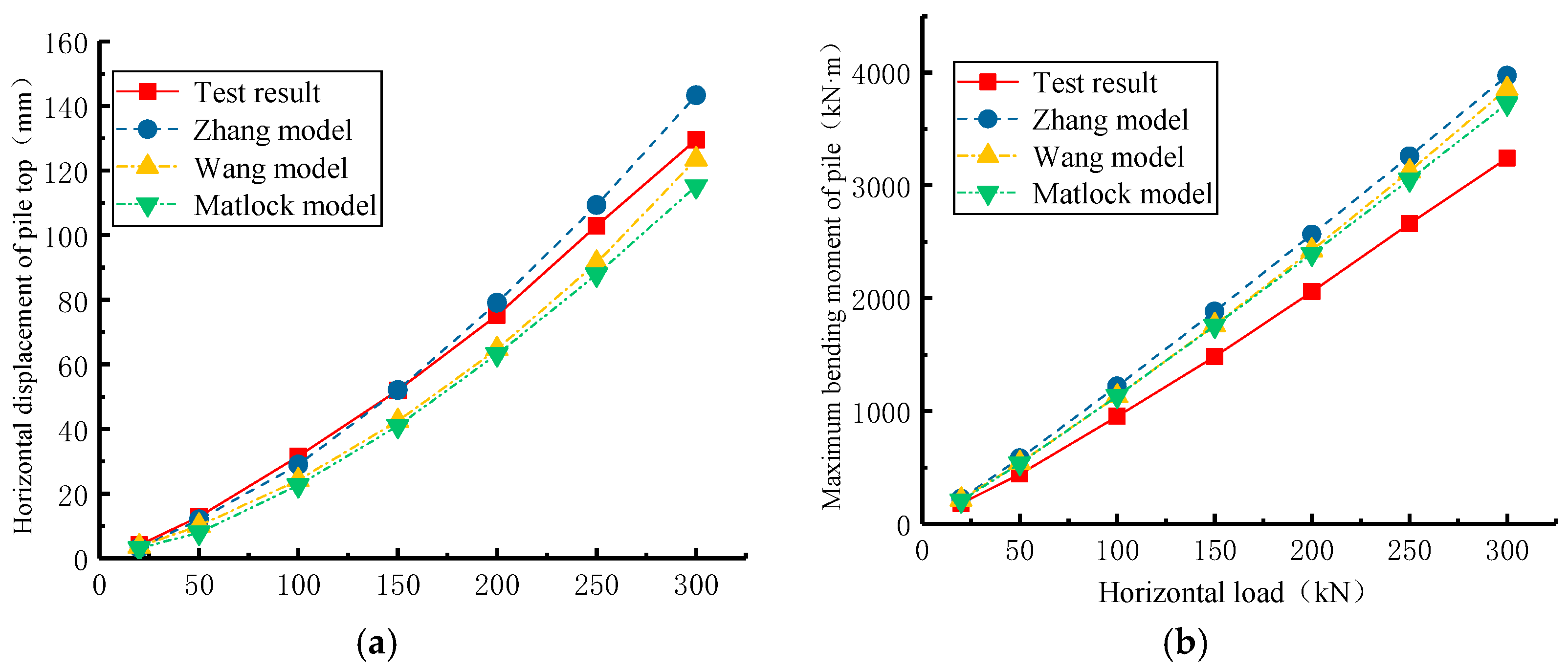
The order of horizontal displacement of pile top and maximum bending moment of pile shaft calculated from three typical py curves applicable to soft clay can be arranged as follows: Zhang model > Wang model > Matlock model. Additionally, the horizontal displacement of the pile top and the maximum bending of the pile increase nonlinearly with the horizontal load on the pile top. The variation trend and values were also consistent with the measured results. The calculated value of Zhang’s model was the closest to the measured results.
(3)
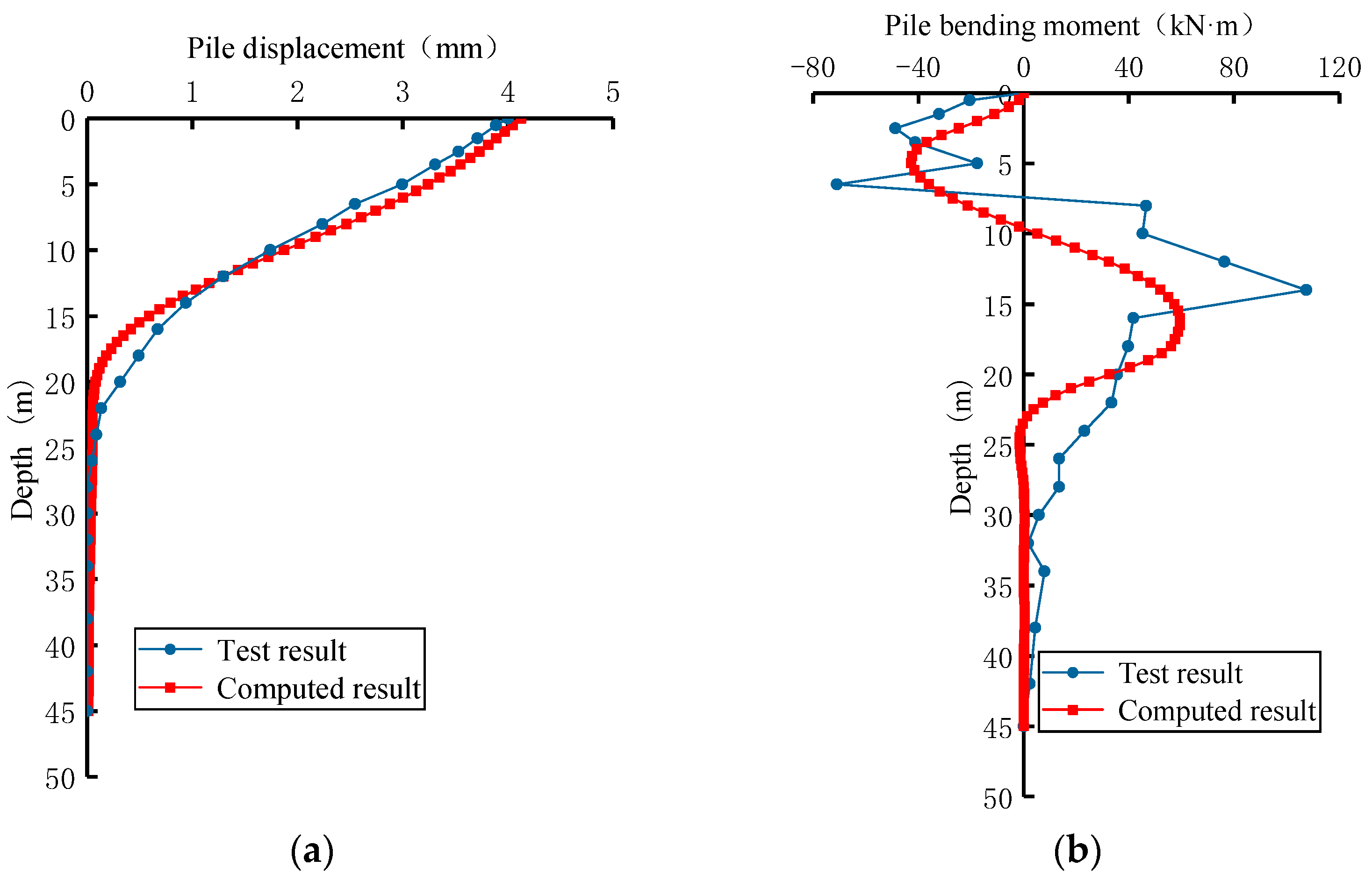
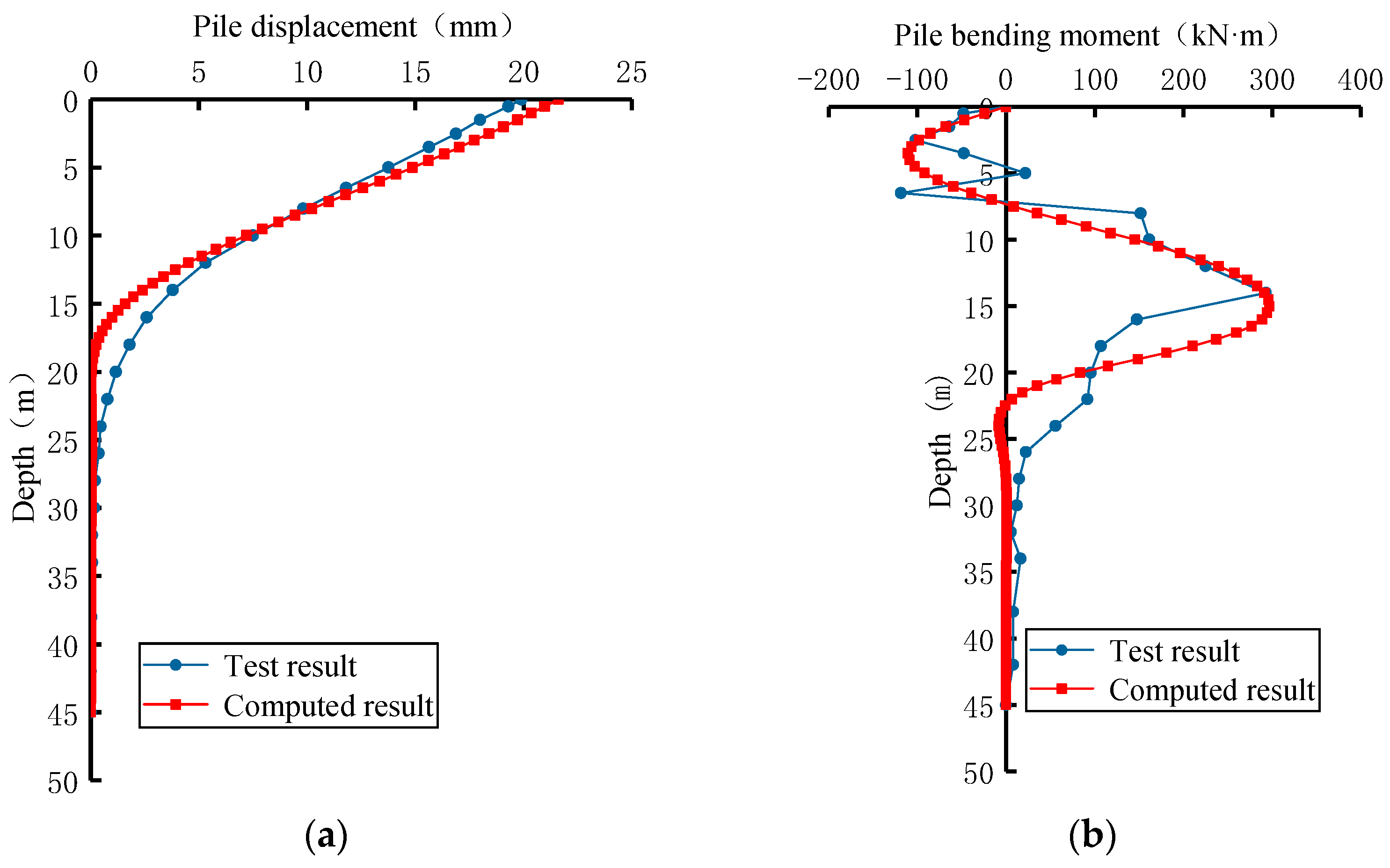
The displacement of the pile caused by the adjacent surcharge decreases gradually along the depth direction. The depth range of the horizontal displacement of the pile under a passive load is significantly greater than that under an active load. The extreme value of the pile shaft bending moment appears near the interface between the soft and hard soil layers.
(4)
The method in this paper reflects the nonlinear characteristics of pile–soil interaction with a typical py curve. It can thus be applied to the mechanical response analysis of active–passive single piles adjacent to heaped loads.
Because of the lack of test cases of an active–passive pile, this paper used the test cases of pure active pile and pure passive pile to verify the calculation method. In addition, this study failed to analyze the situation of multi-row piles, which is also a problem that we need to study further.

Author Contributions

Writing—review and editing, L.W., Q.H. and C.Z.; Supervision, L.W.; Software, K.Z. and C.Z.; Writing—original draft preparation, K.Z.; Data curation, Q.H. and K.Z. All authors have read and agreed to the published version of the manuscript.

Funding

This research work was financially supported by the National Natural Science Foundation of China (Grant No. 51878671).

Institutional Review Board Statement

Not applicable.

Informed Consent Statement

Not applicable.

Data Availability Statement

Not applicable.

Conflicts of Interest

The authors declare no conflict of interest.

References

  1. Ellis, E.A.; Springman, S.M. Modelling of soil-structure interaction for a piled bridge abutment in plane strain FEM analyses. Comput. Geotech. 2001, 28, 79–98. [Google Scholar] [CrossRef]
  2. Li, H.; Liu, S.; Yan, X.; Gu, W.; Tong, L. Effect of loading sequence on lateral soil-pile interaction due to excavation. Comput. Geotech. 2021, 134, 104134. [Google Scholar] [CrossRef]
  3. Springman, S.M. Lateral Loading on Piles Due to Simulated Embankment Construction. Ph.D. Thesis, University of Cambridge, Cambridge, UK, 1989. [Google Scholar]
  4. Liu, H.L.; Jian, C.; An, D. Use of large-diameter, cast-insitu concrete pipe piles for embankment over soft clay. Can. Geotech. J. 2009, 46, 915–927. [Google Scholar] [CrossRef] [Green Version]
  5. Yuan, B.; Chen, M.; Chen, W.; Luo, Q.; Li, H. Effect of pile-soil relative stiffness on deformation characteristics of the laterally loaded pile. Adv. Mater. Sci. Eng. 2022, 2022, 1–13. [Google Scholar] [CrossRef]
  6. Li, H.; Wei, L.; Feng, S.; Chen, Z. Behavior of piles subjected to surcharge loading in deep soft soils: Field tests. Geotech. Geol. Eng. 2019, 37, 4019–4029. [Google Scholar] [CrossRef]
  7. Gu, M.; Cai, X.; Fu, Q.; Li, H.; Wang, X.; Mao, B. Numerical Analysis of Passive Piles under Surcharge Load in Extensively Deep Soft Soil. Buildings 2022, 12, 1988. [Google Scholar] [CrossRef]
  8. Yang, M.; Shangguan, S.; Li, W.; Zhu, B. Numerical study of consolidation effect on the response of passive piles adjacent to surcharge load. Int. J. Geomech. 2017, 17, 04017093. [Google Scholar] [CrossRef]
  9. Li, S.; Wei, L.; Feng, S.; He, Q.; Zhang, K. Time-dependent interactions between passive piles and soft soils based on the extended Koppejan model. Rock Soil Mech. 2022, 43, 2602–2614. [Google Scholar]
  10. Mingxing, Z. Research on Bearing Mechanism of Passive Pile under Combined Loads. Ph.D. Thesis, Southeast University, Nanjing, China, 2016. [Google Scholar]
  11. Ito, T.; Matsui, T. Methods to estimate lateral force acting on stabilizing piles. Soils Found. 1977, 15, 43–59. [Google Scholar] [CrossRef] [Green Version]
  12. Ito, T.; Matsui, T.; Hong, W.P. Design method for the stability analysis of the slope with landing pier. J. Apanese Soc. Soil Mech. Found. Eng. 1979, 19, 43–57. [Google Scholar] [CrossRef] [Green Version]
  13. Hao, Z.; Minglei, S.; Yuancheng, G.; Weizheng, L. Lateral mechanical behaviors of structural piles adjacent to imbalanced surcharge loads. Chin. J. Geotech. Eng. 2016, 38, 2226–2236. [Google Scholar]
  14. Zhujiang, S. Ultimate lateral resistance and limit design of stabilizing pile. Chin. J. Geotech. Eng. 1992, 14, 51–56. [Google Scholar]
  15. Li, Z.; Liang, Z. Calculation model and numerical analysis of passive piles subjected to adjacent surcharge loads. Chin. J. Geotech. Eng. 2010, 32, 128–134. [Google Scholar]
  16. Zhao, M.H.; Yin, P.B.; Yang, M.H.; Yong, L. Analysis of influence factors and mechanical characteristics of bridge piles in high and steep slopes. J. Cent. South Univ. (Sci. Technol.) 2012, 43, 2733–2739. [Google Scholar]
  17. Liang, F.; Yu, F.; Han, J. A simplified analysis method for an axially loaded single pile subjected to lateral soil movement. J. Tongji Univ. (Nat. Sci.) 2011, 39, 807–813. [Google Scholar]
  18. Wei, L.; Wang, J.; Zhai, S.; He, Q. Analysis of internal force and displacement of axial transverse composite loaded pile in layered soft soil foundation. J. Railw. Sci. Eng. 2021, 18, 2907–2915. [Google Scholar]
  19. Minghui, Y.; Yuhui, W.; Chaobo, F. Calculation method of horizontal loaded piles near slope based on passive wedge model. J. Railw. Sci. Eng. 2019, 16, 2951–2959. [Google Scholar]
  20. Zhang, H.; Shi, M.; Guo, Y. Semianalytical solutions for abutment piles under combined active and passive loading. Int. J. Geomech. 2020, 20, 04020171. [Google Scholar] [CrossRef]
  21. National Railway Administration of the People’s Republic of China. Code For Design On Subsoil and Foundation Of Railway Bridge And Culvert: TB 10093-2017; China Railway Press: Beijing, China, 2017. [Google Scholar]
  22. Khalid, H.M.; Ojo, S.O.; Weaver, P.M. Inverse differential quadrature method for structural analysis of composite plates. Comput. Struct. 2022, 263, 106745. [Google Scholar] [CrossRef]
  23. Kabir, H.; Aghdam, M.M. A generalized 2D Bézier-based solution for stress analysis of notched epoxy resin plates reinforced with graphene nanoplatelets. Thin-Walled Struct. 2021, 169, 108484. [Google Scholar] [CrossRef]
  24. Ziai, L. Study on modulus of subgrade reaction for lateral loaded piles in multiple layered foundation. Chin. J. Geotech. Eng. 1988, 10, 48–56. [Google Scholar]
  25. Lianyang, Z.; Zhuchang, C. Method for calculating p-y curve of cohesive soil. Ocean. Eng. 1992, 4, 50–58. [Google Scholar]
  26. Huichu, W.; Dongqing, W. A new unified method for p-y curve of lateral static piles in clay. J. Hohai Univ. (Nat. Sci. Ed.) 1991, 1, 9–17. [Google Scholar]
  27. Matlock, H. Correlation for design of laterally loaded piles in soft clay. In Offshore Technology in Civil Engineering; ASCE: Reston, VA, USA, 1970; pp. 77–94. [Google Scholar]
  28. Stewart, D.P.; Ewell, R.; Randolph, M.F. Design of piled bridge abutments on soft clay for loading from lateral soil movements. Géotechnique 1994, 44, 277–296. [Google Scholar] [CrossRef]
Figure 1. Calculation model diagram of a single pile using our coordinate system. (a) Elevation; (b) plane.
Applsci 13 04196 g001
Figure 2. Schematic diagram for the stress analysis of a foundation pile.
Applsci 13 04196 g002
Figure 3. Diagram of the surcharge load.
Applsci 13 04196 g003
Figure 4. Calculation model using an improved Ito theory.
Applsci 13 04196 g004
Figure 5. Stress analysis of a micro-unit in the plastic zone. (a) Zone  A A E E ; (b) zone  E E B B .
Applsci 13 04196 g005
Figure 6. Test and calculation results of different py curves. (a) Horizontal displacement of the pile top; (b) maximum bending moment of the pile shaft.
Applsci 13 04196 g006
Figure 7. The calculated and measured values for working condition 1 (e = 15 m). (a) Pile displacement; (b) pile-bending moment.
Applsci 13 04196 g007
Figure 8. The calculated and measured values in working condition 2 (e = 10 m). (a) Pile displacement; (b) pile-bending moment.
Applsci 13 04196 g008
Figure 9. The additional load acting on the pile shaft (surcharge strength is 70 kPa; surcharge length (A) is 25 m). (a) Additional load changing with depth with different surcharge distances (surcharge width (B) is 10 m). (b) Additional load changing with depth with different surcharge widths (surcharge distance € is 10 m).
Applsci 13 04196 g009
Table 1. py curve expression.
Computational Modelpy Curve Expression
Zhang Model [17] p = 0.5 p u y / y 50 1 / 3      y 8 y 50 F s + 1 F s x / x r p u y > 8 y 50 , z z r s p u            y > 8 y 50 , z > z r s
Wang Model [18] p = y / y 50 a + b y / y 50 p u   y β y 50 p u     y > β y 50
Matlock model [19] p = 0.5 p u y / y 50 1 / 3   y 8 y 50 p u   y > 8 y 50
Table 2. Calculation parameters of the soil layers.
Soil LayerSoil Thickness (m)Density
(kg/m3)
Modulus of Compression (MPa)Cohesion
(kPa)
Internal Friction Angle (°)
Miscellaneous fill4.81800-511.5
Mud8.316422.0910.510.2
Silty clay with silty soil4.818774.3112.212.8
Muddy silty clay12.617333.2411.911.2
Silty clay12.717424.6315.312.3
Silty clay1.917743.7724.111.3
Disclaimer/Publisher’s Note: The statements, opinions and data contained in all publications are solely those of the individual author(s) and contributor(s) and not of MDPI and/or the editor(s). MDPI and/or the editor(s) disclaim responsibility for any injury to people or property resulting from any ideas, methods, instructions or products referred to in the content.

