Exploration of Vehicle Target Detection Method Based on Lightweight YOLOv5 Fusion Background Modeling

Abstract

Due to the explosive increase per capita in vehicle ownership in China brought about by the continuous development of the economy and society, many negative impacts have arisen, making it necessary to establish the smart city system that has rapidly developing vehicle detection technology as its data acquisition system. This paper proposes a lightweight detection model based on an improved version of YOLOv5 to address the problem of missed and false detections caused by occlusion during rush hour vehicle detection in surveillance videos. The proposed model replaces the BottleneckCSP structure with the Ghostnet structure and prunes the network model to speed up inference. Additionally, the Coordinate Attention Mechanism is introduced to enhance the network’s feature extraction and improve its detection and recognition ability. Distance-IoU Non-Maximum Suppression replaces Non-Maximum Suppression to address the issue of false detection and omission when detecting congested targets. Lastly, the combination of the five-frame differential method with VIBE and MD-SILBP operators is used to enhance the model’s feature extraction capabilities for vehicle contours. The experimental results show that the proposed model outperforms the original model in terms of the number of parameters, inference ability, and accuracy when applied to both the expanded UA-DETRAC and a self-built dataset. Thus, this method has significant industrial value in intelligent traffic systems and can effectively improve vehicle detection indicators in traffic monitoring scenarios.

1. Introduction

In recent years, the increasing car ownership in China has led to traffic congestion, long commute times, traffic accidents, and environmental problems. To address these issues, authorities have resorted to infrastructure construction methods such as building viaducts and widening roads. However, these solutions are resource-intensive and do not tackle the root cause of the problem. Therefore, several developing countries are focusing on developing technologies related to intelligent transportation systems (ITS) to improve traffic management effectiveness [1]. Vehicle detection is an essential auxiliary system of ITS. With the evolution of computer vision, vehicle detection technology has become a topic of significant interest among scholars.

Vehicle detection, being the primary task of intelligent transportation systems, plays a crucial role in determining the efficacy of the entire intelligent system. Motion-based vehicle detection methods can be categorized into three types: optical flow [2], frame difference [3], and background difference [4]. The optical flow method is based on optical flow fields, which are first extracted from the image and combined with image feature information for target detection. However, this method is computationally intensive and cannot achieve real-time detection. The frame difference method detects motion regions by subtracting two adjacent frames in a video sequence, which generates a large number of voids when traffic video speeds are high. The background difference method involves building a background model and comparing it with the video sequence frame by frame. If the video image frame is the same as the exact position of the built background model, it is identified as the background and updated to the background model. However, this method is less robust, more sensitive to illumination and noise, and more time-consuming to reconstruct than the background model. Wang’s proposed background modeling algorithm employs inter-frame difference and the Gaussian mixture model while also utilizing the Harris corner detection method to accurately detect moving objects. Although the algorithm exhibits impressive detection accuracy and real-time performance, its practical application still requires further development [5]. Yin introduced a method for enhancing vehicle camera monitoring systems which relies on fast background modeling and adaptive moving target detection. The core idea of this method is to constantly update the background model to enable for the efficient detection of moving targets within real-time video streams. Although the approach showcases promising results, its detection outputs might not suffice to support follow-up research. Further research and refinement are necessary to enhance its detection capabilities and maximize its potential in vehicle monitoring applications [6].

With the continuous advancement of machine learning and GPU parallel processing capability, deep learning-based target detection has become a popular research topic. It can be classified into region candidate-based target detection and regression-based target detection. Region candidate-based target detection, also known as the Two-Stage target detection algorithm, generates candidate regions and classifies them based on regions, with the R-CNN series [7,8,9] being a classical algorithm in this category. Regression-based target detection algorithms, also known as One-Stage target detection algorithms, can simultaneously identify targets and determine their location. Examples of representative algorithms in this category include SSD [10] and YOLO series [11,12,13,14,15]. The original YOLOv5 model suffers from generating redundant feature information during feature extraction in vehicle detection, leading to a large model size and slow inference. To address this, lightweight networks such as SqueezeNet, MobileNet, ShuffleNet, and Xception have been used to prune operations by compressing the number of feature maps or reducing the number of parameters through depth-wise convolution and improved series. However, such methods can effectively reduce the number of parameters but result in a loss in detection accuracy. Despite meeting lightweight requirements, lightweight networks such as the MobileNet series, YOLOv3-tiny, and YOLOv4-tiny series are unable to maintain model detection accuracy. The YOLOv5-s model can meet the requirements of needing to be lightweight and have good performance in the COCO dataset. Wang et al. [16] proposed YOLOv4, which introduced depth-separable convolution and the CBAM attention mechanism, improving the detection accuracy while reducing the model computation. Li et al. [17] proposed an improved YOLOv5 combined with the DeepSort traffic statistical computation method and incorporating the CBAM attention mechanism, which further improves the detection accuracy. However, the redundant feature map information is not processed, and the model size and inference speed are too slow for deployment on monitoring terminals. Lu et al. [18] proposed a novel approach for real-time multiple-vehicle detection and tracking from a moving platform. The method integrates vehicle detection with vehicle tracking and utilizes convolutional neural networks (CNNs) and deep reinforcement learning for improved accuracy and robustness. Meng et al. [19] proposed a tracking-by-detection approach for vehicle tracking in unmanned aerial vehicle (UAV) videos. The proposed method combines deep learning techniques with motion cues for detecting and tracking vehicles in challenging aerial scenarios.

To improve the detection performance of the model and speed up inference, this paper proposes an improved YOLOv5 model for vehicle object detection in traffic monitoring. The proposed method has the following contributions:

(1)

There are numerous superfluous and redundant neurons within the bottleneck feature extraction network. Replacing the CSP structure with the GhostNet structure can significantly decrease both model parameters and computational resources. Furthermore, substituting the conventional parallel three-layer maximum pooling operation with the SPPF structure and serial three-layer maximum pooling can enhance the model’s reasoning capabilities further.

(2)

In traffic monitoring scenarios, the improved YOLOv5 model incorporates CA attention mechanisms in the backbone, neck, and head to enhance the extraction of essential features and suppress the extraction of general features, thereby improving detection accuracy. To tackle vehicle occlusion, DIoU-NMS is employed to accelerate the regression of a suitable target box for detecting vehicles.

(3)

To improve the detection accuracy by highlighting the vehicle contour feature information, a method is proposed in this paper. Firstly, the five-frame difference method of the perceptual hash image search algorithm is used to obtain a complete background model, which can avoid the ghost phenomenon. Then, the image frames are transformed to the YCrCb color space to roughly determine the shadows. After that, the MD-SILBP operator is used for accurate shadow recognition and rejection, which helps obtain the complete vehicle foreground for feature recognition and extraction.

2. Network Model

2.1. YOLOv5 Model

YOLOv5 is the latest version of the YOLO series, which uses a new design approach—implementing a lighter model and employing new design methods to ensure detection accuracy. The YOLOv5 model, based on the PyTorch framework, is extremely lightweight, reducing the model size by nearly 90% compared to YOLOv4. At the same time, YOLOv5 has a faster detection speed while maintaining accuracy, making it more advantageous in practical applications. YOLOv5 includes four versions: S, M, L, and X, with the S version having the fastest detection speed. The network layer number of the other versions increases in order. In this chapter, YOLOv5s is used to implement vehicle detection. The YOLOv5 network structure, shown in Figure 1, is mainly divided into four parts: input, backbone, neck, and head. Input: preprocesses the image, including calculating adaptive anchor frames, filling to unify the size of the input images, and using Mosaic data enhancement to enrich the features of the dataset. Backbone: responsible for feature extraction and abstraction of input images. The backbone network usually consists of multiple convolutional layers which can progressively transform the original image into more abstract and higher-level semantic features for subsequent processing and classification tasks. Due to the characteristics of the convolutional neural networks, the backbone network can learn local and global information from images and perform feature extraction and abstraction based on this information. Neck: used to fuse feature maps at different levels to obtain more comprehensive feature information. Feature maps processed by the neck network can be better input to the head layer for target classification and position determination, thus improving the accuracy and robustness of target detection. Head: is mainly responsible for using the features extracted by the backbone after compression and fusion in the neck for task classification and prediction.

2.2. Ghost Structure

Han et al. [20] suggested that obtaining the feature map through convolution results in many extraneous features. To address this, they designed the Ghost model to achieve efficient de-redundancy and obtain the same number of features as regular convolution with fewer parameters. In this study, we employ the Ghostnet structure to reduce the computational and parametric requirements of the model, making it lighter and improving its inference speed.

The GhostNet structure is analogous to the residual structure and is composed of two Ghost models. The first module performs a widening operation to increase the number of channels in the input features, followed by a ReLU activation function. The second module decreases the number of channels in the output features, enabling them to be consistently normalized and matched. This operation enables the model to preserve the detection accuracy of the original model while reducing the number of parameters and the computational effort.

The Ghost model differs from conventional convolution in that it splits the convolution into two stages. In the first stage, a small amount of convolution calculation generates a portion of the redundant feature map. In the second stage, a separate chunked linear convolution operation is performed on a small amount of the feature map to generate the Ghost corresponding to this part of the feature map. Then, the two parts are stitched together to achieve the result of linear regulation convolution. The module structure is depicted in Figure 2.

Assuming the input features are C × H × W and the output features are C′ × H′ × N, with C, H, C′, and H′ denoting the length and width of the input and output feature maps, and W and N indicating the number of channels of the input and output feature maps, respectively. Using traditional convolution with a kernel size of k × k (excluding the bias amount b), the final computational volume is W × K × K × C′ × H′ × N. The Ghost Module, however, divides the computational volume into two parts: the first part generates M feature maps (M < N) through traditional convolution, with a computational volume of M × K × K × C′ × H′ × C; the second part uses linear transformations to obtain the final output feature maps by passing S linear operations φ. The number of output feature maps obtained via both methods should be the same, W = M × S, and the computational volume is (S − 1) × M × C′ × H′ × A × A (where one of the linear operations is a constant mapping that does not participate in the linear transformation, and the linear transformation uses A × A convolution). The ratio of traditional convolution and Ghost Module computation (when K = A) is S × N/(N + S − 1), and since S is much smaller than N, the Ghost Module reduces a significant amount of computation while maintaining the original non-redundant feature information via a simple linear transformation.

2.3. Spatial Pyramid Pooling

The spatial pyramid pooling (SPP) structure in the backbone can convert feature maps of varying sizes into fixed-size feature vectors, allowing for feature extraction at different scales. The operation involves inputting a feature map and then passing it through a series of layers including 1 × 1 convolution and parallel maximum pooling with convolution kernels of 5 × 5, 9 × 9, and 13 × 13. SPPF is a multi-scale solution to the vehicle target problem that fixes the resulting feature maps to address the multi-scale problem. Experimental results comparing the two pooling methods showed that SPPF is approximately two times faster than SPP during forward inference.

2.4. Multi-Scale Integration

In convolutional neural networks, feature maps obtained from different scales of convolutional layers contain varying feature information of the target. Deep convolution generates low-resolution feature maps that lose a significant amount of location features but contain rich image semantic features, whereas shallow convolution generates high-resolution feature maps that retain location features but lack sufficient semantic information. Therefore, fusing the deep and shallow feature maps is advantageous for detecting targets at various scales. By combining the feature pyramid network (FPN) to transfer solid semantic information top-down and the path aggregation network (PAN) to transfer location information bottom-up, the location information of the target can be retained while obtaining deep semantic information from the feature map, thus enhancing the multi-scale target detection capability [21]. The module structure is depicted in Figure 3.

2.5. YOLOv5 Fusion Attention Mechanism

As the deep convolutional layers of a network extract increasingly abstract features, detecting small target vehicles in traffic surveillance becomes a challenging task. To address this issue, this paper proposes an attention mechanism-based approach to improve small target vehicle detection in the network.

2.5.1. CA Mechanism

In computer vision recognition tasks, it has been established that the introduction of an attention mechanism can improve the detection performance of the model for small objects. Attention mechanisms can guide the model to focus on specific features in small objects and dense scenes. However, the use of many attention mechanism modules can significantly increase the computational complexity of the model while improving its accuracy, leading to higher hardware requirements. Commonly used lightweight attention mechanisms include SE and CBAM. While SE pays attention only to channel information and ignores positional information, CBAM can only acquire local position information by introducing maximum pooling on the channel and cannot obtain large-scale positional information.

The CA module [22] is a novel attention mechanism module that can improve the feature representation of the model. It consists of two steps: location attention embedding and location attention generation. By aggregating location information in two separate location feature maps along the X and Y directions, the module can capture global dependencies and retain precise location information in the other direction. This plug-and-play module adds location information to channel attention and can highlight key features in a larger area. The network structure of the CA module is illustrated in Figure 4.

First, the input feature map A with a dimension of H × W × C is encoded for each channel using a global pooling kernel of size (H, 1 and 1, W) in both height and width directions, which is the output of the Cth channel with the height H and width W. The features are integrated into both directions to obtain the corresponding perceptual attention feature maps $z_{\mathrm{c}}^h$ and $z_c^h$, which help the network locate the location of the detection target. The calculation method is defined as follows:

$$z_c^{\mathrm{h}}\left(h\right)=\frac{1}{W}{\displaystyle \sum _{0\le i\le W}{A}_c}\left(h,i\right)$$

(1)

$$z_c^w\left(h\right)=\frac{1}{H}{\displaystyle \sum _{0\le i\le H}{A}_c}\left(j,w\right)$$

(2)

The two-directional feature maps of $z_c^h$ and $z_c^w$ are concatenated along the channel dimension and fed into a 1 × 1 convolution layer $F_1$. The output feature map is passed through an activation function $\sigma$ to obtain the feature map $f$. The mathematical formulation is as follows:

$$\mathrm{f}=\sigma \left(F_1\left(\left[Z^h,Z^w\right]\right)\right)$$

(3)

The intermediate feature maps $\mathrm{f}\in R^{C/R\times \left(H\times W\right)}$ and $R$ capture the horizontal and vertical spatial information, and $R$ controls the downsampling ratio of the model. The 1 × 1 convolution $f$ is partitioned into ${\mathrm{f}}^{\mathrm{h}}$ and ${\mathrm{f}}^{\mathrm{w}}$ in the spatial dimensions, each producing a feature map with the same number of channels as the original. The feature maps are then processed through an activation function $\sigma$ to generate attention weights ${\mathrm{q}}^{\mathrm{h}}$ and ${\mathrm{q}}^{\mathrm{w}}$, respectively, for the height and width dimensions. The calculation procedure is as follows:

$${\mathrm{q}}^{\mathrm{h}}=\sigma \left(F_h\left(f^h\right)\right)$$

(4)

$${\mathrm{q}}^{\mathrm{w}}=\sigma \left(F_w\left(f^w\right)\right)$$

(5)

Finally, the original feature map is multiplied element-wise with attention weights along the height and width to obtain a new feature map $B_c\left(i,j\right)$. The calculation method can be expressed in scientific notation as follows:

$$B_c\left(i,j\right)=A_c\left(x,y\right)\times q_c^h\left(i\right)\times q_c^w\left(j\right)$$

(6)

2.5.2. Three Fusion Methods

This paper proposes three fusion methods for integrating an attention mechanism into the YOLOv5 model. The first method adds the attention mechanism to the feature extraction stage of the backbone module, while the second method integrates the attention mechanism before the multi-scale feature map fusion of the neck module. The third method inserts the attention mechanism prior to the prediction output of the head module. The resulting network models are denoted as YOLOv5_B, YOLOv5_N, and YOLOv5_H, respectively.

To produce YOLOv5_B, the channel attention (CA) mechanism is integrated with the backbone module. The feature map is extracted in a deepening manner through a convolutional network in the backbone module, with the number of network layers increasing to form a deeper network architecture. As the depth of the network increases, the corresponding feature map width decreases. The CA attention mechanism is placed after the BottleneckCSP structure to perform attention reconstruction on the extracted features, as illustrated in Figure 5.

To produce YOLOv5_N, the channel attention (CA) mechanism is integrated with the neck module. The FPN and PAN modules in the neck structure use four concatenation operations to fuse shallow and deep information. Therefore, the CA attention mechanism is added after the concatenation operation to reconstruct the attention channel of the fused feature map, as depicted in Figure 6.

To obtain YOLOv5_H, the channel attention (CA) mechanism is integrated with the head module. YOLOv5 generates predictions using three different feature maps, with small targets predicted on large feature maps and large targets predicted on small feature maps. Therefore, attention reconstruction is performed on each feature map before prediction, as illustrated in Figure 7.

2.6. Non-Maximum Suppression Improvement

In vehicle detection tasks, NMS is commonly used to remove redundant detection frames by calculating the IOU ratio between each detection frame and its corresponding prediction frame. However, in road traffic videos, dense targets and large overlapping areas can make it difficult to accurately reject prediction frames, resulting in failed target detection. The DIOU metric considers both the overlapping area and the distance between the center points of the prediction and target frames based on the IOU metric. Thus, introducing DIOU as the NMS criterion can address the aforementioned issues and improve the overall detection performance in such scenarios.

$$DIOU=IOU-\frac{D^2\left(m,m_{gt}\right)}{d}$$

(7)

where $D^2\left(•\right)$ is the calculated Euclidean distance, $m$ is the center point of the prediction frame, $m_{gt}$ is the center point of the detection frame, and $d$ is the diagonal distance between the prediction frame and the smallest outer rectangle of the detection frame. The DIOU-NMS algorithm flow description is shown in Algorithm 1.

Algorithm 1 DIoU-NMS

Input: $B={\{\mathrm{b}}_1{,\mathrm{b}}_2,\dots {,\mathrm{b}}_{\mathrm{n}}\},\mathrm{S}={\{\mathrm{s}}_1{,\mathrm{s}}_2,\dots {,\mathrm{s}}_{\mathrm{n}}\}$$, N_{\mathrm{t}}$ is the DIoU-NMS threshold

begin

$D\leftarrow \left\{\right\}$

While $B\ne empty$ do

$\mathrm{m}\leftarrow \arg \max S$

${\rm M}\leftarrow {\mathrm{b}}_{\mathrm{m}}$

$D\leftarrow D\cup {\rm M};B\leftarrow B-{\rm M}$

for ${\mathrm{b}}_{\mathrm{i}}$ in $B$ do

if $\mathrm{diou}(M,{\mathrm{b}}_{\mathrm{i}})\ge N_{\mathrm{t}}$ then

$B\leftarrow B-b_i;S\leftarrow S-s_i$

end

end

end

return$D,S$

end

3. Motion Vehicle Target Extraction

To improve the feature extraction of vehicle contours and reduce the interference of complex backgrounds on vehicle targets, a combination of the FFD-ViBe algorithm and MD-SILBP operator is used to extract vehicle image contours. This approach enables better feature extraction and analysis of the vehicle images.

3.1. ViBe Algorithm

The ViBe background modeling algorithm initializes a background sample library for each pixel position using the first frame image and uses a distance metric to classify each pixel as either a foreground or background point. If a pixel is classified as a background point, the background sample library is updated accordingly. To accurately detect moving vehicles in subsequent frames, a conservative update strategy should be adopted for the sample library. Specifically, if a pixel is classified as a foreground point for multiple consecutive frames, it is forced to be updated as a background point. Additionally, there is a probability of 1/ψ of updating the sample library of itself or its neighbors. When a pixel is classified as a background point, there is also a probability of 1/ψ of updating the sample library. The initial value of ψ when the algorithm was first proposed is 16.

The ViBe algorithm [23] is a highly efficient algorithm for detecting moving targets, but it has some drawbacks. Firstly, if there is a vehicle target in the first frame, it can contaminate the background sample library, causing ghosting and making it difficult to eliminate. Secondly, it cannot effectively eliminate the shadow parts of the vehicle, which leads to a lower accuracy of the algorithm.

3.2. Improvement of FFD-ViBe Algorithm

The frame difference method and the ViBe algorithm are commonly used for motion target detection, but they have limitations in extracting complete vehicle outlines and eliminating ghost shadows. To address these issues, the FFD-ViBe algorithm with a hash value is proposed. This algorithm combines frame difference and ViBe, using a hash value to fill the voids in the vehicle foreground and effectively eliminate ghosting. It has shown improved performance in vehicle target detection compared to the individual methods.

The perceptual hash algorithm [24] is an image search algorithm that generates a hash value for an image and finds similar images based on this value.

First, we select $g_a(x,y)$ as the standard frame and calculate its hash value. We set the threshold value T based on the hash value of the image and the Hamming distance between them frame by frame and set the corresponding $g_b(x,y)$ frame as the standard frame when the Hamming distance is greater than the threshold value. Then, the operation is similar to finding the $g_c(x,y)$, $g_d(x,y)$, and $g_e(x,y)$ frames. Differentiate the five frames two by two:

$$\left\{\begin{array}{l}{T}_{\left(g_a(x,y),g_c(x,y)\right)}=\left|g_a(x,y)-g_c(x,y)\right|\\ T_{\left(g_b(x,y),g_c(x,y)\right)}=\left|g_b(x,y)-g_c(x,y)\right|\\ T_{\left(g_d(x,y),g_c(x,y)\right)}=\left|g_d(x,y)-g_c(x,y)\right|\\ T_{\left(g_e(x,y),g_c(x,y)\right)}=\left|g_e(x,y)-g_c(x,y)\right|\end{array}\right.$$

(8)

To address the issue of uneven illumination in images, this paper proposes an image binarization algorithm that utilizes the concept of image chunking. Specifically, the algorithm partitions the image into smaller regions and determines the optimal threshold for each region using the Otsu method. $t_i$ and $B_i(x,y)$ denote the optimal threshold and resulting binary image, respectively. This approach can effectively mitigate the effects of uneven illumination.

$B_1(x,y)$ is the operation of the first difference image and the third difference image, and $B_2(x,y)$ is the operation of the second difference image and the fourth difference image. Finally, the obtained $B_1(x,y)$ and $B_2(x,y)$ are combined to obtain $B(x,y)$.

$$\left\{\begin{array}{l}{B}_1(x,y)=T_{\left(g_a(x,y),g_c(x,y)\right)}\oplus T_{\left(g_d(x,y),g_c(x,y)\right)}\\ B_2(x,y)=T_{\left(g_b(x,y),g_c(x,y)\right)}\oplus T_{\left(g_e(x,y),g_c(x,y)\right)}\end{array}\right.$$

(9)

$$B\left(x,y\right)=B_1(x,y)\otimes B_2(x,y)$$

(10)

The morphology of image $B(x,y)$ is processed to obtain relatively complete background pixels. Then, the motion region in image $g_c(x,y)$ is filled with the corresponding background pixels in the other four frames, and the unfilled motion region is filled using its eight neighboring pixels to obtain the filled background image. Finally, the background sample library can be built using the same modeling method as used in the original algorithm for the background image. The resulting background model is shown in Figure 8. Data taken from CDnet2014.

3.3. MD-SILBP Shadow Removal Algorithm

Shadows in images are caused by objects blocking direct sunlight, resulting in a slight drop in brightness relative to the object. Since video is usually a sequence of RGB images, the high correlation and redundancy between the R, G, and B components make it challenging to eliminate shadows from the foreground image. To overcome this, the image is converted to the YCbCr color space, which can effectively reduce shadow interference.

$$\left[\begin{array}{l}{M}_Y\\ M_{cb}\\ M_{cr}\\ 1\end{array}\right]=\left[\begin{array}{cccc}0.2290& 0.5870& 0.114& 0\\ -0.1687& -0.3313& 0.5& 128\\ 0.5& -0.4187& -0.0813& 128\\ 0& 0& 0& 0\end{array}\right]\times \left[\begin{array}{l}R\\ G\\ B\\ 1\end{array}\right]$$

(11)

where $M_Y$ denotes the pixel luminance, $M_{cb}$ denotes the blue chromaticity component of the pixel, and $M_{cr}$ denotes the red chromaticity component of the pixel. In YCbCr color space, the change in luminance does not cause a change in the values of the two chromaticity components. Using the relationship between the three components of $M_Y$, $M_{cb}$, and $M_{cr}$, the real foreground can be roughly distinguished from the shadows so that the effect of shadows can be eliminated. If the pixel satisfies the following formula, it will be judged as the shaded part.

$$\begin{array}{l}\left|Q_Y\left(x,y\right)-B_Y\left(x,y\right)\right|\le T_Y\\ \left|Q_{CB}\left(x,y\right)-B_{CB}\left(x,y\right)\right|\le T_{CB}\\ \left|Q_{CR}\left(x,y\right)-B_{CR}\left(x,y\right)\right|\le T_{CR}\end{array}$$

(12)

In the formula: $Q_Y(x,y)$, $Q_{CB}(X,Y)$, and $Q_{CR}(x,y)$ are the three chromaticities of the current pixel in the YCbCr color space; $B_Y(x,y)$, $B_{CB}(x,y)$ and $B_{CR}(x,y)$ are the three chromaticities of the background corresponding to the pixel in the YCbCr color space. $T_Y$ is the luminance threshold, $T_{CB}$ is the blue component chrominance threshold, and $T_{CB}$ is the red component chrominance threshold. When all three component chromaticities satisfy Equation (6), the shadow part can be roughly determined.

The identified shadow regions are subsequently processed using the local binary pattern (LBP) operator, which describes local texture features. However, LBP is susceptible to image noise. To address this issue, the scale-invariant LBP (SILBP) operator is utilized, which is robust against scale changes but still insensitive to noise. Furthermore, the MD-SILBP operator is applied to handle both scale transformation and image noise problems. The operator arranges the central pixel with its neighbors in ascending order, finds the median, and compares it with the remaining pixel values to produce the encoding result.

The three operators, LBP, LTP, and SILTP, are susceptible to random noise and equal-scale variation interference, leading to different coding results. The MD-SILTP coding method [25] can effectively mitigate these two interferences, indicating that the operator is robust to image noise and scale variation.

$p_c$ is the pixel value of the central pixel in the pixel region and $p_n$ is the pixel value of the central pixel neighborhood in the pixel region. The following equation calculates the MD-SILBP operator.

$$T_{MD-SILBP\left(r_{\mathrm{c}},s_c\right)}=concat{\left\{T\left(\mu \right)\left(mi\mathrm{d}\left\{p_c\right\},p_n\right)\right\}}_1^{NUM}$$

(13)

where $T(\mu )$ is the threshold function of the scale factor $\mu$, $mi{\mathrm{d}\{\mathrm{p}}_{\mathrm{c}}\}$ is the median of all pixels in each pixel block, $concat\{·\}$ is the splicing operator of the binary string, and $NUM$ is the number of neighborhood pixels in each sub-block.

The threshold function is expressed as:

$$T^{\mu }\left({\mathrm{p}}_{\mathrm{c}},p_n\right)=\left\{\begin{array}{l}10;p_n<\left(1-\mu \right)mid\left\{p_c\right\}\\ 01;p_n>\left(1+\mu \right)mid\left\{p_c\right\}\\ 00;otherwise\end{array}\right.$$

(14)

The texture histogram $p_s$ is constructed by computing the MD-SILBP operator for each 8-neighborhood process with the probability of the occurrence of the whole image operator. The MD-SILBP operator trains the image background frames, and the texture features are used for background MD-SILBP modeling. The distance between the current frame texture histogram $p_s$ and the background texture histogram $p_t$ in the $Q{(p_s,p_t)}^i$ candidate region is as follows:

$$Q{\left(p_s,p_t\right)}^i=\frac{{\displaystyle \sum _{i=1}^n\min \left(p_s^i,p_t^i\right)}}{{\displaystyle \sum _{i=1}^n{p}_s^i}}$$

(15)

In the above equation, $\mathrm{n}$ is the number of bins in the candidate region. Then, the relationship between the two is further expressed by calculating the texture correlation between the candidate region in the current frame and the image background frame.

$$S=\frac{{\displaystyle \sum _{j=1}^{{\mathrm{n}}^{\prime }}H\left(T_{\Omega }-Q{\left(p_s,p_t\right)}^i\right)}}{{\mathrm{n}}^{\prime }}$$

(16)

In the above formula, $S$ represents the texture correlation of the candidate region between the current frame and the image background frame; ${\mathrm{n}}^{\prime }$ is the number of pixels in the candidate region; $H(·)$ is the unit step function; and $T_{\Omega }$ is the threshold. When the value of $Q{(p_s,p_t)}^i$ is less than the value of $T_{\Omega }$, the value of $S$ is 1, indicating that the smaller the correlation between the current frame and the background frame, it is more likely to be judged as a shadow. 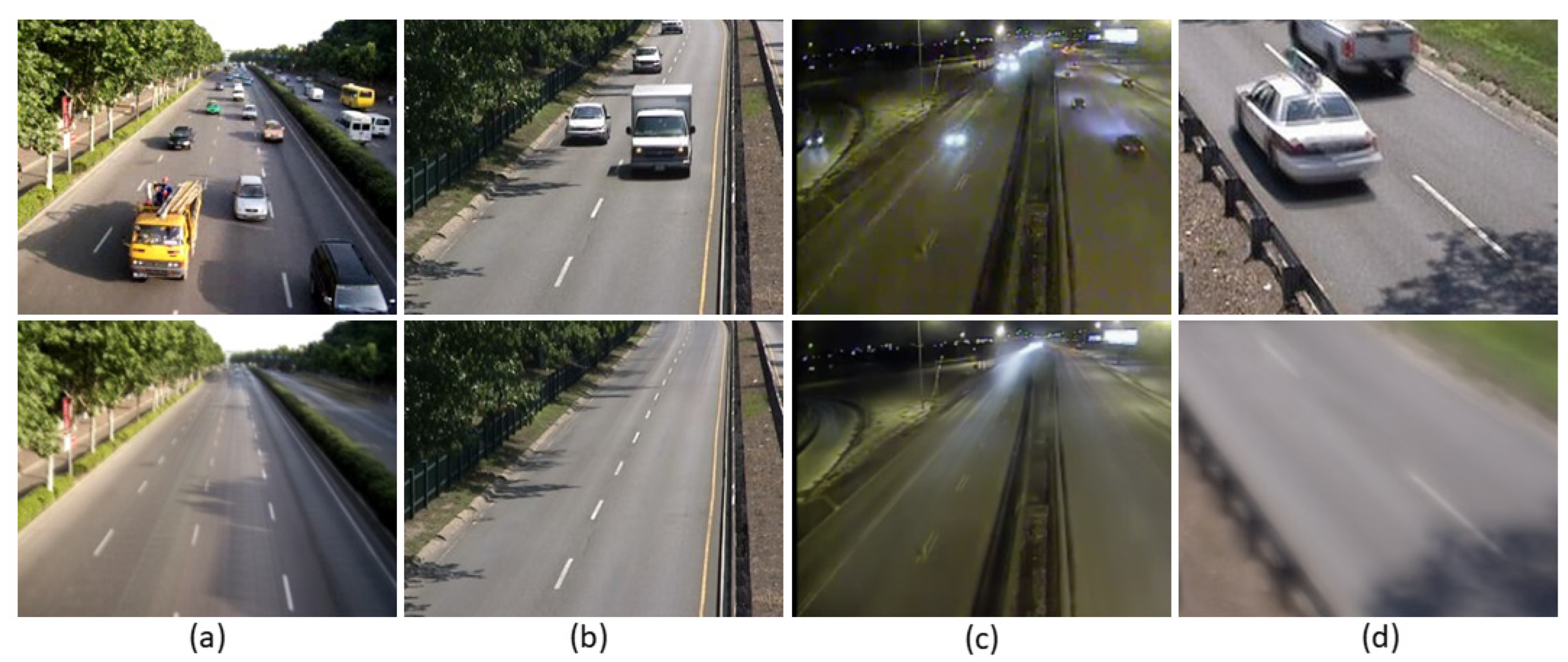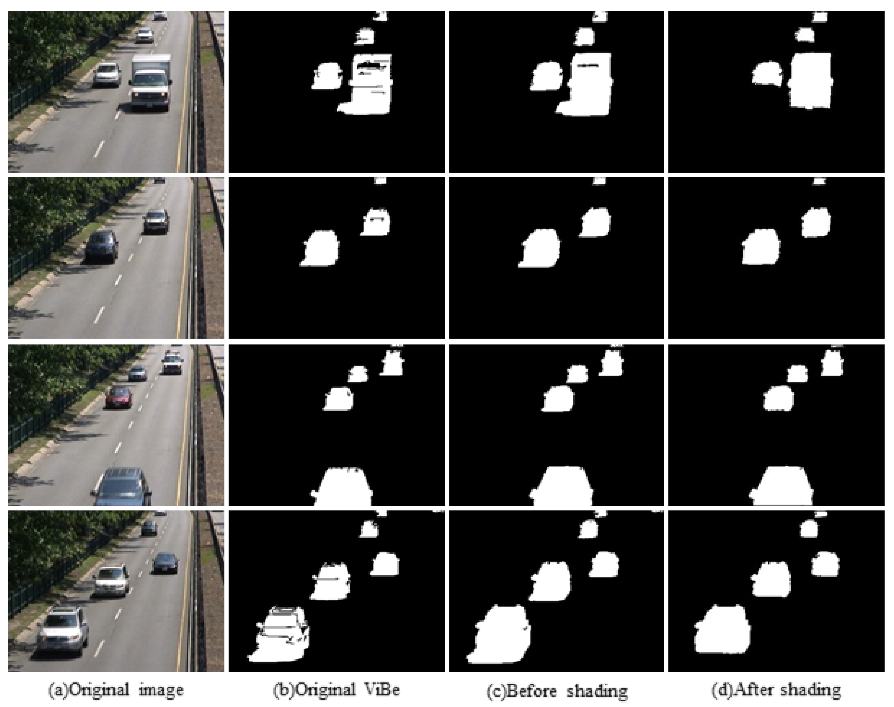Conversely, when the value of $S$ is 0, it means that the more significant the correlation between the current frame and the background frame, it is more likely to be judged as the background, and the effect of the improved moving vehicle target extraction algorithm is shown in Figure 9. Ability to remove shadow effects on the foreground of moving vehicles is shown below.

4. Experimental Results and Analysis

4.1. Experimental Preparation and Experimental Steps

The vehicle detection experiment used the UA-DETRAC dataset [26], which consists of over 140,000 frames with annotations of more than 8000 vehicle objects in Beijing and Tianjin, China. The dataset covers diverse traffic scenarios including highways and road intersections, and vehicle categories are classified into two types: buses and cars. The weather conditions in the dataset include sunny, cloudy, rainy, and night conditions, making it suitable for simulating various traffic scenarios for vehicle detection research.

A self-built test dataset for vehicle detection was created by collecting video data at the overpass in the east section of Xi’an’s Second Ring Road East, which mimics the surveillance video shooting perspective. The dataset comprises of 1200 images and includes sunny, cloudy, and rainy weather conditions. The vehicle categories are classified into cars and buses, and the labeling was performed using LabelImg. XML labeling files were generated to show the category and corresponding positions of the vehicle targets, followed by the normalization of the vehicle coordinates into txt files, with the car and bus categories represented by numbers 0 and 1, respectively.

Experimental platform: The network model training and model testing were performed using the cloud platform AUTODL, 7-core Intel(R) Xeon(R) CPU E5-2680 v4 @ 2.40 GHz CPU, 12 G 3060 RTX GPU, Pytorch1.9.0, Python3.8, CUDA11.1, and the network training parameters were configured as shown in

Table 1. Network training parameters configuration.

Input Image Size	640 × 640	Momentum	0.937
Optimizer	SGD	Weight decay	0.0005
lr0	0.01	Batch size	16
lrf	0.2	Epochs	500

.

The experimental steps are as follows:

(1)

To improve the analysis of vehicle contours via the network, vehicle feature extraction is conducted on the CDnet dataset using a moving vehicle target extraction method.

(2)

The annotated images and self-built datasets, which have undergone vehicle profile feature extraction, are labeled with .xml files that are converted into .txt files to augment the UA-DETRAC dataset.

(3)

A lightweight version of the YOLOv5 model was built and the hyperparameters were tuned for training. The network was trained on the UA-DETRAC and self-built datasets using transfer learning, and the performance was evaluated using mean average precision (mAP) and frame per second (FPS).

(4)

Visualization experiments were conducted on two datasets: the public UA-DETRAC dataset and a self-built dataset.

4.2. Evaluation Indicators

To quantitatively compare the performance of the models, three evaluation metrics, namely precision, recall, and mean average precision (mAP), are utilized. In this experiment, all motor vehicles, including cars and buses, are considered as positive samples, while non-motor vehicles are considered as negative samples. If the real target is a positive sample, the detection result is also a positive sample as $N_{TP}$, the detection result is a negative sample as $N_{FP}$; if the real target is a negative sample, the detection result is also a negative sample as $N_{FN}$, whereas the detection result is a positive sample as $N_{TN}$.

$$\mathrm{Pr}=\frac{N_{TP}}{N_{TP}+N_{FP}}$$

(17)

$$\mathrm{Re}=\frac{N_{TP}}{N_{TP}+N_{FN}}$$

(18)

$$\mathrm{m}AP=\frac{{\displaystyle {\displaystyle \sum }_{j=1}^m}{\displaystyle {\displaystyle \sum }_{i=1}^{n-1}}\left(r_{i+1}-{\mathrm{r}}_{\mathrm{i}}\right)p\left(r_{i+1}\right)}{\mathrm{m}}$$

(19)

where ${\mathrm{r}}_{\mathrm{i}}$ represents the recall corresponding to the ith precision in ascending order, $m$ represents the number of categories of samples in the dataset, which is set to 2 in this experiment.

4.3. Comparison Experiment

4.3.1. Comparison of Effects before and after Data Set Expansion

The experimental dataset includes the UA-DETRAC dataset, the self-built dataset, and the processed CDnet dataset. To demonstrate the effectiveness of the expanded dataset, both the original YOLOv5 model and the improved YOLOv5 model were trained on the standard dataset and the expanded dataset. Three evaluation metrics were used to compare the performance of the two models, namely precision, recall, and mean average precision. Additionally, the training time was also recorded to examine the impact of dataset expansion. The experimental results are shown in

Table 2. Comparison of metrics before and after expanding the dataset.

Epoch	Selection of Data Sets	Model	Pr	Re	AP@0.5	Time (h)
100	Standard data sets	Origin YOLOv-5s	0.9178	0.9147	0.9351	4.43
		Proposed	0.9356	0.9273	0.9467	5.23
	Extended dataset	Origin YOLOv-5s	0.9254	0.9157	0.9343	4.72
		Proposed	0.9334	0.9253	0.9462	5.64
300	Standard data sets	Origin YOLOv-5s	0.9286	0.9206	0.9434	13.28
		Proposed	0.9425	0.9335	0.9725	15.71
	Extended dataset	Origin YOLOv-5s	0.9354	0.9219	0.9493	14.17
		Proposed	0.9638	0.9506	0.9832	16.92
500	Standard data sets	Origin YOLOv-5s	0.9354	0.923	0.9485	22.16
		Proposed	0.9486	0.9387	0.9754	26.15
	Extended dataset	Origin YOLOv-5s	0.9415	0.9263	0.9527	23.65
		Proposed	0.966	0.951	0.987	28.23

.

The experimental dataset consisted of the UA-DETRAC dataset, the self-built dataset, and the processed CDnet dataset. To demonstrate the benefits of expanding the dataset on network training, the original YOLOv5 and the improved YOLOv5 were trained on both the standard dataset and the expanded dataset. Precision, recall, average precision, and training time were used as evaluation metrics. From the results, it can be observed that the extended dataset showed significant advantages over the standard dataset when the number of epochs was increased. Specifically, when training on the extended dataset for 300 epochs, the precision increased by 0.0304, the recall increased by 0.0253, and the average precision increased by 0.037, compared to 100 epochs of training. When training for 500 epochs, the precision increased by 0.0022, the recall increased by 0.0004, and the average precision increased by 0.0038, compared to 100 epochs of training. It is noteworthy that the benefits of expanding the dataset are not significant when the number of epochs is small. Hence, we chose to train the improved YOLOv5-s model on the expanded dataset for 500 epochs to achieve optimal performance.

4.3.2. CA Module Fusion Comparison Experiment

In this paper, we propose three attention mechanism fusion methods. To test the advantages and disadvantages of the three models’ detection effects, we train the original YOLOv5 model on the extended dataset using the parameter configurations listed in Table 1. The results of the three fusion experiments of CA and Li are shown in

Table 3. Comparison of results of fusion CA.

Model	Pr	Re	AP@0.5
YOLOv5-s	0.9215	0.9263	0.9527
YOLOv5-B	0.9277	0.9166	0.962
YOLOv5-N	0.9541	0.9498	0.9729
YOLOv5-H	0.9138	0.9199	0.941

.

The proposed CA module can improve the network’s feature extraction capability by maintaining feature location information and suppressing irrelevant features. However, its effectiveness varies depending on the location. Compared to the original YOLOv5 model, YOLOv5-B improves precision by 0.0062 and mean average precision by 0.0093 but recall decreases by 0.0097. YOLOv5-N achieves the highest average precision among the four models, with precision, recall, and average precision improved by 0.0326, 0.0235, and 0.0202, respectively, compared to the original YOLOv5. In contrast, YOLOv5-H’s precision, recall, and average precision are slightly lower than the original YOLOv5, and it has increased computation cost.

The experimental results indicate that the precision, recall, and average precision are not effectively improved by adding the attention mechanism to any position in the network. In the backbone, a large number of image features are extracted with slight redundancy, and the attention mechanism can help the network perform better feature analysis. However, the feature maps of different scales are not integrated, resulting in insufficient feature extraction and a failure to improve the recall rate. In the neck network, features are integrated from the bottom to the deep layer and from the deep to the shallow layer, allowing for better feature extraction and reconstruction through the attention mechanism for channel attention. This improves the network’s precision rate, recall rate, and mean average precision. In the prediction stage, a large portion of the features are lost, making it difficult for the attention mechanism to distinguish important information from the highly fused feature map, resulting in reduced performance in all three indicators. Based on the experimental results, YOLOv5-N is the optimal choice.

4.3.3. YOLOv5 Ablation Experiment

In this experiment, the extended dataset was partitioned into training and testing sets in an 8:2 ratio. A sequence of ablation experiments was conducted to validate the effectiveness of three proposed enhancements. Ghostnet, DIoU-NMS, and CA modules were incrementally incorporated to analyze their benefits. The experiments were conducted without utilizing pre-trained weights, and the parameters were uniformly configured as described in Table 1. The experimental outcomes are presented in

Table 4. YOLOv5 ablation experiment.

Model	Pr	Re	AP@0.5	AP@0.5:0.95	Model Size
YOLOv5-s	0.9215	0.9263	0.9527	0.8174	13.7 MB
YOLOv5-s + GhostNet	0.9263	0.9292	0.9536	0.8214	10.1 MB
YOLOv5-s + DIoU-NMS	0.9377	0.9366	0.972	0.8286	13.7 MB
YOLOv5-s + CA	0.9541	0.9498	0.9729	0.8339	14.4 MB
YOLOv5-s + Above Three	0.966	0.951	0.987	0.843	10.8 MB

.

In this experiment, the extended dataset is split into a training set and a test set in an 8:2 ratio. To verify the effectiveness of the two proposed improvements, ablation experiments are conducted on the dataset, and GhostNet, DIoU-NMS, and CA modules are sequentially added to analyze their benefits. The experiments do not use pre-training weights, and the parameters are uniformly set as shown in Table 1. The experimental results demonstrate that the original YOLOv5-s achieves a mean precision, recall, and average precision of 0.9215, 0.9263, and 0.9427, respectively. The CA module performs the best, significantly improving the precision and average precision. The improvement effect of DIoU-NMS is slightly weaker, and the GhostNet module does not improve the detection performance but reduces the network parameters. Therefore, the three improvement methods have different focuses. The attention mechanism can enhance the network’s feature extraction ability and focus on extracting essential features. GhostNet reduces the redundancy of the feature map in the convolution operation. DIoU-NMS accurately selects the prediction frame, which can solve the problem of missed detection in the case of vehicle occlusion. Moreover, the introduction of GhostNet, DIoU-NMS, and CA can reduce the number of network parameters, improve inference speed, and enhance the three indicators simultaneously.

To visualize the optimization of DIoU-NMS for detection results, we used the original YOLOv5-s algorithm and the algorithm with the addition of DIoU-NMS to visualize some of the test results using the expanded dataset under the uniform configuration described above. The results are shown in Figure 10.

Figure 9a displays the partial detection results of the original YOLOv5-s algorithm. Missed detection occurs at markers 1 and 2 when there is vehicle obstruction or when the vehicle outline is incomplete. False detection occurs at markers 3, 4, and 5, and the NMS fails to return the correct position of the vehicle, resulting in some detection frames having low accuracy and failing to completely cover the vehicle or exceeding the boundary of the image. Figure 9b shows partial detection results with the addition of the DIoU-NMS structure, which effectively resolves missed detection and false detection in complex vehicle scenarios while ensuring high detection accuracy.

4.3.4. Comparison Experiments and Visualization of Different Models

To evaluate the effectiveness of the proposed algorithm, this study performs cross-sectional comparison experiments on the expanded dataset using five models, namely Faster-RCNN, YOLOv3, YOLOv3-tiny, YOLOv4, and YOLOv4-tiny. The experiments use the configuration parameters listed in Table 1.

The experimental results, as shown in

Table 5. Comparison of different models.

Model	AP@0.5	Frame Time	FPS	FLOPs	Model Size
Faster-RCNN	0.9035	54 ms	18.51	201.07 GFLOPS	309 MB
YOLOv3	0.9341	29.06 ms	34.41	141 GFLOPS	124.4 MB
YOLOv3-tiny	0.8443	15.31 ms	65.32	23.64 GFLOPS	18.9 MB
YOLOv4	0.9478	41.11 ms	24.321	168.56 GFLOPS	245.6 MB
YOLOv4-tiny	0.8934	23.66 ms	42.26	36.34 GFLOPS	25.8 MB
Proposed	0.987	14 ms	71.42	11.6 GFLOPS	10.8 MB

, demonstrate that the algorithm proposed in this paper reduces computation and network parameter overhead, achieves a fast inference speed, and maintains high average precision. Compared with the other five models, it is more suitable for deployment in computing power-limited environments and can provide sufficient preparation for subsequent intelligent transportation systems on lower embedded terminals.

The detection results of the improved model are visualized in experiments to demonstrate the effectiveness. The detection result graphs for the UA-DETRAC and self-built datasets are shown for five scenarios: peak period, flat peak period, low peak period, nighttime, and cloudy and rainy days, as shown in Figure 11. Compared to the original model, the improved model can effectively solve the problem of vehicle leakage and false detection in the vehicle intensive peak period, and the target box regression is closer to the vehicle target. In the night scene, the detection performance is reduced due to the influence of light. Combined with the ablation experiment of Section 4.3.3, it can be concluded that the improved model performs well in the proposed five scenarios and has apparent advantages compared to the original network.

From Figure 11, it can be observed that in the dense traffic scenario during peak hours, the improved model can effectively detect small target vehicles in both the standard and self-built datasets at Conf = 0.25, IoU = 0.45, ensuring high detection accuracy and precision. During periods of plateau and low-demand, the improved model can detect vehicles that produce false images due to the fast vehicle speed. In rainy and night-time scenarios, detection becomes challenging due to the impact of weather and lighting conditions, resulting in varying degrees of missed detection and false alarms for both the original and improved networks. However, the improved network has an overall lower false detection rate and missed detection rate for small, distant targets and vehicle occlusion, demonstrating significant advantages over the original network.

5. Conclusions and Future Work

In this study, an enhanced YOLOv5-s model is proposed for detecting vehicle targets in traffic surveillance. To address the issues of a large number of model parameters and a slow estimate speed, we replaced the CSP structure in the original model with the GhostNet structure and used the SPPF structure to replace SPP, resulting in a reduction in redundant feature parameters and a faster inference speed. Furthermore, we used DIoU-NMS non-great suppression instead of the original NMS to improve localization accuracy and effectively reduce missed and false detections. Additionally, three attention mechanisms were proposed, and comparison experiments were conducted to test the effects of CA attention mechanisms at different locations on detection performance. Finally, the FFD-ViBe algorithm and MD-SILBP operator were combined to extract vehicle features, and the feature maps were used to expand the dataset, enhancing feature extraction. Experimental results show that the proposed method improved the accuracy of the original YOLOv5 by 3.63%, the recall rate by 2.4%, and the average accuracy by 2.2%, indicating that using traditional foreground target extraction to assist the YOLOv5 model for training can effectively improve the detection effect in peak, flat, low, rainy, and night scenarios. Visualization results showed that the proposed algorithm can effectively reduce the rate of missed detections and false detections. Nonetheless, future work will focus on improving the detection of small target vehicles in dense scenes and enhancing the foreground extraction method to obtain more complete vehicle appearance features.

References

1. Yu, B.; Li, J.; Xie, Y. The current situation and problems of intelligent transportation in China. J. Munic. Technol. 2022, 40, 62–66. [Google Scholar]
2. Sun, D.; Roth, S.; Black, M. Secrets of optical flow estimation and their principles. In Proceedings of the IEEE Computer Society Conference on Computer Vision and Pattern, San Francisco, CA, USA, 13–18 June 2010; pp. 2432–2439. [Google Scholar]
3. Qiu, L.; Liu, Q.; Lei, W. Motion detection based on background subtraction fused with three-frame differencing. J. Hefei Univ. Technol. 2014, 37, 572–577. [Google Scholar]
4. Lai, L.; Xu, Z.; Zhang, X. Improved Gradient Optical Flow Method Applied in Image Stabilization System. Infrared Laser Eng. 2016, 45, 280–286. [Google Scholar]
5. Wang, J.; Zhang, Q. Background Modeling and Moving Object Detection Based on Frame Difference and Gaussian Mixture Model. Electron. Des. Eng. 2019, 27, 16–19. [Google Scholar]
6. Yin, Y.; Yang, T.; Wang, Y. Adaptive Background Modeling and Detection Method for Moving Objects from Car Cameras. Optoelectron. Laser 2019, 30, 864–872. [Google Scholar]
7. Simonyan, K.; Zisserman, A. Very Deep Convolutional Networks for Large-Scale Image Recognition. arXiv 2014, arXiv:1409.1556. [Google Scholar]
8. Xu, T.; Lin, L.; Shen, S. Scale-Aware Fast R-CNN for Pedestrian Detection. IEEE Trans. Multimed. 2018, 20, 985–996. [Google Scholar]
9. Jiang, H.; Learned-Miller, E. Face detection with the faster R-CNN. In Proceedings of the 12th IEEE International Conference on Automatic Face & Gesture Recognition (FG 2017), Washington, DC, USA, 30 May–3 June 2017; pp. 650–657. [Google Scholar]
10. Cao, G.; Xie, X.; Yang, W. Feature-fused SSD: Fast detection for small objects. In Proceedings of the Ninth International Conference on Graphic and Image Processing (ICGIP 2017), Qingdao, China, 10 April 2018; pp. 381–388. [Google Scholar]
11. Wong, A.; Famuori, M.; Shafiee, M.J. Yolo nano: A highly compact you only look once convolutional neural network for object detection. In Proceedings of the 2019 Fifth Workshop on Energy Efficient Machine Learning and Cognitive Computing-NeurIPS Edition (EMC2-NIPS), Vancouver, BC, Canada, 13 December 2019; pp. 22–25. [Google Scholar]
12. Zhou, H.; Zhang, Q.; Liu, Y. Face Detection Method Based on YOLO2 for Subway Passenger Flow into Station. Comput. Mod. 2019, 10, 76–82. [Google Scholar]
13. Mao, Q.; Sun, H.; Liu, Y. Mini-YOLOv3: Real-time object detector for embedded applications. IEEE Access 2019, 16, 133529–133538. [Google Scholar] [CrossRef]
14. Dewi, C.; Chen, R.; Liu, Y. I Yolo V4 for advanced traffic sign recognition with synthetic training data generated by various GAN. EEE Access 2021, 9, 97228–97242. [Google Scholar] [CrossRef]
15. Kuznetsova, A.; Maleva, T. Detecting apples in orchards using YOLOv3 and YOLOv5 in general and close-up images. Int. Symp. Neural Netw. 2020, 12557, 5390–5406. [Google Scholar]
16. Wang, Y.; Wang, F.; Sun, Q. Multi-Scale Feature Fusion Vehicle Detection Method. J. Syst. Simul. 2022, 34, 1219–1229. [Google Scholar]
17. Li, Y.; Ma, R.; Zhang, M. Improve the monitoring video traffic flow statistics of YOLOv5s+DeepSORT. Comput. Eng. Appl. 2022, 58, 271–279. [Google Scholar]
18. Lu, X.; Ling, H. Real-time Multiple-vehicle Detection and Mracking from A Moving Platform. IEEE Trans. Intell. Transp. Syst. 2017, 18, 3473–3483. [Google Scholar]
19. Meng, D.; Xiang, S.; Pan, C. Tracking-by-detection of Vehicles in UAV Videos Using Deep Learning and Motion Cues. Comput. Vis. Image Underst. 2020, 198, 103015. [Google Scholar]
20. Han, K.; Wang, Y.; Tian, Q.; Guo, J.; Xu, C.; Xu, C. Ghostnet: More features from cheap operations. In Proceedings of the IEEE/CVF Conference on Computer Vision and Pattern Recognition, Seattle, WA, USA, 13–19 June 2020; pp. 1580–1589. [Google Scholar]
21. He, K.; Zhang, X.; Ren, S. Spatial pyramid pooling in deep convolutional networks for visual recognition. IEEE Trans. Pattern Anal. Mach. Intell. 2015, 37, 1904–1916. [Google Scholar] [CrossRef] [Green Version]
22. Gu, R.; Wang, G.; Song, T. CA-Net: Comprehensive attention convolutional neural networks for explainable medical image segmentation. IEEE Trans. Med. Imaging 2020, 40, 699–711. [Google Scholar] [CrossRef]
23. Feng, Z.; Wang, X.; Yang, Z. An Improved ViBe Algorithm of Moving Target Extraction for Night Infrared Surveillance Video. KSII Trans. Internet Inf. Syst. (TIIS) 2021, 15, 280–286. [Google Scholar]
24. Liu, Y.; Zeng, T.; Chen, D. Research on Motion Target Detection Based on Improved ViBe Algorithm. Comput. Simul. 2019, 36, 280–286. [Google Scholar]
25. Kalirajan, K.; Sudha, M. Moving object detection using median-based scale invariant local ternary pattern for video surveillance system. J. Intell. Fuzzy Syst. 2017, 33, 1933–1943. [Google Scholar] [CrossRef]
26. Sahu, C.K.; Young, C.; Rai, R. Artificial intelligence (AI) in augmented reality (AR)-assisted manufacturing applications: A review. Int. J. Prod. Res. 2021, 59, 4903–4959. [Google Scholar] [CrossRef]
Figure 1. The structure of the YOLOv5.
Applsci 13 04088 g001
Figure 2. The structure of the Ghost model.
Applsci 13 04088 g002
Figure 3. The structure of the multi-scale integration.
Applsci 13 04088 g003
Figure 4. The structure of the CA mechanism.
Applsci 13 04088 g004
Figure 5. YOLOv5_B network structure.
Applsci 13 04088 g005
Figure 6. YOLOv5_N network structure.
Applsci 13 04088 g006
Figure 7. YOLOv5_H network structure.
Applsci 13 04088 g007
Figure 8. (ad) Background modeling of four scenarios.
Applsci 13 04088 g008
Figure 9. Partial comparison chart of CDnet dataset.
Applsci 13 04088 g009
Figure 10. Comparison of original and added DIoU-NMS networks ((a) for the original network; (b) for added DIoU-NMS network).
Applsci 13 04088 g010
Figure 11. Comparison of original model results (b,e) and optimized model results (c,f) for two datasets: (a,d).
Applsci 13 04088 g011