Real-Time Target Detection System for Animals Based on Self-Attention Improvement and Feature Extraction Optimization

Abstract

In this paper, we propose a wildlife detection algorithm based on improved YOLOv5s by combining six real wildlife images of different sizes and forms as datasets. Firstly, we use the RepVGG model to simplify the network structure that integrates the ideas of VGG and ResNet. This RepVGG introduces a structural reparameterization approach to ensure model flexibility while reducing the computational effort. This not only enhances the ability of model feature extraction but also speeds up the model computation, further improving the model’s real-time performance. Secondly, we use the sliding window method of the Swin Transformer module to divide the feature map to speed up the convergence of the model and improve the real-time performance of the model. Then, it introduces the C3TR module to segment the feature map, expand the perceptual field of the feature map, solve the problem of backpropagation gradient disappearance and gradient explosion, and enhance the feature extraction and feature fusion ability of the model. Finally, the model is improved by using SimOTA, a positive and negative sample matching strategy, by introducing the cost matrix to obtain the highest accuracy with the minimum cost. The experimental results show that the improved YOLOv5s algorithm proposed in this paper improves mAP by 3.2% and FPS by 11.9 compared with the original YOLOv5s algorithm. In addition, the detection accuracy and detection speed of the improved YOLOv5s model in this paper have obvious advantages in terms of the detection effects of other common target detection algorithms on the animal dataset in this paper, which proves that the improved effectiveness and superiority of the improved YOLOv5s target detection algorithm in animal target detection.

1. Introduction

Target identification for the recognition of wild animals has developed into one of the main applications in the current computer vision area due to the maturity of the technology in that field. Still, the current common methods do not obtain satisfactory requirements. Deep learning has emerged as a groundbreaking technology in this area, and it is employed frequently due to its high target identification speed and accuracy [1,2].

Increasing human enterprises have led to a result that nature’s resources are being exploited more and more, and the habitats of wild animals are becoming less and less available, and it is increasingly difficult to find them in nature. Continuous target detection research has aided the study of animal detection and identification in recent years, which is crucial for preventing the extinction of some wild creatures [3,4].

The YOLO (You Only Look Once) algorithm [5,6] provides a faster method of detection. In the CNN, regression and classification are carried out directly on the entire graph since the YOLO algorithm directly regresses the position of the bounding box and the category to which it belongs in the output layer and is trained and identified in a separate network [7,8]. YOLOv1 used one network to output the position and category, applying the one-stage processing [9]. In order to increase identification speed and minimize the number of convolutional layers, YOLOv2 recommended combining datasets with a new network called Darknet-19 [10]. In YOLOv3, the new network, Darknet-53, was applied for feature extraction [11]. YOLOv4 proposed Mosaic data enhancement and used the SPP module, DIOU NMS, for optimization [12]. In June 2020, YOLOv5 was proposed [13]; it used the Focus module for optimization, and algorithms such as YOLOv5s, YOLOv5m, YOLOv5l, and YOLOv5x appeared. Many scholars have devoted themselves to combining YOLO target detection algorithms with practical engineering applications, showing the power of YOLO algorithms [14].

To extract more precise and thorough semantic characteristics, Farzaneh Dadrass Javan et al. studied the enhanced YOLOv4 algorithm by altering the system’s convolutional layer count [15]. Using a shallow feature improvement mechanism and a wraparound box uncertainty prediction mechanism, Wang Qingyan et al. studied the enhanced YOLOv4 algorithm. The network’s features were extracted using the shallow feature enhancement mechanism, and the network’s capacity to localize small targets and the color resolution were increased by combining the shallow features from two stages with the high-level semantic features discovered after two rounds of upsampling [16]. The ECA-Net mechanism was added by Xin Li et al. to the backbone’s end to enhance the extraction of model features. Subsequently, the BiFPN module was introduced to enhance the PANet structure of the backbone. At the same time, the fusion of model features was enhanced to address the issue of the conventional detection methods for aero-engine parts indicating defects’ sluggish speed and low accuracy [17]. The BottleneckCSP module is replaced by the BottleneckCSP-2 to identify apples veiled by obscurants module developed by Bin Yan et al. in the original YOLOv5s network backbone design. Additionally, the enhanced backbone suggested in this research was added, leading to a higher mAP and the SE module from the visual attention mechanism network [18].

Xiaohan Ding et al. proposed a RepVGG convolutional neural network, which consists of 3*3 convolutional layers and ReLU. The decoupling of RepVGG is achieved by the structural reparameterization technique. Since it does not concern about the number of parameters, RepVGG is more parameter efficient than ResNets, showing the power of RepVGG compared to models such as EfficientNet and RegNet [19]. Swin Transformer, a brand-new visual transformer, was suggested by Ze Liu et al. This study suggests a hierarchical Transformer whose computation of its representation uses shifted windows, which improves the flexibility of the algorithm and as well as reduces the algorithm’s computation, and greatly improves its efficiency, and its effectiveness on the COCO testdev target detection task further demonstrates the effectiveness of the Swin Transformer [20]. Solving OT problems using the Sinkhorn–Knopp method results in 25% more training time, according to Zheng Ge’s new high-performance YOLO algorithm, YOLOX. As a consequence, they reduce the complexity of the Sinkhorn–Knopp algorithm to a dynamic top-k strategy, commonly known as SimOTA, a technique for positive and negative sample matching. This paper introduces a formula of cost, which calculates its minimum cost in the labeled region, making a better balance of algorithm accuracy and speed [21]. By applying the multi-headed self-attentive module and position coding in [22] and [23] to the algorithm of computer vision, the C3TR module emerges. The C3TR module is obtained by replacing the original Bottleneck with the TransformerBlock module based on the C3 structure. In order to improve the detection effect of occluded targets, the C3TR module with TransformerBlock is used to replace the BottleneckCSP module.

In this paper, YOLOv5s is improved to better apply YOLOv5s to wildlife target detection. This paper first introduces RepVGG lightweight network structure in the backbone to enhance the feature extraction capability of animal targets in the natural environment dataset of this paper, which enhances the model’s adaptability and detection speed. This improves the detection accuracy and speed of the YOLOv5s algorithm. Secondly, some C3 modules of the backbone and head are replaced by Swin Transformer modules, which use sliding windows to divide the feature maps and improve the computational speed and efficiency at the cost of minimizing the perceptual field loss. The C3TR module is then used to enlarge the feature map’s perceptual field in place of the head’s C3 module. Then, SimOTA is employed as a technique for matching positive and negative samples, and a cost function is added to reduce loss during training. As a result, the model’s computation is simplified, the training period is shortened, and the YOLOv5s network’s detection speed is increased. Depending on the experimental findings, the model has increased detection accuracy and speed, making it more suitable for use on edge devices and capable of fully detecting and identifying wild animals in their natural habitat.

2. YOLOv5 Algorithm

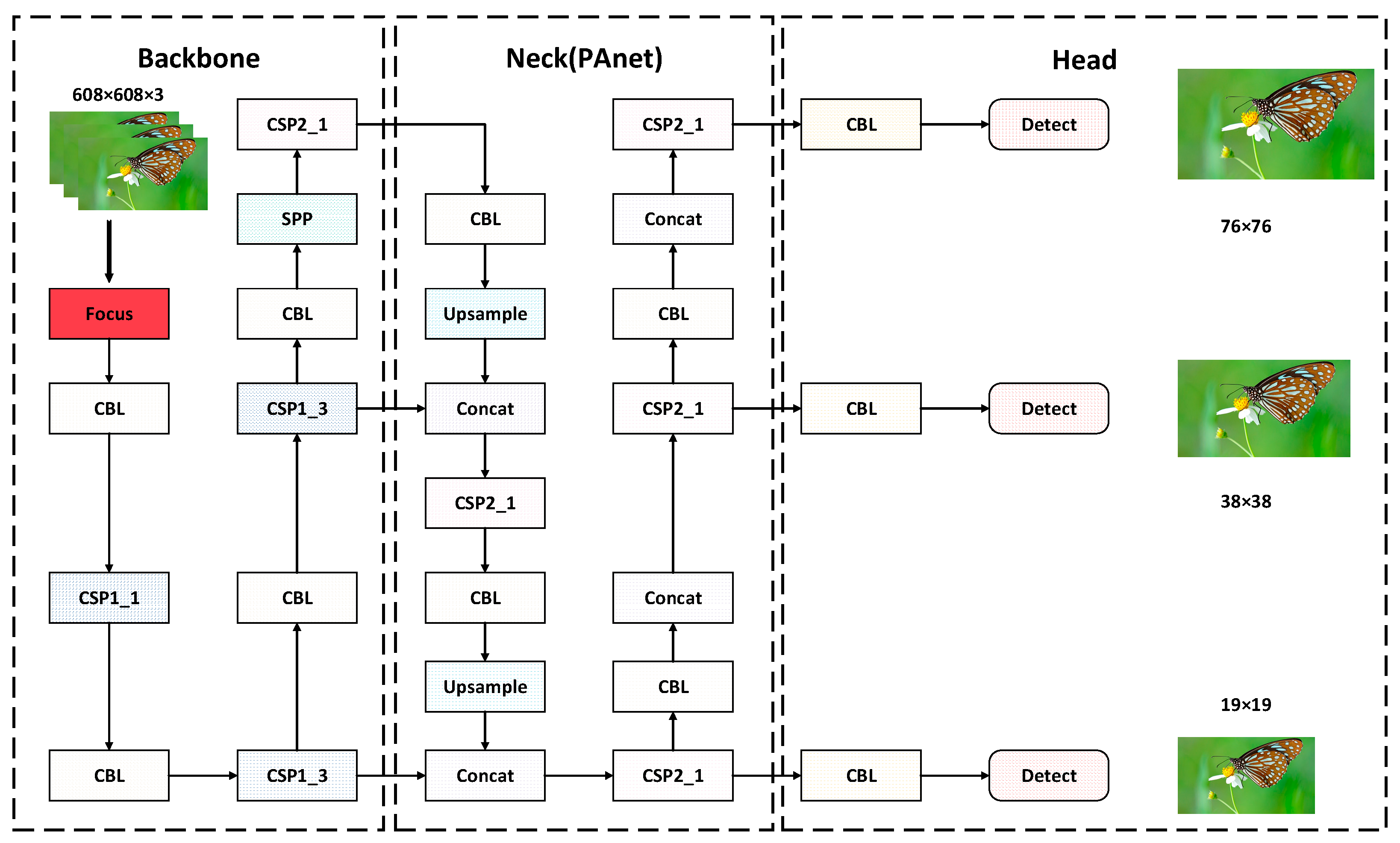
Input, Backbone, Neck, and Prediction are the four primary components of YOLOv5, and Figure 1’s network topology depicts these components. YOLOv5 has four different network models: YOLOv5s, YOLOv5m, YOLOv5l, and YOLOv5x. In this paper, YOLOv5s is chosen as the base architecture [24].

YOLOv5 uses bi-trivial interpolation on the input side to fix the image size, uses Mosaic data enhancement, and solves the black edge problem by adaptive scaling. Backbone uses CSPDarknet53 as a feature extraction network, adding a CSP module to enable some features to be connected across stages and extracting the initial image features by spatial pyramid pooling (SPP), reducing the computational effort. Neck creates feature pyramids with various scales and resolutions using the PANet network structure, which consists of a set of top-down and bottom-up paths. PAN creates feature pyramids at various scales by using the feature maps from the Backbone bottom-up and several convolutional layers. FPN adopts top-down feature pyramids and upsamples them to higher resolutions, thus allowing for finer-grained target detection. The multi-scale problem is resolved by using both at the same time, improving the network feature fusion capabilities and the model’s identification of targets of various sizes. The detection head in Prediction is made up of a number of convolutional layers that use three anchor frames for each scale of prediction to determine the location of objects in the image before obtaining the greatest confidence frame by non-maximum suppression [25]. Compared with YOLOv3, YOLOv5 uses Mosaic data augmentation, adaptive anchor frame calculation, adaptive image scaling operations on the Input side and introduces the Focus module and CSP module on the backbone, which makes the model modular and increases the flexibility of the model. In addition, unlike the Darknet framework used in YOLOv4, the Pytorch framework used in YOLOv5 makes it easier for others to train their own datasets on YOLOv5. YOLOX is similar to YOLOv5s in terms of network structure. YOLOX also uses the Focus module and CSPDarknet on backbone53, and uses FPN + PAN structure like YOLOv4 and YOLOv5.

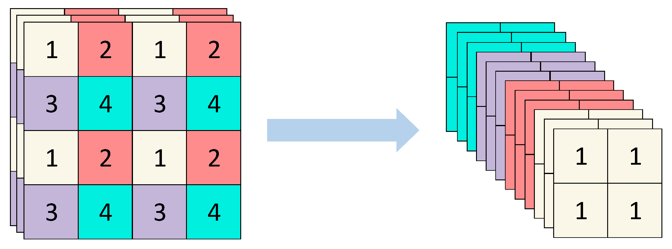
Focus downsampling is the main feature that distinguishes YOLOv5 from YOLOv4, mainly by slicing the higher-resolution image into multiple lower-resolution feature maps [26]. Focus expands the input channels by a factor of 4, which can increase the computational power of the network while preventing information loss, and then slices the image. As shown in Figure 2, the 4 × 4 × 3 image is firstly sliced into four parts, and then stitched into a 2 × 2 × 12 feature map in channel dimension, and then convolved by 3 × 3 to obtain different feature information and output channel 32 to generate a 2 × 2 × 32 feature map [27].

The feature map consists of a convolutional layer, a BN (Batch Normalization) layer, and an activation function layer; CBS is similar to CSP in that it is a composite convolutional module. Among them, the convolution layer is ordinary convolution, and the BN layer introduces normalized activation into the network and normalizes it, which ensures that the input distribution inside the model can be learned by each layer when the model is trained and facilitates fast convergence of the accelerated network. The SiLU function is utilized in YOLOv5s as the activation function, enhancing the model’s performance and allowing for more nonlinear expression. The SiLU function has the following expression:

$$SiLU\left(x\right)=\frac{x}{1+e^{-x}}$$

(1)

The CSP structure is enhanced by YOLOv5 by using C3. It has two channels, one of which uses multiple Bottleneck stacks and three common convolutional layers. The other goes through a convolutional module, and the two channels are then concatenated (concat) and output by Conv. In contrast to the BottleneckCSP module, the SiLU function replaces the activation function in the convolution module after concat. The residuals are removed from the Conv module after the output. The use of the C3 module enhances the feature fusion and feature extraction capabilities, reducing the model size and computation while maintaining the existing detection accuracy and detection speed.

There are three loss functions in YOLOv5, which calculate the classification, location, and confidence loss, respectively [28]. The classification loss determines whether the anchor frame matches the calibrated classification, and the confidence loss determines the network’s confidence; both are typically determined using the binary cross-entropy loss function (BCE With Logits Loss).

$$BC{E}_{Loss}=-\frac{1}{N}{\displaystyle \sum _{i=1}^N{y}_i^{*}\ln y_i+(1-y_i^{*})\ln (1-y_i)}$$

(2)

$$y_i=sigmoid(x_i)=\frac{1}{1+e^{-x_i}}$$

(3)

where N is the total number of categories, $y_i$ is the probability of a category, $y_i^{*}$ is the true value of the category (true is 0; otherwise is 1), and $x_i$ is the predicted value of the category.

The GIoU function is typically used to determine the location loss, which is calculated as the error between the predicted frame and the true frame.

$$GIo{U}_{Loss}=1-GIoU=1-IoU+\frac{|C-A\cup B|}{\left|C\right|}$$

(4)

$$IoU=\frac{|A\cap B|}{|A\cup B|}$$

(5)

where A represents the prediction frame, B represents the true frame, and C is the minimum convex set of A and B. When the prediction and true frames are both empty, it is impossible to calculate the intersection of the two frames. The smaller the value of GIoU, the less the error between the prediction frame and the true frame [29].

3. Improved Algorithm Based on YOLOv5s

For the task requirement of wildlife detection, the YOLOv5s model based on self-attention improvement and feature extraction optimization proposed in this paper will be improved by the RepVGGBlock module, Swin Transformer module, C3TR, and positive and negative sample matching strategy, SimOTA.

3.1. Improvement Based on YOLOv5s and REPVGG Models

The VGG network structure is one of the models used for target recognition that has the drawback of being prone to gradient disappearance and explosion issues. The ResNet network structure’s residual branch addresses the issues of gradient disappearance and explosion, but it is simple to introduce the issue of model overfitting. Given that the original YOLOv5s employs the original convolution as its foundation, increasing the network depth by including additional convolutional layers is a more straightforward way to improve its ability to extract features. This approach will, however, result in the addition of an excessive number of network model parameters, which will increase the YOLOv5s algorithm’s detection accuracy but slow down its detection speed. If we want to improve the detection speed while improving the detection accuracy of the algorithm, we need to replace the original network structure of YOLOv5s with the RepVGG lightweight network structure as the backbone network, i.e., replace the CBS module in the original YOLOv5s with the RepVGGBlock module [30].

RepVGG network is a simple and fast convolutional neural network. Since the RepVGG network structure has fewer convolutional layers and model parameters than the original convolutional network structure, this makes the network computationally faster than the original convolutional neural network. Although there are many other state-of-the-art lightweight network structures available, they still have some shortcomings compared to RepVGG. For example, Mobilenetv2 [31], DenseNet [32], and GhostNet [33], these models increase the computational effort of the model as well as the model size in improving the performance, making such lightweight network models more difficult to deploy to the endpoints. In contrast, the dataset of this paper requires models that are more easily deployed to mobile devices to facilitate the detection of animals, which is why the RepVGG model cannot be replaced. 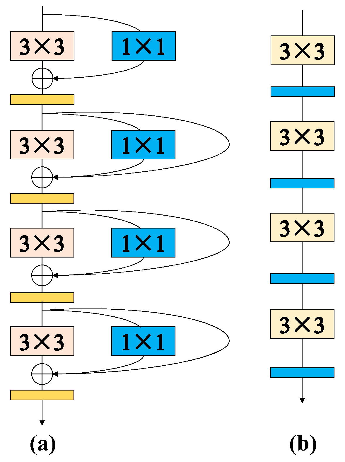The RepVGG network uses different network architectures for training and network inference phases, with the training phase performing network performance improvement and the inference phase focusing on network speed [34]. RepVGG uses a multi-branch model in the training phase and converts it to a single-path model in the inference phase. In the training phase, the RepVGG network contains an Identity residual structure and 3 × 3 convolutional kernels, and 1 × 1 convolutional kernels. The 1 × 1 convolutional branch is introduced in the Block of the VGG network, and then the residual branch is introduced to solve the problem of gradient explosion and gradient disappearance of the model and enhance the feature extraction ability of the algorithm [35]. In the inference stage, the convolutional and BN layers are firstly combined, and then the Conv1 × 1 and residual branches in the network are transformed into Conv3 × 3 with a plain structure by fusion. Figure 3 depicts the network topology for RepVGG training in panel a and the network structure for inference in panel b.

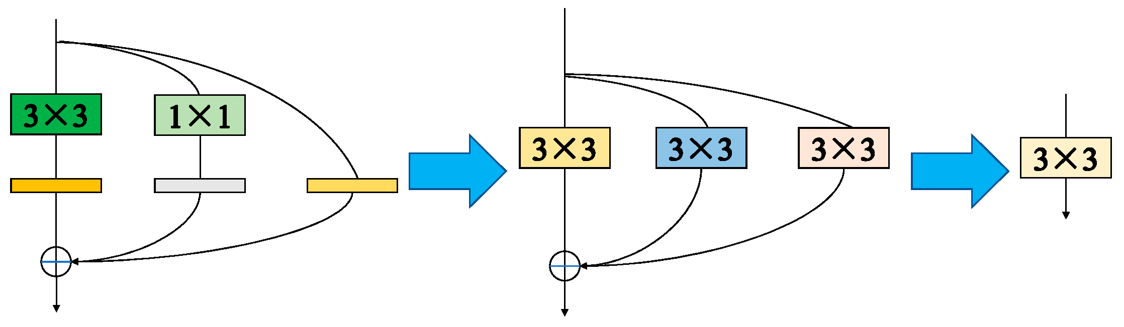
The multi-branch structure in the training process is changed into Conv3 × 3 by reparameterizing the RepVGG structure. The RepVGG network merges the convolutional and BN layers to improve the inference speed of the network by reducing the number of layers and reducing the memory occupation. The BN layer facilitates fast convergence to accelerate the network and effectively solve the gradient disappearance and gradient explosion problems. However, the BN layer occupies more memory and video memory in the forward inference of the network. Figure 4 depicts the structural reparameterization procedure.

Reducing the number of layers in neural networks improves network performance, and convolutional layers are formulated as follows:

$$Conv(x)=W(x)+b$$

(6)

The BN layer formula is as follows:

$$BN(x)=\gamma \cdot \frac{(x-u)}{\sqrt{{\sigma }^2}}+\beta$$

(7)

At this point, we replace the convolution layer formula with the BN layer formula.

$$BN(Conv(x))=\gamma \cdot \frac{(W(x)+b-u)}{\sqrt{{\sigma }^2}}+\beta$$

(8)

This is then reduced to:

$$BN(Conv(x))=\frac{\gamma \cdot W(x)}{\sqrt{{\sigma }^2}}+(\frac{\gamma \cdot (b-u)}{\sqrt{{\sigma }^2}}+\beta )$$

(9)

It can be seen that the right end of Equation (9) is the expression of the convolution layer formula, such that:

$$W_1=\frac{\gamma \cdot W}{\sqrt{{\sigma }^2}}$$

(10)

$$B_1=\frac{\gamma \cdot (b-u)}{\sqrt{{\sigma }^2}}+\beta$$

(11)

The final fusion results in:

$$BN(Conv(x))=W_1(x)+B_1(x)$$

(12)

Since the final convolution is predictable based on the above deductive procedure, we may employ the technique of mixing the Conv and BN layers to speed up the algorithm’s processing. In the RepVGG structure, two branching structures of 1 × 1 convolutional kernel identity are introduced. To add up the convolution kernels, both 1 × 1 convolution and identity need to be transformed into Conv3 × 3. To convert Conv1 × 1 into Conv3 × 3 convolution, first move the convolution kernel to the center of Conv3 × 3, i.e., Conv1 × 1 padding into the form of Conv3 × 3 convolution kernel. In this Conv3 × 3, the original Conv kernel is all zeros. The identity structure can be constructed as a Conv1 × 1 with a weight equal to 1. The weight of the convolution is 1, which ensures that the input is equal to the output. The three convolution branches can then be combined in accordance with the additive property of convolution after the aforesaid procedure converts the Conv1 × 1 kernel into a Conv3 × 3 kernel. Overall, structural reparameterization first merges the convolution kernel with the BN layer, then the three convolutions with the centroid as the reference must be added, and then the three convolutions into one convolution by the additivity of the convolution kernel must be merged. In general, RepVGG incorporates the features of models such as VGG and ResNet. While improving the accuracy, the structural reparameterization can convert the trained model into a single-way structure used for inference deployment in order to avoid bringing complex structures.

3.2. Improvements Based on YOLOv5s and Swin Transformer

The Transformer has been widely used in the field of NLP and has recently migrated to the field of computer vision, where it can be used for target detection, object classification, semantic segmentation, instance segmentation, and other computer vision tasks. The detection targets of this animal dataset are mostly medium-sized targets, so we apply Swin Transformer to this animal dataset, and the experimental results confirm that the application of the Transformer to this animal image block improves the detection accuracy and detection speed of the algorithm.

Transformer was originally used to solve the natural language translation problem, and Vision Transformer [36] was suggested by Alexey Dosovitskiy et al. to use Transformer in the field of computer vision by segmenting an image into multiple image blocks and flattening each image block into a one-dimensional vector to be used as the input of Transformer to train the classification model in a supervised manner. The pre-training results of large data sets show that the accuracy exceeds the highest results of CNN [37,38].

Swin Transformer [39] is a self-attentive mechanism for deep learning models, whose primary goal is to effectively interpret high-resolution images by breaking them up into smaller blocks and using hierarchical attention processes to gather both local and global contextual information. The following equation serves as a summary of the Swin Transformer’s structure:

$$SwinTR=T+S+P+FFN$$

(13)

where T denotes the tokenization layer, S denotes the shifted window mechanism, P denotes the patch merging layer, M denotes the multi-scale architecture, and FFN stands for the feed-forward network. The tokenization layer segments the input image into a series of non-overlapping patches, which are then processed by a shift window mechanism to capture the contextual information of different regions of the image. The patch merging layer combines the features of different patches to create a uniform representation of the image, while the multi-scale architecture helps the model to detect objects of different sizes. Finally, the feedforward network performs the final classification and regression tasks to identify and localize objects in the image. Overall, Swin Transformer uses a sliding window approach to achieve cross-window connectivity in a hierarchical feature map for feature interaction, which can effectively capture local and global contextual information.

Although the C3 module has the global perceptual field of the feature map, it is computationally intensive, which seriously affects the training and detection speed of the model, especially when the input image resolution is high. In this paper, we replace some C3 modules of the backbone and head with Swin Transformer modules, which can improve the computational speed and efficiency at the cost of minimizing the loss of perceptual field by using two window partitioning mechanisms alternately, and this structure has the flexibility of multi-scale modeling and takes into account the efficiency and characterization ability. Since most of the detection objects in this paper are large targets with relatively obvious features, other lightweight networks such as CBAM [40] need to focus on both channel and spatial dimensions to obtain more detailed attention information, which instead increases the number of parameters and computational effort to some extent. The improved Swin Transformer module in this paper has a multiscale architecture that allows flexible switching in the detection of small and large targets, while its unique sliding window mechanism enables cross-window connections in the hierarchical feature map, which can also effectively capture more extensive regional information without affecting the computational speed and efficiency.

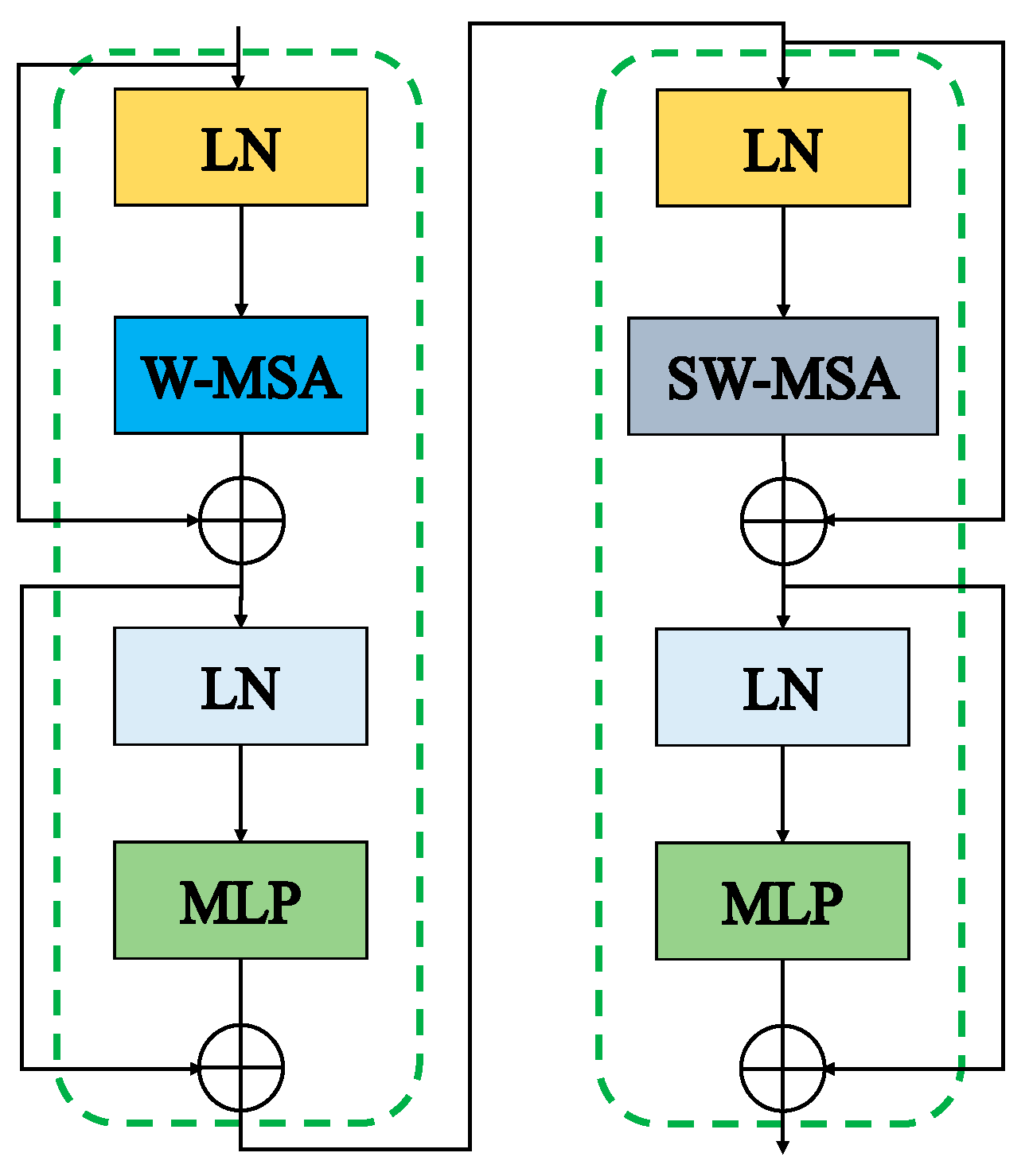
Figure 5 shows two consecutive Swin Transformer modules. While W-MSA is a conventional multi-headed self-attentive module, SW-MSA adds a moving window scheme to W-MSA. This moving window-based self-attentive module allows Swin Transformer to capture remote dependencies between image blocks without using the full attention mechanism between all block pairs, significantly reducing the computational cost of Swin Transformer.

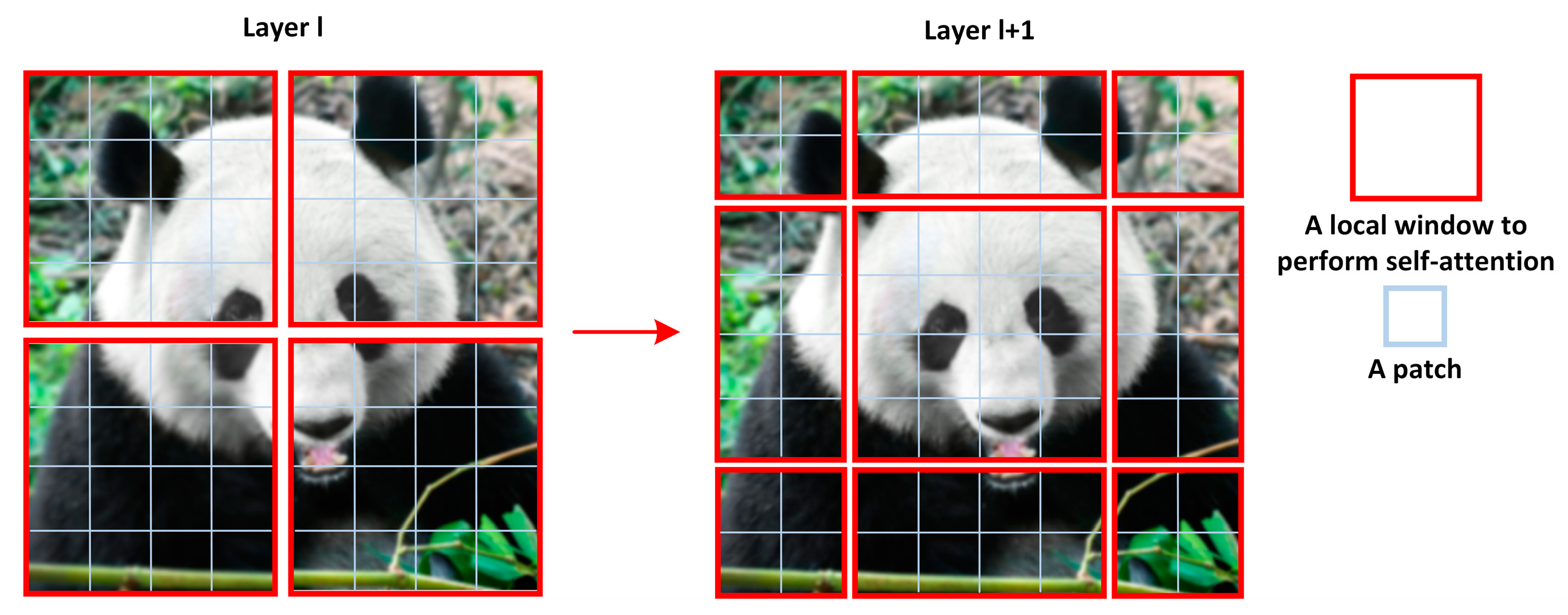
Figure 6 depicts the operation of W-MSA and SW-MSA. As seen in Figure 6 left, W-MSA evenly separates the feature map into four local windows, each of which operates independently and with no information sharing between them. This causes W-MSA to lose the global sensory field when dividing, and each window only receives local feature map information, which will restrict the model’s capacity to extract features. As shown in Figure 6 right, the windows are allowed to move in SW-MSA so that some of the windows can receive information from multiple windows in the upper layer (e.g., the rectangular window in the middle receives information from four windows in the upper layer), which can reduce the loss of the sensory field. In addition, the moving window design provides connections between different windows, which significantly enhances the modeling capability.

Assuming that the image is segmented into n windows, each window has m×m chunks, and MSA and W-MSA have a time complexity of:

$$O(MSA)=4n{C}^2+2n^{2}C$$

(14)

$$O(W-MSA)=4n{C}^2+2m^{2}nC$$

(15)

where C is a constant and m tend to take a constant value (default is 7). Therefore, MSA has quadratic complexity with respect to n, and W-MSA has linear complexity. The computational process between two consecutive Swin Transformer modules can be inscribed by the following equation:

$$\left\{\begin{array}{l}{\widehat{z}}^l=W-MSA(LN(z^{l-1}))+z^{l-1}\\ z^l=MLP(LN({\widehat{z}}^l))+{\widehat{z}}^l\\ {\widehat{z}}^{l+1}=SW-MSA(LN(z^l))+z^l\\ z^{l+1}=MLP(LN({\widehat{z}}^{l+1}))+{\widehat{z}}^{l+1}\end{array}\right.$$

(16)

where $z^l$, ${\widehat{z}}^l$, $z^{l+1}$, ${\widehat{z}}^{l+1}$ denotes the feature map information output by W-MSA, MLP, SW-MSA, and MLP, respectively, and the four are connected sequentially.

Improvement Based on YOLOv5s with C3TR

In practical applications, the size of the detection target is often not fixed, and the C3 module has a weak detection capability and a small feature map field of perception when facing targets of different scales, and at the same time, the feature grid sampled by the C3 module is large, making the FLOPs larger. To solve this problem, the first C3 module of the head is replaced by C3TR and compared with ViT, the feature map is segmented into multiple image blocks, and then each image block is flattened into a one-dimensional vector as input instead of directly segmenting the original image, which not only can make full use of the convolutional network to filter out a lot of irrelevant information of the original image, but also can promote the convergence of the network by extracting feature information as input. By incorporating a multi-head self-attentive mechanism and multi-layer perception, the global self-attentive computation, when compared to C3, can expand the perceptual field of the feature map and has a very good learning ability [41].

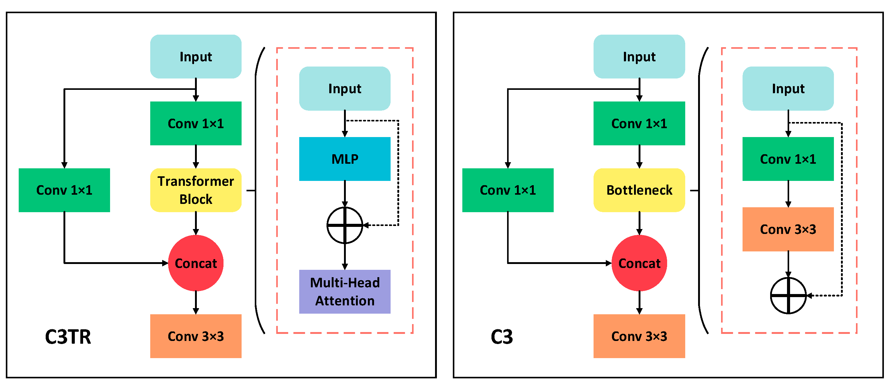
C3TR is a modified C3 module [42], as shown in Figure 7. C3TR replaces the original Bottleneck part with TransformerBlock. TransformerBlock consists of alternately connected multi-headed self-attentive modules (MSA) and multilayer perceptrons (MLP). MSA normalizes the global feature information for linear projection and then non-linearly outputs features by the MLP.

MSA allows parallel processing of sequences of feature map information because each head of MSA can process a different subset of the sequence separately. Each head of MSA computes separately a set of attention weights that determine the dependence of each piece of information in the sequence on the other information and then uses the attention weights to compute a weighted sum of the sequence information, which will produce a new representation of the sequence containing information from all the heads. This mechanism allows MSA to simultaneously acquire surrounding pixel information, expanding the perceptual field of the feature map and reducing false recognition of suspected objects. MLP, on the other hand, enhances the self-attentive mechanism’s representation, allowing better access to contextual information and minimizing the loss of global information. TransformerBlock uses Layernorm (LN) before both MSA and MLP to compute the mean and variance on each sample to normalize the data, and then the residuals are connected to solve the gradient disappearance problem in backpropagation [43].

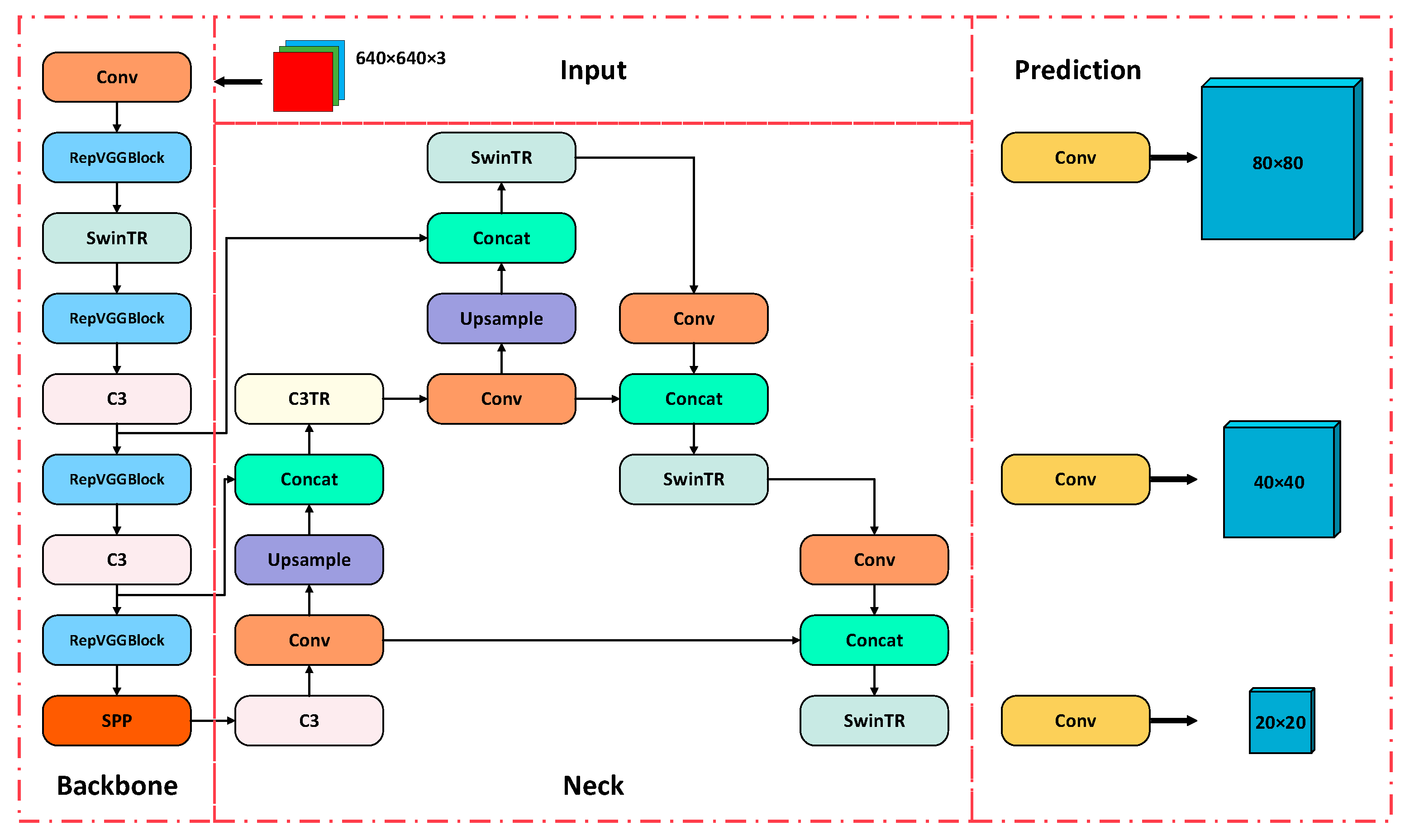
In the backbone of YOLOv5s, the SPP modules remain unchanged. The CBS module is replaced by the RepVGG module, i.e., the original network structure of YOLOv5s is replaced by the RepVGG lightweight network structure as the backbone network, which can effectively solve the gradient disappearance and gradient explosion problems of the model so that the overall detection accuracy and detection speed of the backbone network can be improved. The Swin Transformer module replaces the first layer C3 module and adds the self-attentive mechanism of a movable window, which can effectively capture global information and has the flexibility of multi-scale modeling. The first layer C3 module in the head of YOLOv5s remains unchanged, and the second layer C3 module is replaced by C3TR, which helps the convolutional network to filter the irrelevant information of the original image and promote the convergence of the network. The remaining C3 modules in the header are replaced with Swin Transformer modules, and the remaining modules are the same as those in the original YOLOv5s. Figure 8 depicts the structure of the improved network.

3.3. Improvement of SimOTA Based on YOLOv5s with Positive and Negative Sample Matching Strategy

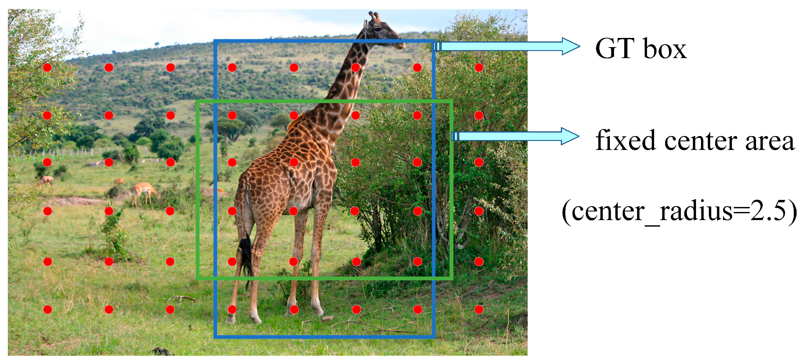
OTA (Optimal Transport Assignment) is a method of positive and negative sample matching strategy [44,45]; SimOTA is a simplification of it and can be seen as a problem of optimal assignment. SimOTA is considered to filter better positive samples to match the GT box (Ground Truth), thus reducing the cost.

First, a pre-screening of anchor points is required. In SimOTA, all the anchor points in the range of gt boxes are firstly boxed, and then a box of size 5 × 5 is set from the range of gt boxes, which is called the fixed center area, as depicted in Figure 9.

Calculate the cost function in the candidate region as follows equation.

$$\cos t_{ij}=L_{ij}^{cls}+\lambda L_{ij}^{reg}$$

(17)

where $L_{ij}^{cls}$ represents the classification loss, $L_{ij}^{reg}$ represents the positioning loss, and λ represents the balance coefficient of the positioning loss.

The classification loss (cls_loss) and position loss (iou_loss) for each anchor point with respect to each gt box are then calculated. First, we determine the ten lowest-cost feature points of each target. Next, we add up the IOUs of the prediction box and the real box corresponding to the ten feature points. The cost matrix and iou matrix are obtained based on the classification loss cls_loss and location loss iou_loss. The cost matrix is used to determine the dynamic_k anchor point with the lowest cost value for each gt box. The loss calculation is performed for the filtered prediction box, and the equation is:

$$Loss=(L_{cls}+\lambda L_{reg}+L_{obj})/N_{pos}$$

(18)

where $L_{obj}$ represents the obj loss and $N_{pos}$ represents the number of Anchor Points that are divided into positive samples.

In comparison to OTA, using SimOTA speeds up the model calculation reduces training time, and does away with extra optimization parameters. The possible positive sample regions are selected to determine whether they are within the region of the label, and the cost matrix is introduced to make it adaptive to find the real frame to which the current feature points are de-fitted, increasing the number of de-fitted real frames. Meanwhile, SimOTA outperforms SOTA ultralytics-YOLOv3 [21]. This further demonstrates the high detection accuracy of SimOTA. Applying it to YOLOv5s can improve the detection accuracy and detection speed of the network.

4. Wildlife Testing Experiments and Analysis of Results

For the above-mentioned improvement of the YOLOv5s model, this paper applies it to the wildlife dataset in this paper. By observing and comparing the experimental results, we will validate the effectiveness of the improvement points and will further analyze the experimental results as well as the detection effects.

4.1. Experiment Environment

The experimental software environment is the Linux operating system; Pytorch was used as the deep learning framework, as well as CUDA4.2, cuDNN8.2, and Python 3.7.0.

The hardware environment of the experiment is Intel(R) Core(TM) i7-10750H CPU@2.60 GHz(12 CPUs), ~2.6 GHz, NVIDIA TESLA V100 32 G with 2 TB storage resources.

4.2. Experimental Data Set

The majority of the real-world animal photographs in the realistic shooting collections utilized in the studies are taken from public datasets. Similar to the VOC2007 and COCO datasets, the images in this paper were obtained from websites with publicly available animal images, such as Google, but these images were not labeled with the animals in the images, so we first needed to manually label the animals in the collected images when pre-processing the images. The images collected in this paper have a brief description of the animals within the images, which ensures the accuracy and quality of the annotation of the dataset in this paper.

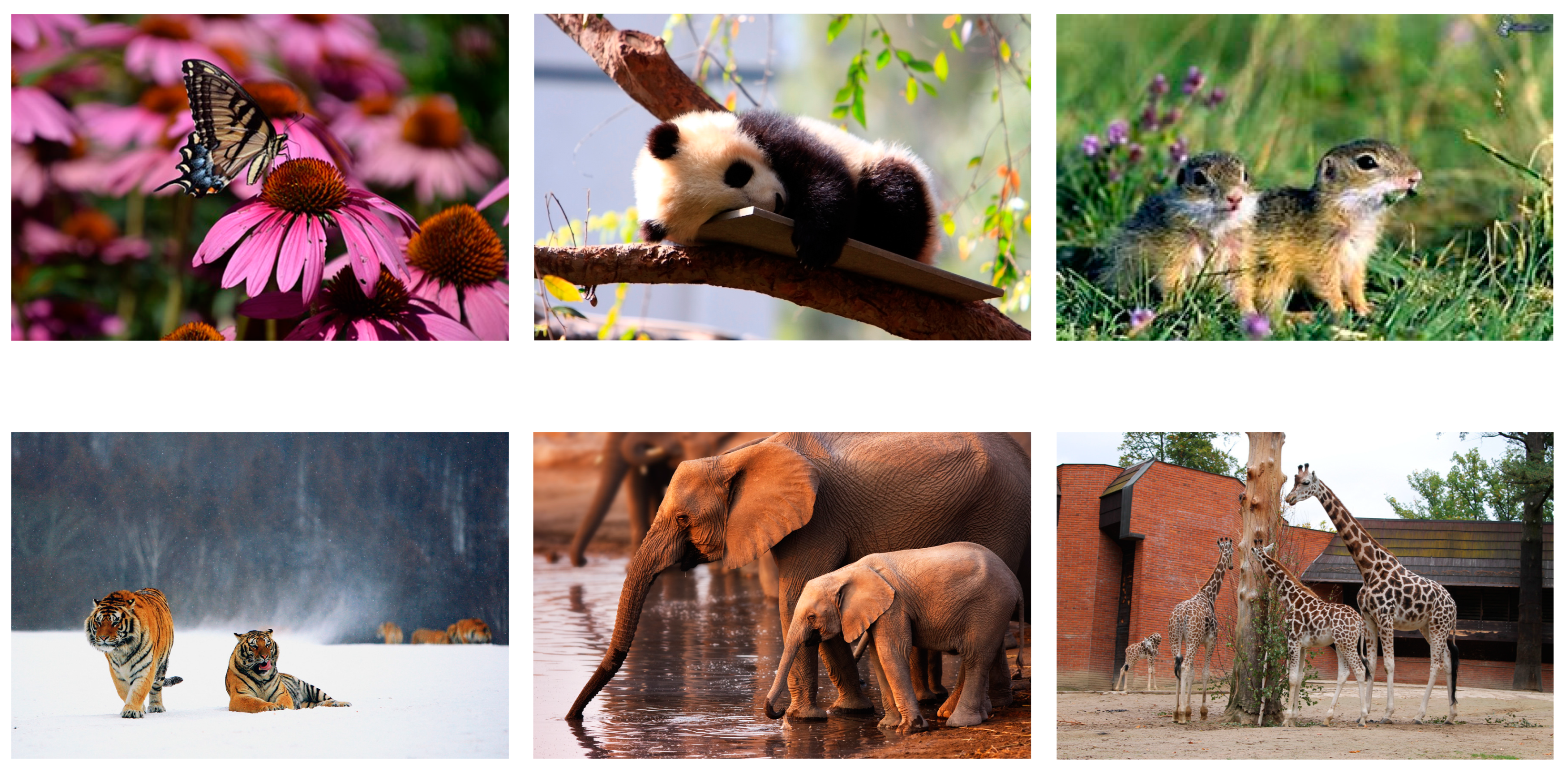
As seen in Figure 10, the dataset has Labelimg annotations in XML format. To better highlight the representativeness of the dataset in this paper, the example photos can be categorized into six groups based on the object classification of the dataset: panda, giraffe, elephant, tiger, butterfly, and squirrel. These animals live in Asia, Europe, and North America, and their living environments are representative of those of most animals, so the model can be extended to the detection and study of other animals, which greatly improves its environmental adaptability and generalizability.

There are 900 giraffes, 1100 butterflies, 1050 pandas, 1000 squirrels, 1000 tigers, and 1000 elephants. There are 6050 sample photos in total. The ratio is 6:2:2.

Table 1. Distribution of data sets.

Parameters	Number
Training sets	3630
Validation sets	1210
Test sets	1210
Total	6050

displays the produced dataset’s distribution.

Figure 11 displays sample images from the dataset for the animals used in this study.

4.3. Target Detection Experiments Based on Wildlife Dataset

After making the wildlife dataset, we converted the XML file into a TXT file and put it into the model for training. The experimental results were compared and analyzed. We trained the model in this paper using the training and validation sets that were split in the prior paper. To obtain the final experimental data, the model was tested after training using the previously divided test set.

GFLOPS (Giga Floating-point Operations Per Second), the number of billion floating-point operations per second, is usually used as a GPU performance parameter and can be observed by GFLOPs. The model’s parametric size, or parameters, can be used to determine how complex the model is by examining the parameters. In model improvement, sometimes GFLOPs and parameters inevitably increase. In general, we want the GFLOPs and parameters to be as small as possible.

Latency represents the inference time, and similarly, if each image takes t seconds to process, then the formula is Equation (19), and both parties can observe the model’s detection speed. FPS stands for the number of images identified per second. For the target detection model, the larger the FPS and the smaller the latency, the better the real-time performance of the model and the faster the computation speed of the model:

$$FPS=\frac{1}{t}$$

(19)

The precision rate is determined using Equation (20). It is defined as the ratio of the number of positive samples correctly predicted by the model to the total number of positive samples predicted:

$$precision=\frac{TP}{TP+FP}$$

(20)

The recall represents the number of positive samples correctly predicted by the model as a percentage of all targets. The formula for calculating the recall rate is shown in Equation (21):

$$recall=\frac{TP}{TP+FN}$$

(21)

The precision-recall curve is the curve shown with precision as the y-axis and recall as the x-axis. It is defined as the region enclosed by the axes below as average precision (AP). The accuracy values are displayed via the precision-recall curve when extra outer boxes are approved (i.e., higher recall values due to lower class probability thresholds). As the recall increases, a strong model can keep its precision high [37]. IoU (intersection over union) thresholds are typically set at 0.5. The performance of the model is generally better the higher the AP. For each type of animal detection, the higher the AP value, the better the detection of this type of animal, i.e., the higher the detection accuracy:

$$AP={\displaystyle {\int }_0^{1}P(R)dR}$$

(22)

As seen below, mAP (mean Average Precision) is the average accuracy across all species. For the whole model, the higher the mAP value, the better the overall detection effect of the model and the higher the detection accuracy:

$$mAP=\frac{1}{N}{\displaystyle \sum _{i=1}^{N}A{P}_i}$$

(23)

4.4. Experimental Results & Analysis

This research examines the target detection efficiency of the updated model on various types of animals before and after the improvement in order to analyze the usefulness of the improved algorithm on target detection for each animal.

Table 2. Experimental results of various types of wildlife testing before and after improvement.

Model	Butterfly	Panda	Squirrel	Tiger	Elephant	Giraffe
YOLOv5s	87.7	94.6	89.3	94.2	90.0	90.0
YOLOv5s_ours	91.3	94.1	95.5	95.6	94.2	94.6

presents the outcomes.

The experimental results demonstrated that the detection effect of all types of animals was improved. The detection accuracy was high when the wild animals themselves could be easily distinguished from the surroundings, and it was lower when the target detection model’s detection accuracy was more similar to that of the environment. The butterfly’s mAP in the original YOLOv5s algorithm is the lowest, at just 87.7%, and the panda’s mAP is the greatest, at 94.6%. The butterfly’s mAP in the upgraded YOLOv5s algorithm is the lowest, at just 91.3%, and the tiger’s mAP is the greatest, at 95.6%. The improved detection algorithm of YOLOv5s has improved the detection accuracy for large target animals, such as giraffes and elephants, due to the increased sensory field of the model, and the mAP for medium-sized animals, such as pandas and tigers can maintain the high detection accuracy before the improvement. There has been a major advancement in the identification of wild animals for some creatures, such as butterflies and squirrels, whose color patterns are protective or comparable to those of their natural habitat. This suggests that the enhanced YOLOv5s model presented in this study can more effectively carry out detection tasks for animals with a variety of sizes and morphologies in a variety of situations. For the improved YOLOv5s model, animals with different size targets and morphologies and animals with protective colors can have very good detection results, mainly attributed to the improvement of YOLOv5s network structure in expanding the sensory field.

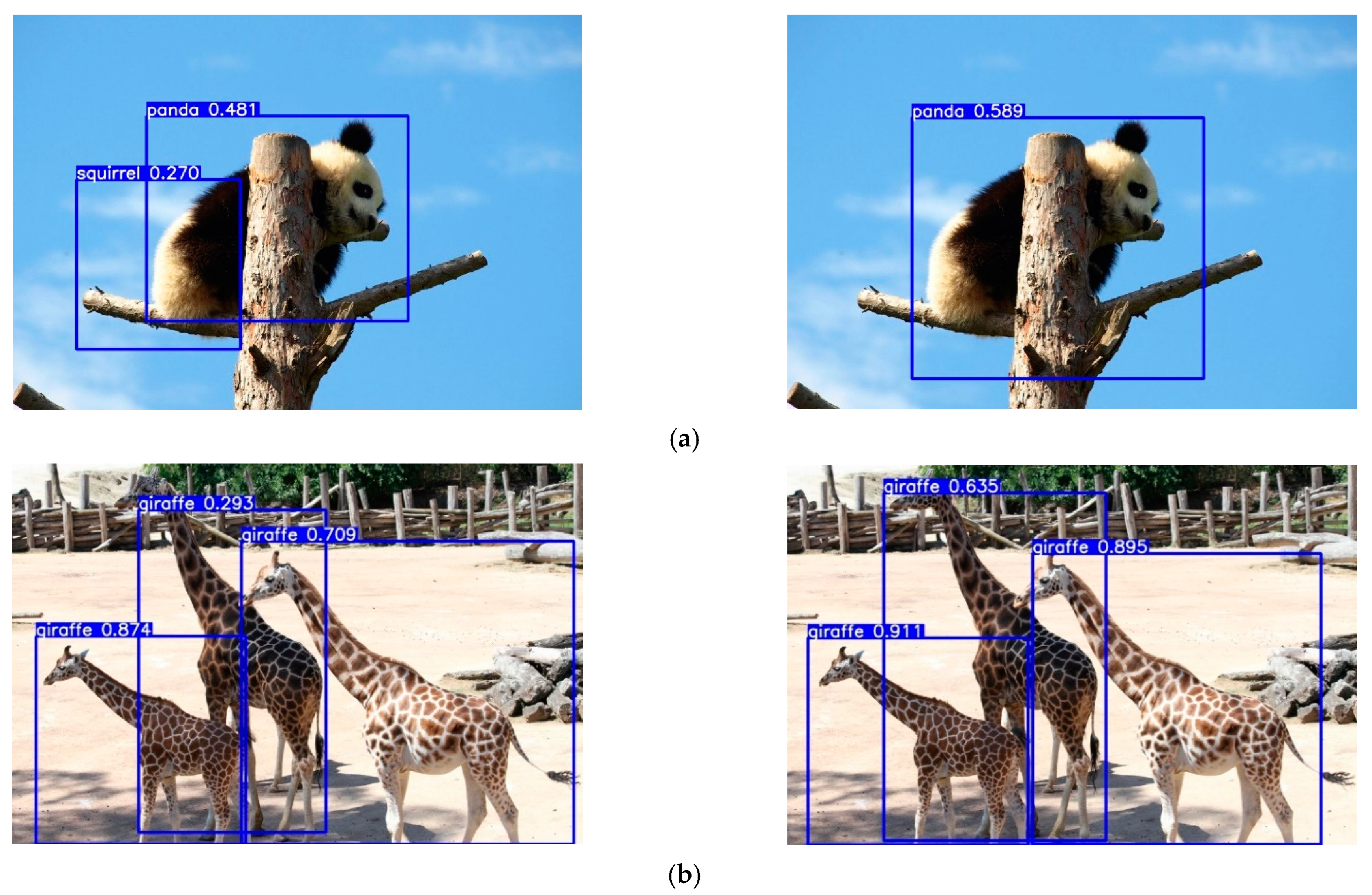
Four sample photographs were taken from the test set of the improved YOLOv5s model before and after for comparison. The results are given in Figure 12 to demonstrate the advantages of the enhanced YOLOv5s algorithm over the original YOLOv5s in this paper. The name of the identified target is listed in the detection box above it. The confidence level indicates how well the algorithm performed. The graphic shows that when compared to the original method, the improved YOLOv5s algorithm has a greater detection accuracy for photographs of animals.

The improved model does not accidentally misdetect the tree branches, and the improved YOLOv5s has a higher confidence level for panda detection, as can be seen from the comparison plots in Figure 12a. The original YOLOv5s model mistakenly detects the tree on the left as a panda when detecting the panda image because the tree branches overlap with the panda. The comparison graph in Figure 12b shows that the confidence level of the improved YOLOv5s model is significantly higher than the original YOLOv5s model for detecting giraffes when the three giraffes have overlapping bodies. The updated YOLOv5s model now has better feature extraction and feature fusion capabilities for wildlife photographs. It has good detection capacity in various natural environments, according to the examination of the above sample image detection results. In terms of detection and recognition, the enhanced YOLOv5s model performs better than the baseline model and dramatically lowers the rate of missed detection and erroneous detection of target animals.

Experiments on animal detection and ablation were carried out using both the initial YOLOv5s model and the enhanced YOLOv5s model. The improvement of the RepVGGBlock module, Swin Transformer, C3TR, and SimOTA is a component of the YOLOv5s target identification improvement approach provided in this research. The ablation experiments were carried out for each of the four improvement points, with the input image size being 640 × 640, to confirm the efficacy of these four improvement points. After classification and data statistics,

Table 3. Results of ablation experiments.

Model	RepVGG	SwinTR	C3TR	SimOTA	mAP	FPS	Latency
YOLOv5s	×	×	×	×	91.0	112.6	3.8
A	√	×	×	×	91.2	118.3	2.7
B	√	√	×	×	91.9	125.6	1.0
C	√	√	√	×	92.1	121.6	1.8
YOLOv5s_ours	√	√	√	√	94.2	124.5	1.4

displays the outcomes of the ablation trials.

The various perceptual fields collected from each branch are joined into an addable block when the RepVGGBlocks module has been included. The model’s feature extraction speed is then increased, the number of convolutional layers and model parameters are decreased, the original activation function ReLU is replaced with SiLU, and this network’s computational efficiency and detection accuracy are simultaneously increased. As can be observed from the table, mAP increases by 0.2%, FPS increases by 5.7, and latency drops by 28.95% when compared to the old model. Without reducing the perceptual field, the feature map is uniformly divided into four local windows. There is no information interaction between the windows, and each window is operated independently. As a result, the amount of operations becomes one-fourth of the original one, the speed of the model increases, the FPS improves by 7.3, and the latency decreases by 62.96%. At the same time, the mAP is improved by 0.7% because SW-MSA uses sliding windows to divide the feature map. In this way, some of the windows can receive information passed from multiple windows in the upper layer, which can reduce the loss of perceptual fields and thus improve the representational power and nonlinear expression of the model. C3TR module is the replacement of TransformerBlock with BottleNeck in the C3 module, which has a small perceptual field and weak feature extraction capability when performing target detection because the scale of targets within the image is mostly different. Based on this, C3TR divides the feature map into multiple and then takes the extracted feature information as input in the form of a one-dimensional vector, which improves the convergence ability of the model. At the same time, the model introduces a multi-headed self-attention mechanism and multi-layer perception, so the global-based self-attention calculation can expand the perceptual field of the feature map and has a very strong learning ability. Therefore, it can be obtained from Table 3 that the mAP is improved by 0.2% after adding C3TR.SimOTA introduces the cost matrix. In the model, pre-screening is performed first; the sample points need to fall into both GT and fixed center areas and the candidate frames whose center points on the feature map are inside GT must be found. Then, execute the SimOTA assignment strategy for these candidate frames, dynamically assign dynamic candidate frames to each GT, then calculate the cost matrix, and find the respective minimum Loss from the cost matrix. SimOTA obtains the best learning result with the smallest cost, and the mAP is improved by 2.1%, as shown in Table 3. SimOTA introduces the cost matrix to replace the Sinkhorn–Knopp Iteration optimization algorithm, which shortens the time required for model training, thus, the FPS is improved by 2.9, and the latency is reduced by 22.2%.

4.5. Algorithm Comparison Analysis

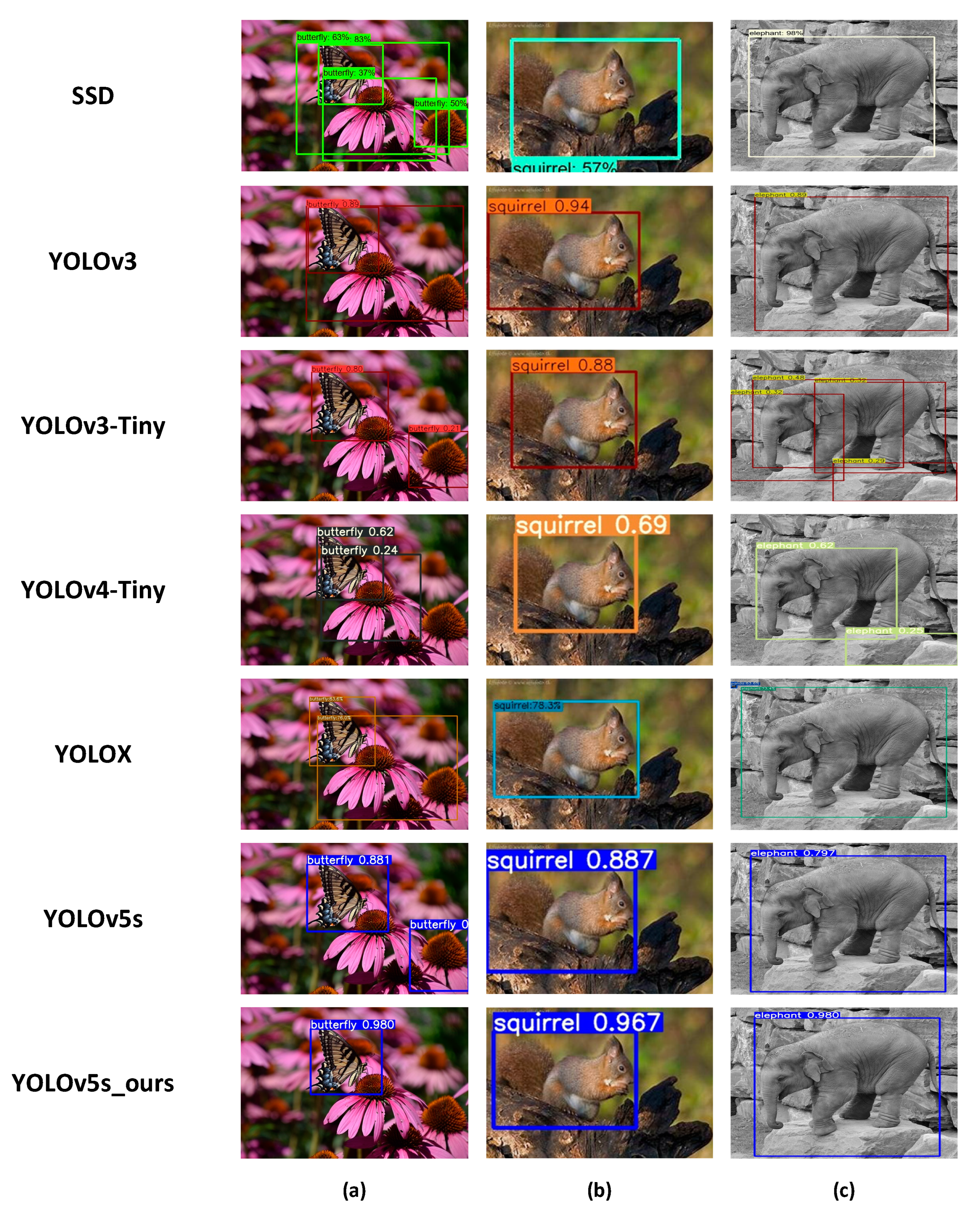
The data set from this paper was applied to SSD, and the YOLO series target detection algorithm for experiments, each of which was carried out independently. Among them, SSD uses VGG16 network structure, the YOLOX model is the YOLOX-S versions, YOLOv3, YOLOv3-tiny, YOLOv4-tiny, YOLOv5s are all Pytorch versions, and the models all run under the Pytorch framework. The obtained parameters, GFLOPs, mAP, and FPS, are shown in

Table 4. Performance comparison of target detection models.

Models	Size	Parameters/106	GFLOPs	mAP	FPS
SSD	300 × 300	99.8	31.0	0.779	69.1
YOLOv3	640 × 640	61.5	154.6	0.946	62.9
YOLOv3-tiny	640 × 640	8.69	12.9	0.853	94.7
YOLOv4-tiny	640 × 640	5.89	16.2	0.842	100.8
YOLOX	640 × 640	8.94	26.7	0.899	91.8
YOLOv5s	640 × 640	7.07	16.3	0.910	112.6
YOLOv5s_ours	640 × 640	7.25	33.7	0.942	124.5

to demonstrate that the improved YOLOv5s algorithm in this paper outperforms other target detection algorithms for wild animals in the natural environment. By comparing the final analysis, we can get that the performance of the improved YOLOv5s model is better than the other comparative algorithms.

In Table 4, we can see that the mAP and FPS of YOLOv3-tiny, YOLOv4-tiny, and YOLOv5s, which are close in size to the parameters and GFLOPs of YOLOv5s_ours, are all lower than those of YOLOv5s_ours, and although the mAP of YOLOv3 is higher than that of YOLOv5s_ours, its model parameters are too many, its computation is extremely large, and its FPS is lower than most other algorithms, which cannot meet the requirement of real-time. Therefore, considering the above aspects, the improved YOLOv5s in this paper is more capable of detecting wild animals in the natural environment compared with other algorithms. In this paper, four detection results are taken from each of the test sets of all models for comparison, and similar to the previous, the higher confidence level in the detection box indicates the better performance of the algorithm, as shown in Figure 13.

5. Conclusions

In order to utilize YOLOv5s more effectively to target the detection of wild animals in natural habitats, an improved technique is proposed in this research. The improved algorithm introduces the concept of structural reparameterization, uses the RepVGGBlock and Swin Transformer modules to simplify the network structure, and divides the feature map using a sliding window, cutting the operation time in half compared to the original model. This quickens the model’s convergence rate and enhances its real-time performance. In comparison to the original YOLOv5s algorithm, the updated YOLOv5s algorithm increases the mAP by 3.2% and the FPS by 11.9 while also increasing the detection accuracy and detection speed. It serves as a guide for the creation of later animal detecting systems. Given that some wild animals have the ability to mimic in their natural environment, in the next step, we will improve the RGB channel to improve the model’s ability to analyze color so that the model can better identify animals that can mimic. This paper proposes an improved YOLOv5s algorithm for better detection of animals in the natural environment. The detection of animals in the natural environment will make it possible to discover species that are already endangered in a certain area and focus on protecting the ecological environment in that area to achieve the harmonious development of humans and nature. The algorithm can also be deployed on edge devices and can be used for commercial purposes, such as developing zoo management software. Future research will therefore concentrate on further network structure optimization to enhance performance in this area.