Smartwatch In-Air Signature Time Sequence Three-Dimensional Static Restoration Classification Based on Multiple Convolutional Neural Networks

Abstract

In-air signatures are promising applications that have been investigated extensively in the past decades; an in-air signature involves gathering datasets through portable devices, such as smartwatches. During the signing process, individuals wear smartwatches on their wrists and sign their names in the air. The dataset we used in this study collected in-air signatures from 22 participants, resulting in a total of 440 smartwatch in-air signature signals. The dynamic time warping (DTW) algorithm was applied to verify the usability of the dataset. This paper analyzes and compares the performances of multiple convolutional neural networks (CNN) and the transformer using median-sized smartwatch in-air signatures. For the four CNN models, the in-air digital signature data were first transformed into visible three-dimensional static signatures. For the transformer, the nine-dimensional in-air signature signals were concatenated and downsampled to the desired length and then fed into the transformer for time sequence signal multi-classification. The performance of each model on the smartwatch in-air signature dataset was thoroughly tested with respect to 10 optimizers and different learning rates. The best testing performance score in our experiment was 99.8514% with ResNet by using the Adagrad optimizer under a $1\times {10}^{-4}$ learning rate.

1. Introduction

With the development of embedded sensors in various portable devices, in-air signature recognition has made a lot of progress in recent years [1]. The main ideology for in-air signature signing involves using external devices, such as mobile phones [2,3], smart watches [4], high-speed cameras [5,6], and leap motion controllers [7,8] to capture the digital signals of the in-air signatures and analyze the information to recognize the identities of individuals. The in-air signature has been studied a lot because it is traceless, contactless, and secure [9,10], showing great strength compared with the other identification methods. Given the advantages of the in-air signature, various time-series models, such as the transformer [11], RNN [12], and LSTM [4] have been applied to the in-air signature recognition. With the development of image recognition technologies, the convolutional neural network (CNN) has been evolving at a fast speed [13]. Nevertheless, there is rarely any research on the performance evaluations of the convolutional neural networks for median-sized in-air signature recognition; the main reason is that in-air signatures are time-series signals and CNN generally takes in the image information [8]. To address this problem, one of the novelties of our experiment involved using the three-dimensional restoration of the in-air signature converted from digital signals as the CNN model input. The results show that ResNet has the highest classification accuracy in the CNN model group at 99.8514% and other CNN models show consistent effective performance on median-sized in-air signature datasets while the transformer [11] is not suitable for median-sized in-air signature time sequence multi-classification tasks and shows over-fitting in different degrees over 50 repetitions. In our research, we used the smartwatch in-air signature dataset [4] consisting of 22 participants and 440 in-air signatures (with 220 being genuine and 220 being forgeries). The convolutional neural network models and the representative time sequence model, the transformer, were tested on the median-sized in-air signature dataset based on a smartwatch. We implemented the DTW algorithm [14] to verify the usability of the smartwatch dataset first, and from there, the experiment took two different branches. For convolutional neural network models, in-air signature signals were first converted to static 3D restorations as images; four CNN models, i.e., LeNet [15], AlexNet [16], VGG [17], and ResNet [18], were implemented and tested for the smartwatch in-air signature dataset. For the time sequence model, the smartwatch nine-dimensional in-air signature dataset goes through normalization, concatenation, and downsampling, and then the dataset is fed into the transformer for classification, which works as the baseline case for comparison. This paper is organized in the following manner. In the introduction section, the research procedure, experiment setup, and recent representative research on in-air signature recognition are discussed. In the materials and methods section, the dynamic time warping (DTW) algorithm is used to analyze the smartwatch in-air signatures. The proposal for the restoration of in-air signature section includes coverage of the system architecture, methodology for restoring in-air signatures, and a comparative study of CNN models. In the results section, we demonstrate the performance of ResNet together with the performance comparison of convolutional neural networks and the transformer with respect to different optimizers. In this section, the fine-tuned ResNet model is nominated and a comparison of different models is presented. Finally, we summarize our research and discuss the research limitations and future directions. To best replicate the experiment’s procedure, the computer configuration used in the research is listed in

Table 1. Computer configurations.

Computer Configurations
Item	Property
Processor	12th Gen Intel(R) Core(TM) i7-12700KF 3.61 GHz
Installed RAM	32.0 GB (31.8 GB usable)
System type	64-bit operating system, x64-based processor
GPU	NVIDIA GeForce RTX 3080

. One of the novelties of our experiment involves converting the time sequence in-air signature signals into a visible three-dimensional signature representation based on the in-air signature trajectory restoration. Finger movement trajectory restoration is widely used in medical studies for patients with amyotrophic lateral sclerosis (ALS) disease [19]. In research by Ziqian Xie et al. [20], electrocorticography (ECoG) signals were obtained to investigate neural reactions while patients conducted finger movements. Finger trajectory was learned using CNN [21] and LSTM [22] models. Similarly, in the study by Gert Pfurtscheller et al. [23], the neural reactions of patients during the movements could be observed based on EEG, which could be used as the database for training models. In our experiment, which is different from medical research fields using EEG, the in-air signature signals can be recorded by the accelerometer and gyroscope sensors embedded inside the smartwatch and the in-air signature trajectories can be restored based on the derivation of the acceleration signals (as covered later in the data processing section).

In the study by Jameel Malik et al. [5], the researchers proposed a new method called 3DAirSig, which mainly uses multidimensional dynamic time warping (MD-DTW); they collected 600 signature samples taken from the participants. Similar to the study by Guerra et al. [24], in this experiment, the 3D spatial signals of the signatures were taken into consideration. The signal analysis was in real-time, and a convolutional neural network was used to track the finger trajectories. The experiment shows an equal error rate (EER) of 0.46%. Hamed Ketabdar et al. designed the software called MagiSign [2] for the experiment. The software is based on the magnetic sensor embedded in the mobile phones and the participants can accomplish the signing registration process by using the magnet to draw their signatures around the mobile phone. Javier Guerra-Casanova et al. [25] collected in-air signatures from 50 participants to form an in-air signature dataset, and 6 participants mimicked the signing processing of the 50 participants to form a forgery dataset. The researchers used the DTW algorithm and LCS algorithm for the recognition, and the DTW algorithm outperformed the LCS, which gave 2.80% EER. In the study by Wee How Khoh et al. [26], the researchers collected signatures from 100 participants via a Microsoft Kinect sensor, and a self-designed algorithm was applied to the experiment to find the area of the palm location; the experiment used motion history image (MHI) to classify the in-air signatures from those participants and it achieved 90.4% accuracy. Shixuan et al. [27] investigated the effect of orientation on sensors and proposed an adaptive orientation method to learn and detect the pattern of data from different dimensions and process the sensor data separately based on each orientation. The ability and sensitivity of modern sensors to work as biometric confirmation have also been verified by Attaullah Buriro et al.’s research [28], in which multi-layer perceptrons (MLPs) were implemented to recognize the user’s identity through embedded sensors in portable devices. In the study by Abena Primo et al. [29], the effects of the spatial positions of portable devices were investigated through supervised learning, which helped improve the adaptability of in-air signatures in real applications. In the study by S.K. Behera et al. [8], the convolutional neural network was used to recognize the in-air signatures into the correct category. The researchers used the leap motion software to generate the trajectory of the in-air signatures. In the research, 700 signatures were collected for the classification. The experiment showed a 4% improvement in accuracy compared to the LSTM model and HMM. To fit the signals into the convolutional model, the signatures were first converted into one-dimensional data. Among all the techniques used in the in-air signature recognition field, S.K. Behera et al.’s approach [8] is the closest to our method. Instead of working on one-dimensional data, such as Behera et al., we used the restored signature images for the convolutional neural networks (CNNs). The comparative study in the CNN subsection will cover the CNN models we used for the experiment.

2. Materials and Methods

In-air signatures have made significant progress in the industry because of their contactless nature, which means that have an advantage over handwritten signatures. In the dataset that we used [4], 22 participants signed their names in the air using a smartwatch application. The technical characteristics are shown in

Table 2. The smartwatch technical characteristics used in the experiment.

Apple Watch Series 6 Configuration
Properties	Specifications
Chip	S6 SiP with 64-bit dual-core processor
	W3 (Apple wireless chip)
	U1 chip (Ultra Wideband)
Connectivity	LTE and UMTS
	GPS + Cellular models
	Wi-Fi 802.11b/g/n 2.4 GHz and 5 GHz
Sensor	Accelerometer (up to 32 g-forces with fall detection)
	Gyroscope

. During the signing process, participants wore the smartwatches on their wrists and finishes their signatures. Traditionally, the LSTM model [22], the transformer [11], and RNN [12] have been used for processing and recognizing the time series models. In our experiment, we compared the performances of the convolutional neural networks and transformer in terms of classifying in-air signatures. Moreover, we applied the DTW algorithm to verify the usability of the dataset. The experiment procedure is shown in Figure 1. We applied 10 different optimizers and learning rates to fine-tune the model to its best performance.

2.1. Data Acquisition

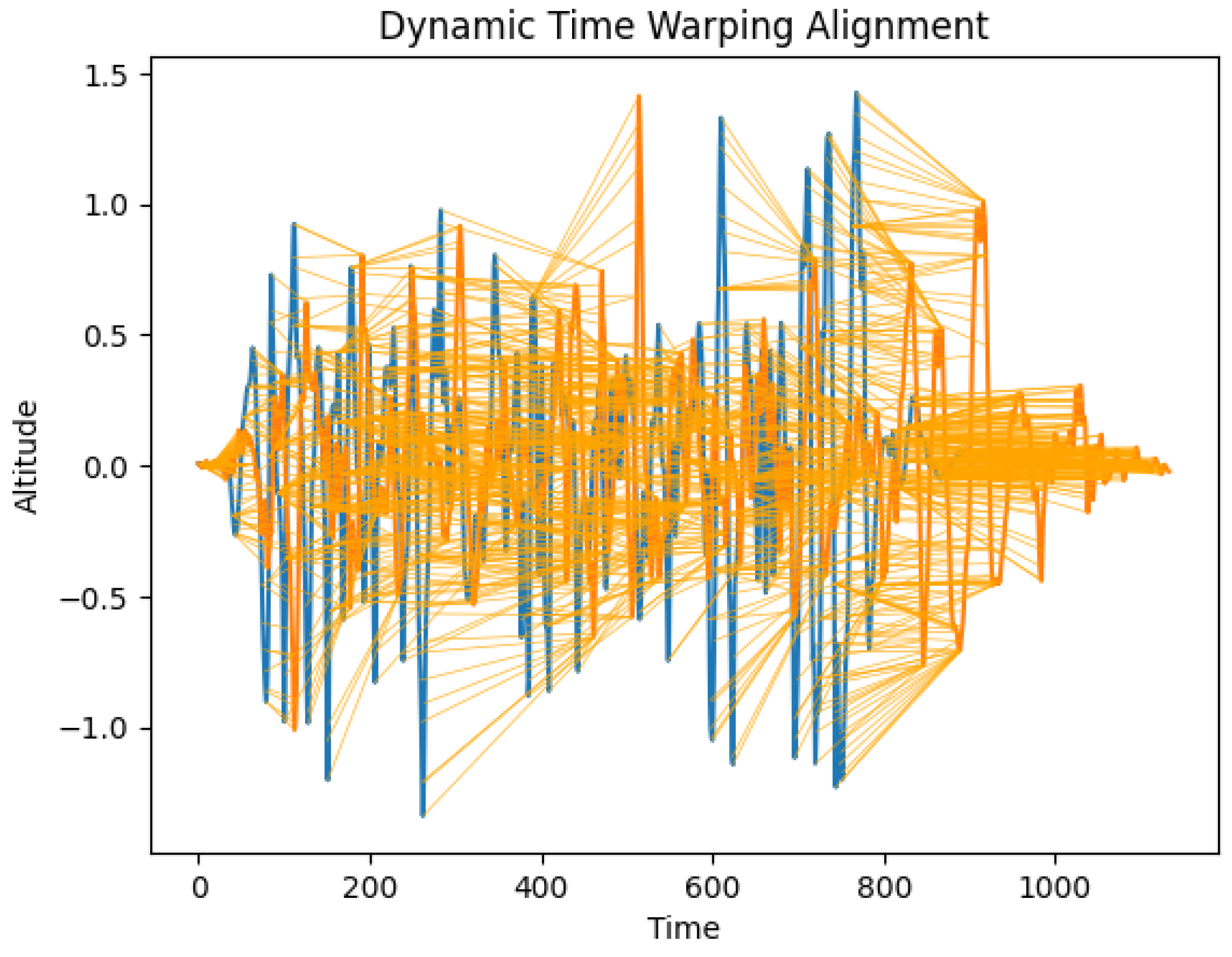
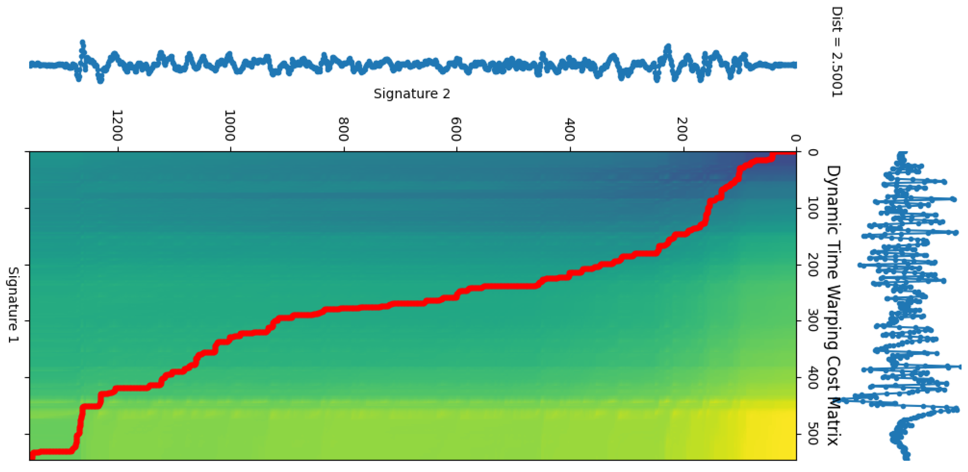
Given the various handwritten signature datasets listed by Mohammad Saleem et al. [30], a publicly available dataset for in-air signatures is rare. In our experiment, the dataset was conducted by Li [4] in his experiment on in-air signature biometrics based on the LSTM model. The smartwatch data formats are shown in

Table 3. Smartwatch in-air signature data format.

Smartwatch Data Format
WatchGyroX	WatchGyroY	WatchGyroZ	WatchAccX	WatchAccY	WatchAccZ	WatchAttX	WatchAttY	WatchAttZ
0.02570195	−0.03224608	−0.0120639	−0.01228451	−0.00830266	0.00186165	0.21137402	0.21104763	−0.75536253
0.02712557	−0.03940424	−0.0088675	−0.00624303	−0.00330171	0.00035724	0.2120575	0.21096044	−0.75540958
0.03478016	−0.0445323	−0.0054437	−0.00450777	0.00784102	−0.00614287	0.21283413	0.21098173	−0.75545861
0.05405451	−0.04379743	−0.01255126	−0.00808688	0.01724837	−0.0044408	0.21344206	0.21110055	−0.75555888
…	…	…	…	…	…	…	…	…

, which are part of the data gathered for one participant. For each participant, nine raw data features were collected from the accelerometer, gyroscope, and device attitude data based on the internal sensor embedded in the smartwatch.

2.2. Data Analysis

As shown in Figure 2, during the collection process of the smartwatch in-air signatures, all of the data gathered from the accelerometer and gyroscope were time-series signals; the three dimensions were x, y, and z-axis data. The time stamps are shown as deep blue to red colors, with blue representing an earlier time stamp and red representing a later time stamp. Figure 2 depicts the 10 genuine signatures of the same participant. The dynamic time warping algorithm (DTW) [14] can be used to verify the validity of the dataset. The DTW algorithm can detect distances among various time-series signals [6,31]. The distance measurement does not simply follow the Euclidean distance. The traditional Euclidean distance can only measure the static distance between two points while the DTW algorithm can be used to measure the distance of signals of different lengths. The DTW algorithm has many variations [32] and is widely applied to various time-series signal applications [33], including natural language processing [34].

$$c_p(X,Y):=\sum _{\ell =1}^{L}c\left(x_{n_{\ell }},y_{m_{\ell }}\right)$$

(1)

As shown in Algorithm 1 [35], the DTW [14] algorithm can create one-to-many alignments among two different signals as shown in Figure 3, in which the two signals are of different lengths. Those two accelerometer signals are samples taken from the same participant but of different categories, genuine signatures, and forgery signatures. The blue and the orange lines represent the fluctuations of two signals while the yellow line connecting the two signals is the alignment between the valley and peaks of two signatures.

Algorithm 1 Dynamic time warping [35]

Require: $u=\left\{u_1,u_2,\dots ,u_{T_u}\right\}$, $v=\left\{v_1,v_2,\dots ,v_{T_v}\right\}$     $g(0,0)=0$     $g(1,1)=d\left(u_1,v_1\right)·w_D$     for $iin[1\dots T_u]$ do           $g(i,0)=\infty$     end for     for $jin[1\dots T_v]$ do           $g(0,j)=\infty$     end for     for $iin[1\dots T_u]$ do           for $jin[1\dots T_v]$ do                 $g(i,j)=min(g(i,j-1)+d\left(u_i,v_j\right)·w_V,g(i-1,$                 $j-1)+d\left(u_i,v_j\right)·w_D,g(i-1,j)+d\left(u_i,v_j\right)·w_H)$           end for     end for     return $D(u,v)=k\left(w\right)·g\left(T_u,T_v\right)$                                        ▹ DTW-distance

The dynamic time warping cost matrix can be constructed as shown in Figure 4. The right and the top parts of the figure show the two in-air signatures; one of the signatures is from the genuine category of the participant while the other is from the forgery category of the participant. The dynamic time warping cost matrix shows the graduate changing from a dark blue color to a light yellow color; the dark blue color represents a lower alignment cost between the specific segments of the two matrices while the yellow color represents a high cost of alignment. Following the lower cost of the matrix, a warping path, shown as the red-colored line in the figure, goes from the origin to the last element of the matrix, and the total cost for the wrapping path can be calculated based on Formula (1) [36], in which $c_p$ represents the total cost while c represents the local cost. The last element of the matrix presents the accumulative alignment cost of the smartwatch’s in-air signatures, and the specific cost value is shown at the top-right corner of the figure.

Based on the DTW algorithm, for each participant, we can analyze the statistical correlations of the genuine and forgery categories based on the DTW distances. The DTW distance can be calculated based on Formula (2) [36], in which $p^{*}$ represents the optimal warping path. As shown in Figure 5, the genuine category and the forgery category of the same participant show a large distribution variance and this large variance applies to all 22 participants. Those large variances between different categories provide us with statistical support for using the convolutional neural network to classify the given signatures into the correct classifications.

$$\begin{array}{cc}\hfill DTW(X,Y)& :=c_{p^{*}}(X,Y)\hfill \\ \hfill & =min\{c_p(X,Y)\hfill \\ \hfill & \mid p\mathrm{is}\mathrm{an}(N,M)-\mathrm{warping}\mathrm{path}\}\hfill \end{array}$$

(2)

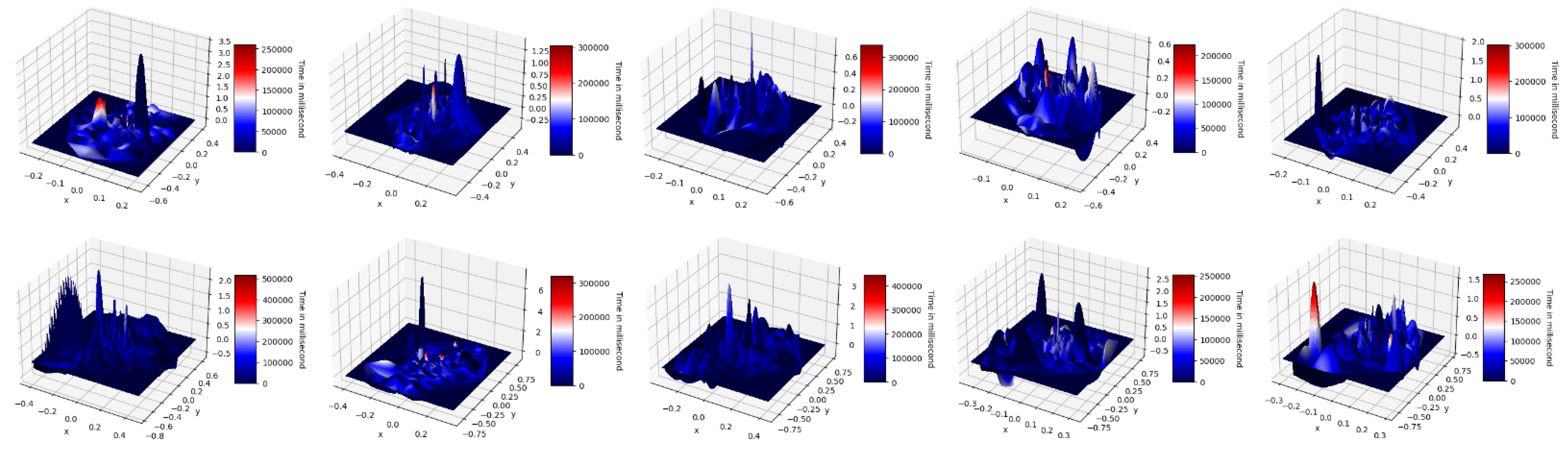
3. Proposal of Restoration of In-Air Signature

This section consists of three subsections. In Section 3.1, the details of the system architecture are discussed. In Section 3.2, the methodology of the in-air signature restoration is covered. In Section 3.3, the structure of the models used in our experiment is briefly introduced, including four CNN models (LeNet [15], AlexNet [16], VGG [17], and ResNet [18]) and a time sequence model (the transformer) [11], which works as the baseline for the CNN models.

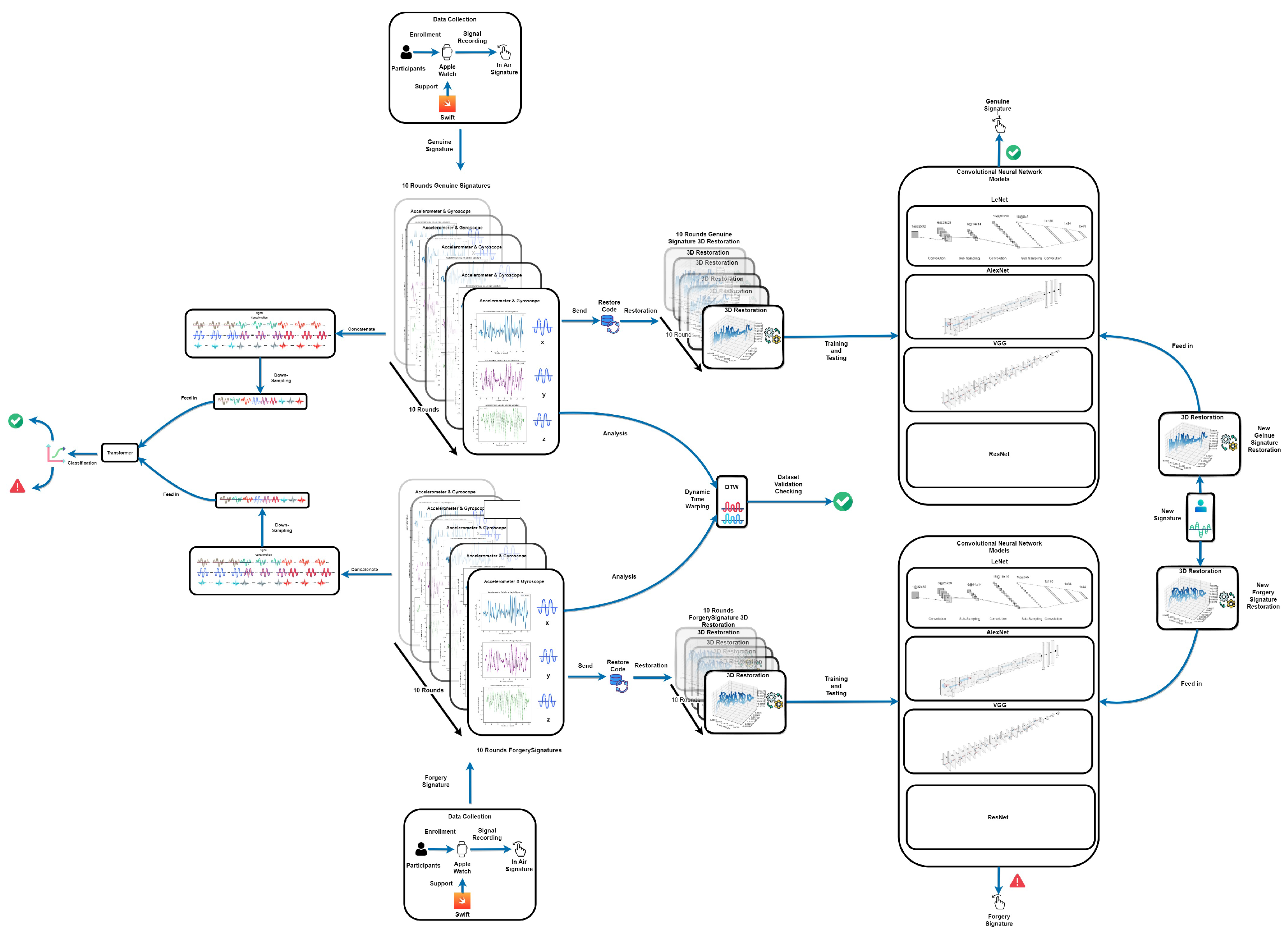
3.1. System Architecture

As shown in Figure 1 (note that some of the symbols in graphs are from Flaticon. The graph created was based on draw.io.), the system architecture of the experiment is illustrated in detail, including the structure of different convolutional neural networks. For each participant with the smartwatch worn on the wrist, the time-stamped in-air signature data information will be recorded based on the software developed through Swift [4,37]. With those in-air signature digital signals, we used the DTW algorithm [14] to verify the usability. After the data processing stage and restoration code, in-air signatures will be restored into visible three-dimensional in-air signature images. A transformation into desirable pixels will be conducted for different convolutional neural networks, respectively, as shown in Figure 6.

The real and forged in-air signatures after restoration will be labeled and marked into different classes. Subsequently, four different CNN models, including LeNet, AlexNet, VGG, and ResNet, are applied to the restored smartwatch in-air signature dataset. The structure of each convolutional neural network will be discussed in detail in Section 3.3, as shown in Figure 7, Figure 8 and Figure 9.

3.2. Methodology

One of the novelties of our experiment involved restoring the in-air signature into three-dimensional visible trajectories from the sensor embedded in the smartwatch, which can be used for classification using various convolutional neural networks. The accelerometer and the gyroscope sensors were embedded in the smartwatch generate acceleration signals in meters per square, and we tested the signature trajectory restoration based on the first derivative, the velocity signals, with respect to time, and the second derivative, the location signals, with respect to time. Even though the location signals, the second derivative, were supposed to give a better restoration of the trajectory by intuition, the noise was enlarged by a large degree, and the real meaningful location signals were overwhelmed by the noises. During the collection phase of the signature, noises were inevitably added to the signature signals. Nevertheless, the first deviation of the in-air signatures, velocity vectors, can best restore the in-air signature trajectories while minimizing the effects of the noises after testing.

In this way, the time series signals can be restored into visible signatures and this static reconstruction of signatures can also capture the time features. As shown in Figure 10, the area of the signature in a deeper blue represents a longer time spent in this area during the signing process. The three-dimensional in-air signatures were transformed into the desirable pixels for different CNN models as shown in Figure 6.

Unlike the traditional accelerometer-based in-air signature recognition, once the in-air signature restoration was constructed, using the more developed convolutional neural network could better solve the classification problem and improve recognition accuracy. Meanwhile, as a comparison baseline for convolutional models, the nine-dimensional time-series in-air signature digital signals were used directly after normalization, concatenation, and downsampling for the transformer. In our experiment, multiple optimizers were used for the fine-tuning purpose; these optimizers were Adadelta [38], Adagrad [39], Adam [40], AdamW [41], Adamax [40], ASGD [42], Ftrl [43], NAdam [44], RAdam [45], RMSprop [46], and SGD [47].

3.3. Comparative Study of CNN

LeNet [15] was one of the earliest proposed image recognition convolutional neural networks; it was first used for letter recognition. The LeNet structure, as shown in Figure 7, can be broken down into three fully linked layers, two sub-sampling layers, and two convolutional layers. (The LeNet concept is from [15] and the figure was created based on NN-SVG). One channel, six kernels, a stride of one, and a kernel size of five make up the first convolutional layer. Using a pool size of 2 and a stride of 2, we can construct the first pooling layer. The second convolutional layer has a stride of 1, 16 channels, 32 kernels, and a kernel size of 5. A pool size of 2 and a stride of 2 are likewise employed by the second pooling layer. The first fully connected layer, which follows the LeNet structure, is 32 × 5 × 5 to 120. The second fully linked layer is 120 to 84.

The AlexNet [16] model structure is illustrated in Figure 8. (The AlexNet concept is from the original paper [16] and the figure was created based on NN-SVG.) For the original AlexNet structure, two GPUs are used, and the top and bottom parts are identical structures. It mainly contains 5 convolutional layers and 3 max-pooling layers.

VGG [17] was first proposed in 2014, which illustrates 6 different structures of the VGG with subtle differences; the mostly used configuration is the D structure. Figure 9 shows the convolutional layer, max pooling layer, and fully connected layer, which give a better illustration of the structure. (The VGG concept is from the original paper [17] and the figure is finished based on NN-SVG). By substituting the large-size kernels with much smaller 3 by 3 kernels, which have the same receptive field, VGG can minimize the number of parameters [17]. We have 16 layers in the D architecture, comprising 3 fully connected layers and 13 convolutional layers. For the convolutional layers, the stride is 1 and the padding is 1. The max-pooling size and stride both equal 2. In a manner similar to AlexNet, we use 224 by 224 RGB input signature images, which are then passed into two 3 by 3 kernel layers with 64 kernels, max-pooling, two 3 by 3 kernel layers with 128 kernels, max-pooling, three 3 by 3 kernel layers with 256 kernels, max-pooling, three 3 by 3 kernel layers with 512 kernels, and a max-pooling layer. There are finally three fully connected layers.

ResNet [18], which employs extremely deep convolutional neural networks, was initially suggested in 2015. To address the degradation issue, it suggested using residual blocks, and to speed up training, it proposed using batch normalization rather than a dropout. The residual block sums up the input matrix through the shortcut together with the feature matrix following convolution before passing it into the ReLU activation function [48]. A much deeper convolutional neural network may be used without deterioration because of the residual block. For ResNet, batch normalization can be used to adjust the feature map distribution after the convolution, which satisfies the average to be zero and the variance to be one. The transformer [11] consists of multiple sets of encoders and decoders. Each of the encoders has the same structure but does not share the same parameters. For the encoder, it consists of input embedding, multi-head attention, and a feed-forward network. For the decoder, it consists of masked multi-head attention, multi-head attention, and a feed-forward network. In our experiment, the performance of the transformer is mainly used as the baseline reference for the rest of the convolutional neural network models.

4. Results

In this section, we first present the result of the four convolutional neural networks with respect to various learning rates and optimizers. Then the performance of the transformer is demonstrated as the baseline comparison. In the end, we discuss the performance comparison of the CNN and transformer and the best-fine-tuned result in our experiment.

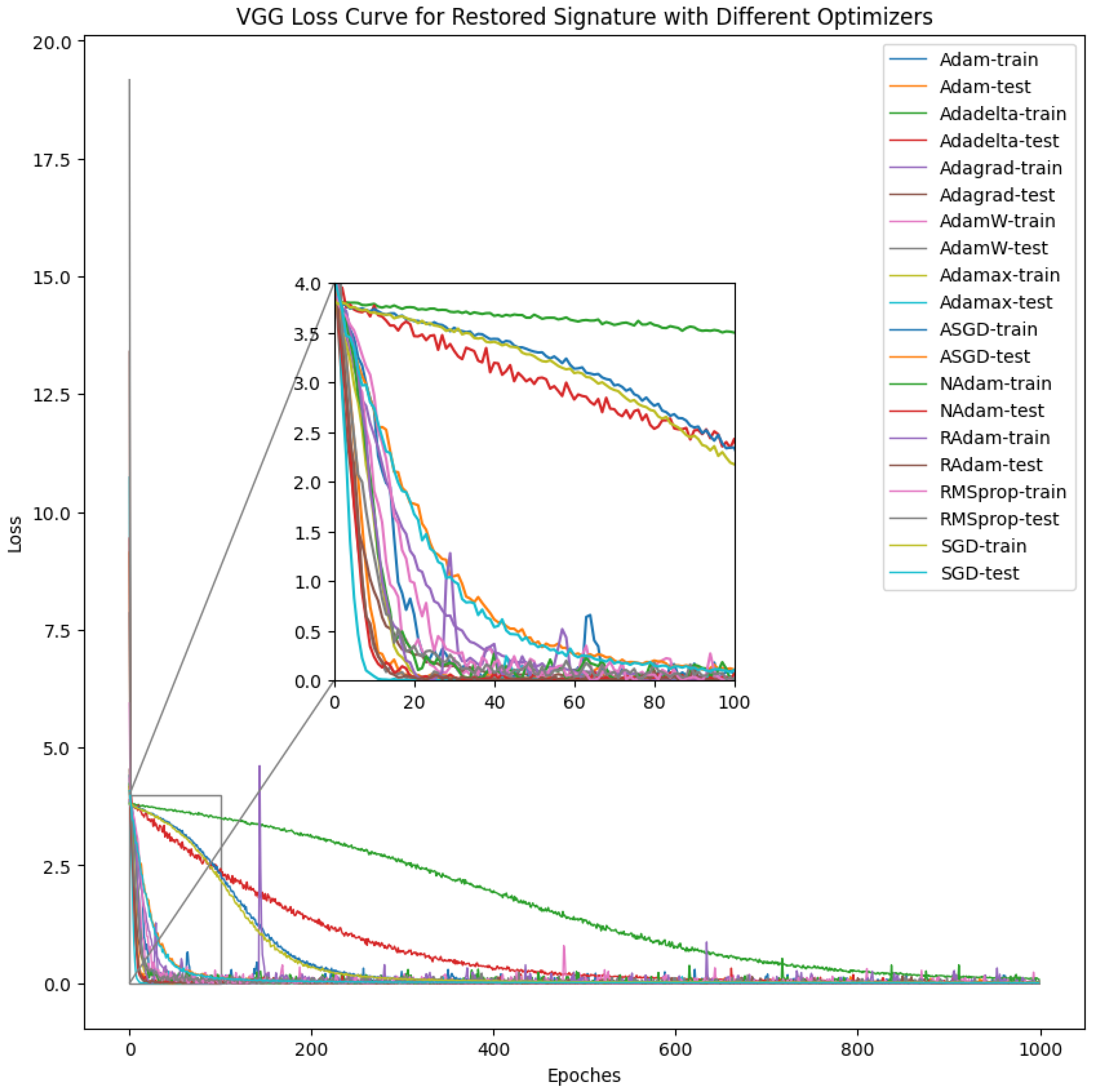
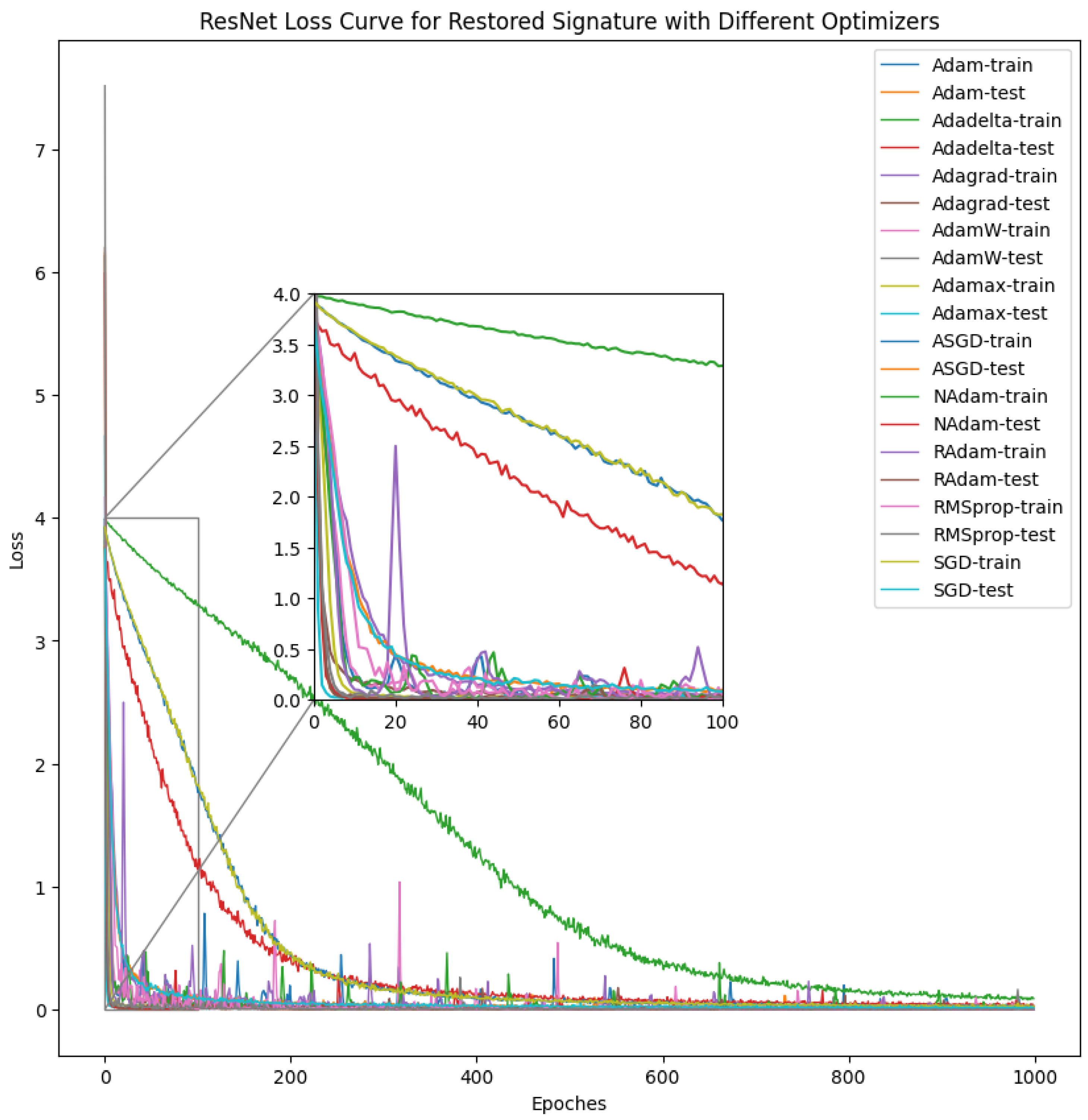
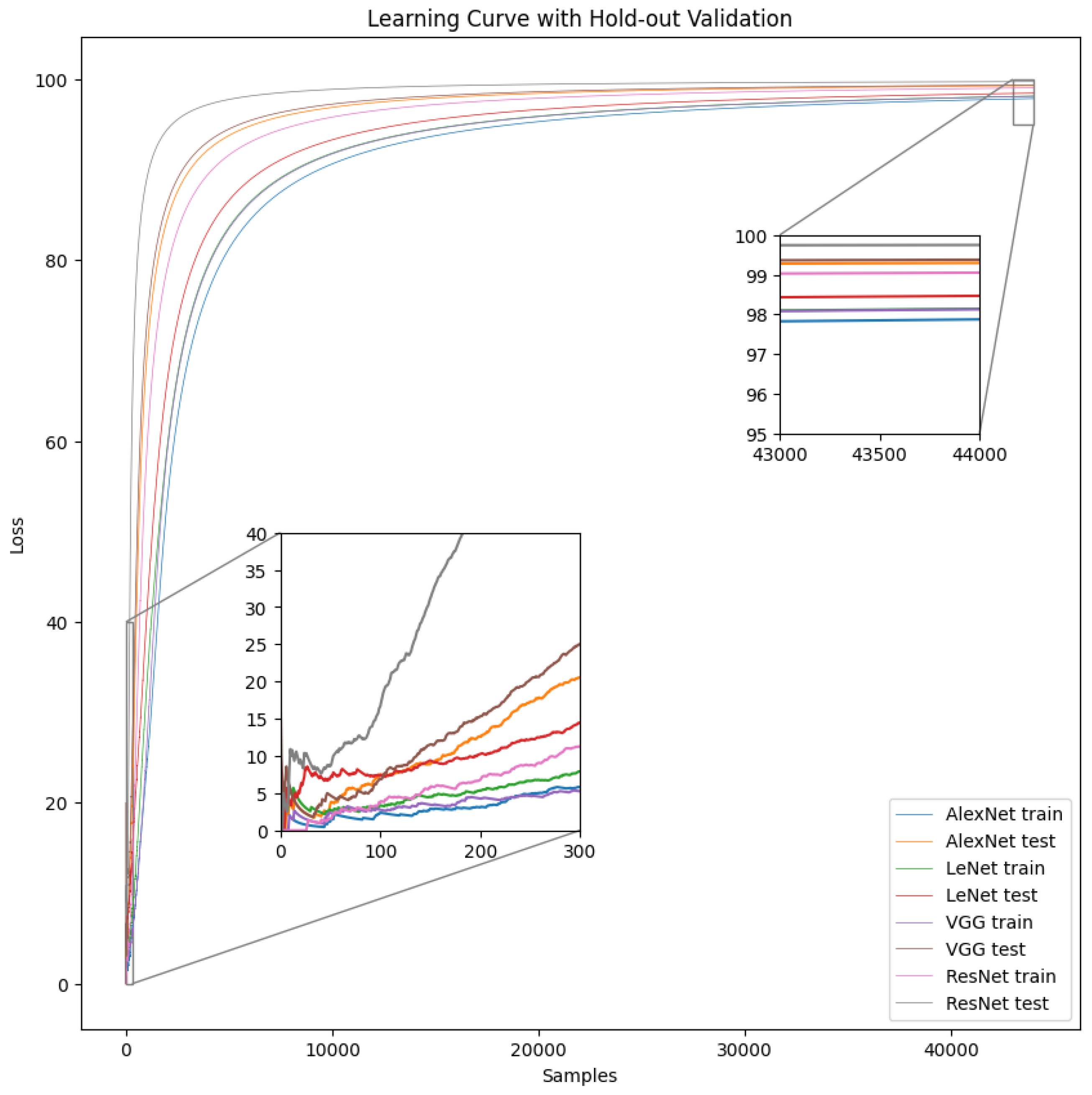
4.1. Convolutional Neural Network (CNN) Result

As a preliminary experiment, we tested the multi-class classification on the LeNet first. The mean and standard deviations were calculated for the image set. The restored signature was first transformed to the necessary pixel size and gray-scale pictures as seen in Figure 6 because LeNet [15] only accepts 32 by 32 one-channel gray-scale images. We had 22 participants and 44 categories; thus, the final fully connected layer was 84 to 44, as shown in Figure 7. For training and testing, the model employed cross-entropy loss and ReLU activation functions [48].

For AlexNet [16], similar to the LeNet, the mean, and standard deviations were calculated for the signature image set. However, AlexNet took in three-channel images, so the mean and standard deviations are in a list format, which is [0.88680416, 0.9199834, 0.95062685] for the mean and [0.22626287, 0.16366783, 0.103204496] for the standard deviations. Different from LeNet, AlexNet took in three-channel colored images of 224 by 224 pixels as shown in Figure 6. The model used in this experiment is identical to the original structure, except for the last output layer. The original paper had 1000 categories, it changed to 44 to fit the smartwatch in-air signature dataset.

The VGG [17] structure was modified from 1000 for the last fully connected layer that was initially used for ImageNet [49], which contained 1000 classes and 44 classifications. The size of the input did not change as it traveled through the convolutional layer but it was cut in half by the max-pooling layer since the max-pooling size was two and the stride size is two.

To better fine-tune the model, here are the results for each model with respect to the learning rate. The cross-entropy loss and stochastic gradient descent (SGD) [47] were chosen for each model, and we ran 1000 epochs for each model. For each epoch, the batch size was selected to be 5 to best minimize the loss oscillation. Given the dataset is relatively small, the model used hold-out validation with 50% for training and 50% for testing to reduce the possible bias in the testing process. As shown in

Table 4. All of the models use cross-entropy for the loss and stochastic gradient descent (SDG) for the optimizer. The bold value for the test score represents the best learning rate for performance. All of the loss values are in scientific notation while the scores are in percentage values, where “Inf” represent a very large loss value.

Model Performance with Respect to Learning Rate
Cross-Entropy & SDG		Learning Rate
Model	Criteria	$lr=1\times {10}^{-1}$	$lr=1\times {10}^{-2}$	$lr=1\times {10}^{-3}$	$lr=1\times {10}^{-4}$
LeNet	Train Loss	$2.78\times {10}^{-5}$	$2.32\times {10}^{-4}$	$2.15\times {10}^{-3}$	$3.52\times {10}^0$
	Train Score (%)	98.5995	98.0359	87.6746	24.3396
	Test Loss	$8.94\times {10}^{-6}$	$1.91\times {10}^{-4}$	$2.15\times {10}^{-3}$	$1.86\times {10}^0$
	Test Score (%)	99.4086	99.0645	98.8136	46.2164
AlexNet	Train Loss	Inf	$9.71\times {10}^{-1}$	$3.02\times {10}^{-3}$	$9.13\times {10}^{-3}$
	Train Score (%)	2.2718	84.3845	98.1127	97.8732
	Test Loss	Inf	$1.69\times {10}^0$	$3.04\times {10}^{-3}$	$6.04\times {10}^{-3}$
	Test Score (%)	2.2727	81.7914	97.6605	99.2946
VGG	Train Loss	Inf	$1.70\times {10}^{-3}$	$7.83\times {10}^{-3}$	$8.05\times {10}^{-3}$
	Train Score (%)	2.2727	87.4872	98.7905	98.1264
	Test Loss	Inf	$2.56\times {10}^{-2}$	$6.85\times {10}^{-3}$	$2.74\times {10}^{-3}$
	Test Score (%)	2.2727	93.5286	98.1041	99.3759
ResNet	Train Loss	$3.95\times {10}^{-1}$	$2.14\times {10}^{-2}$	$7.55\times {10}^{-4}$	$1.13\times {10}^{-3}$
	Train Score (%)	84.8318	96.0959	99.4000	98.9268
	Test Loss	$3.14\times {10}^{-1}$	$1.08\times {10}^{-2}$	$7.47\times {10}^{-3}$	$7.79\times {10}^{-4}$
	Test Score (%)	83.6241	98.9127	99.4386	99.7723
Transformer (Baseline)	Train Loss	$3.78\times {10}^0$	$2.69\times {10}^{-1}$	$2.27\times {10}^0$	$3.47\times {10}^0$
	Train Score (%)	0.0356	0.9609	0.5872	0.1103
	Test Loss	$3.86\times {10}^0$	$5.27\times {10}^0$	$3.78\times {10}^0$	$3.93\times {10}^0$
	Test Score (%)	0.0000	0.0282	0.0704	0.0423

, to evaluate the effect of the learning rate on the model and dataset, we kept the loss function fixed to cross-entropy loss and the optimizer fixed to be stochastic gradient descent (SGD); the bold numbers show the highest testing score for each of the learning rates with the corresponding model. The highest testing score was 99.77% for ResNet with a learning rate of $1\times {10}^{-4}$, which is reasonable because ResNet uses a much deeper network and batch normalization to adjust the distribution of the feature map. Additionally, the best testing scores for AlexNet and VGG all exist in the $1\times {10}^{-4}$ learning rate field. Leslie N. Smith’s research [50] also supports that for a relatively small dataset, choosing a lower learning rate can be more suitable for the model. The accuracy is expected to be lower if we expand our dataset, which is also one of the problems in this proposed recognition method if we want to apply the technique to industries. If more users are registered into the recognition system, and more classification categories are needed to be created, it may result in an unbalanced dataset with lower accuracy [51].

With the learning rate fixed to $1\times {10}^{-4}$ and the loss function fixed to cross-entropy loss,

Table 5. All of the models used cross-entropy loss and kept the learning rate fixed at $1\times {10}^{-4}$. The performance of each model (with respect to 10 different optimizers) was tested to fine-tune the performance within 1000 epochs. All of the loss values are in scientific notation while the scores are in percentage values. Please note that for the ASGD/Ftrl column, the Ftrl optimizer [43] was solely used for the transformer as ASGD [42] is not supported by Keras [52]. ASGD was used for the rest of the optimizers in the ASGD/Ftrl column, as it is supported by PyTorch [53].

Model Performance with Respect to Optimizers
$lr=1\times {10}^{-4}$ & Cross-Entropy		Optimizers
Model	Criteria	Adadelta	Adagrad	Adam	AdamW	Adamax	ASGD/Ftrl	NAdam	RAdam	RMSprop	SGD
LeNet	Train Loss	$3.71\times {10}^0$	$3.57\times {10}^0$	$7.15\times {10}^{-8}$	$1.65\times {10}^{-6}$	$0.00\times {10}^0$	$3.33\times {10}^0$	$1.91\times {10}^{-7}$	$0.00\times {10}^0$	$0.00\times {10}^0$	$3.52\times {10}^0$
	Train Score (%)	5.0468	28.7778	98.1396	97.9845	93.0550	12.0159	98.0236	97.0636	97.9309	24.3396
	Test Loss	$3.69\times {10}^0$	$3.32\times {10}^0$	$8.01\times {10}^{-6}$	$4.26\times {10}^{-5}$	$1.91\times {10}^{-7}$	$2.38\times {10}^0$	$1.53\times {10}^{-5}$	$2.15\times {10}^{-7}$	$4.08\times {10}^{-5}$	$1.86\times {10}^0$
	Test Score (%)	3.8445	12.1927	98.4664	98.4068	92.9855	34.8241	98.1705	98.4814	96.4250	46.2164
AlexNet	Train Loss	$1.31\times {10}^0$	$2.13\times {10}^{-3}$	$0.00\times {10}^0$	$0.00E\times {10}^0$	$0.00\times {10}^0$	$2.22\times {10}^{-2}$	$0.00\times {10}^0$	$0.00\times {10}^0$	$3.89\times {10}^{-2}$	$9.13\times {10}^{-3}$
	Train Score (%)	55.5791	98.0123	97.7586	97.7295	98.8518	89.1786	97.8955	97.4246	97.4186	97.8732
	Test Loss	$2.51\times {10}^{-1}$	$6.72\times {10}^{-3}$	$0.00\times {10}^0$	$0.00\times {10}^0$	$1.67\times {10}^{-7}$	$4.10\times {10}^{-3}$	$0.00\times {10}^0$	$0.00\times {10}^0$	$0.00\times {10}^0$	$6.04\times {10}^{-3}$
	Test Score (%)	70.4927	98.2100	98.5827	98.7150	99.4232	97.4268	98.5796	98.5955	98.1386	99.2946
VGG	Train Loss	$1.51\times {10}^{-1}$	$1.00\times {10}^{-3}$	$0.00\times {10}^0$	$8.13\times {10}^{-6}$	$0.00\times {10}^0$	$7.09\times {10}^{-3}$	$0.00\times {10}^0$	$0.00\times {10}^0$	$7.67\times {10}^{-1}$	$8.05\times {10}^{-3}$
	Train Score (%)	81.4840	98.8759	97.8546	98.1414	99.0646	94.1918	98.2309	97.9536	97.8327	98.1264
	Test Loss	$6.63\times {10}^{-2}$	$1.03\times {10}^{-3}$	$0.00\times {10}^0$	$0.00\times {10}^0$	$0.00\times {10}^0$	$2.29\times {10}^{-3}$	$0.00\times {10}^0$	$0.00\times {10}^0$	$7.87\times {10}^{-7}$	$2.74\times {10}^{-3}$
	Test Score (%)	88.2750	99.4282	99.0191	99.1255	99.5205	98.3523	99.1636	99.1818	98.4050	99.3759
ResNet	Train Loss	$5.95\times {10}^{-2}$	$4.29\times {10}^{-3}$	$2.02\times {10}^{-4}$	$4.41\times {10}^{-6}$	$2.96\times {10}^{-6}$	$5.41\times {10}^{-2}$	$1.32\times {10}^{-5}$	$7.04\times {10}^{-5}$	$3.10\times {10}^{-7}$	$1.13\times {10}^{-3}$
	Train Score (%)	85.6623	99.6332	99.1150	99.0900	99.7636	97.6668	99.1091	98.9477	99.0100	98.9268
	Test Loss	$1.73\times {10}^{-2}$	$3.11\times {10}^{-3}$	$4.03\times {10}^{-5}$	$1.44\times {10}^{-5}$	$3.57\times {10}^{-5}$	$3.42\times {10}^{-2}$	$2.72\times {10}^{-6}$	$4.10\times {10}^{-4}$	$3.45\times {10}^{-5}$	$7.79\times {10}^{-4}$
	Test Score (%)	96.3550	99.8514	99.6814	99.6777	99.8427	99.5318	99.6905	99.6505	99.6600	99.7723
Transformer (Baseline)	Train Loss	$3.73\times {10}^0$	$5.77\times {10}^{-1}$	$3.77\times {10}^0$	$3.78\times {10}^0$	$1.04\times {10}^0$	$1.30\times {10}^0$	$3.31\times {10}^0$	$1.12\times {10}^0$	$1.24\times {10}^1$	$2.69\times {10}^{-1}$
	Train Score (%)	0.0463	0.9288	0.0356	0.0249	0.8683	0.7331	0.6228	0.7758	0.5089	0.9609
	Test Loss	$3.97\times {10}^0$	$4.20\times {10}^0$	$3.89\times {10}^0$	$3.84\times {10}^0$	$4.37\times {10}^0$	$3.88\times {10}^0$	$1.24\times {10}^1$	$1.19\times {10}^1$	$1.94\times {10}^1$	$5.27\times {10}^0$
	Test Score (%)	0.0000	0.08451	0.0000	0.0000	0.1268	0.1127	0.0704	0.0563	0.0704	0.0282

shows the model performance with respect to different optimizers, in which 10 optimizers are tested for the performance. We ran 1000 epochs for each optimizer and a batch size of 5 to best evaluate the optimizer performance. As shown in Table 5, the training loss, train score, test loss, and test score were evaluated with respect to the optimizers. The 10 optimizers covered in the experiment were Adadelta [38], Adagrad [39], Adam [40], AdamW [41], Adamax [40], ASGD [42], NAdam [44], RAdam [45], RMSprop [46], and SGD [47].

LeNet, as an old-fashioned convolutional neural network, shows a slightly worse performance compared with other models. Figure 11 shows the loss curve for LeNet with respect to each of the optimizers. The largest train loss optimizer for the LeNet is Adagrad with a value of $3.57\times {10}^0$; the smallest train loss optimizers for the LeNet are Adamax, RAdam, and RMSprop, with a value of $0.00\times {10}^0$. The largest test loss optimizer for the LeNet is Adagrad with a value of $3.69\times {10}^0$ and the smallest train loss optimizer for the LeNet is Adamax with a value of $1.91\times {10}^{-7}$. The best train score optimizer for LeNet is Adam, with a score of 98.1396% and the worst train score optimizer for LeNet is Adadelta, with a score of 5.0468%. The best test score optimizer for LeNet is RAdam, with a score of 98.4814% and the worst test score optimizer for LeNet is Adadelta, with a score of 3.8445%. The results show that the RAdam optimizer has a better performance in combination with the LeNet, which can be supported by the study by Ke Cui et al. [54]. In their experiment, the combination of the RAdam optimizer and LeNet was chosen for currency recognition through transfer learning, in which the accuracy improved from 95% to 99.97%.

As a traditional CNN, AlexNet is one of the most powerful networks in the field of conventional convolutional neural networks. Figure 12 shows the loss curve for AlexNet with respect to each of the optimizers. The largest train loss optimizer for the AlexNet is Adadelta with a value of $1.31\times {10}^0$ and the smallest train loss optimizers for AlexNet are Adam, AdamW, Adamax, NAdam, and RAdam, with a value of $0.00\times {10}^0$. The largest test loss optimizer for AlexNet is Adadelta, with a value of $2.51\times {10}^{-1}$, and the smallest train loss optimizers for the AlexNet are Adam, AdamW, NAdam, RAdam, and RMSprop, with a value of $0.00\times {10}^0$. The best train score optimizer for AlexNet is Adamax, with a score of 98.8518% and the worst train score optimizer for AlexNet is Adadelta, with a score of 55.5791%. The best test score optimizer for AlexNet is Adamax, with a score of 99.4232%, and the worst test score optimizer for AlexNet is Adadelta, with a score of 70.4927%. The superior performance of the combination of AlexNet and Adamax can be supported by the study conducted by N. A. M. Ariff et al. [55]. The study compares the performance of AlexNet with the assistance of Adam and Adamax on 20 audio files. In this experiment, the combination of AlexNet and Adamax shows a greater performance than the normal Adam optimizer.

VGG serves as the foundation for modern convolutional neural networks and has shown excellent performance in our in-air signature dataset. Figure 13 shows the loss curve for VGG with respect to each of the optimizers. The largest train loss optimizer for the VGG is Adadelta with a value of $1.51\times {10}^{-1}$, and the smallest train loss optimizers for the VGG are Adam, Adamax, NAdam, and RAdam, with a value of $0.00\times {10}^0$. The largest test loss optimizer for the VGG is Adadelta, with a value of $6.63\times {10}^{-2}$, and the smallest train loss optimizers for the VGG are Adam, AdamW, Adamax, NAdam, and RAdam, with a value of $0.00\times {10}^0$. The best train score optimizer for VGG is Adamax, with a score of 99.0646% and the worst train score optimizer for VGG is Adadelta, with a score of 81.4840%. The best test score optimizer for VGG is Adamax, with a score of 99.5205%, and the worst test score optimizer for VGG is Adadelta, with a score of 88.2750%. The combination of the VGG and Adamax for image classification is popular in research; for example, in the medical study by Lorencin Ivan et al. [56], the VGG-16 structure is used for bladder cancer diagnosis. The combination of VGG-16 and the Adamax optimizer can successfully detect bladder cancer images with an accuracy of 0.98.

ResNet is one of the most powerful convolutional neural networks in the decades and it works as the foundation for variations of modern CNNs. Figure 14 shows the loss curve for ResNet with respect to each of the optimizers. The largest train loss optimizer for the ResNet is ASGD, with a value of $5.41\times {10}^{-2}$, and the smallest train loss optimizer for the ResNet is RMSprop, with a value of $3.10\times {10}^{-7}$. The largest test loss optimizer for the ResNet is ASGD, with a value of $3.42\times {10}^{-2}$, and the smallest train loss optimizer for the ResNet is NAdam, with a value of $2.72\times {10}^{-6}$. The best train score optimizer for ResNet is Adamax, with a score of 99.7636%, and the worst train score optimizer for ResNet is Adadelta, with a score of 85.6623%. The best test score optimizer for ResNet is Adagrad, with a score of 99.8514%, and the worst test score optimizer for ResNet is Adadelta, with a score of 96.3550%. In the study by Yang Jie et al. [57], the comparison between different CNN structures in combination with various optimizers was conducted for weed detection, in which the combination of the ResNet and Adagrad outperformed other optimizers with an accuracy of 0.98. The research can be used as statistical support for the performance of the ResNet and Adagrad combination.

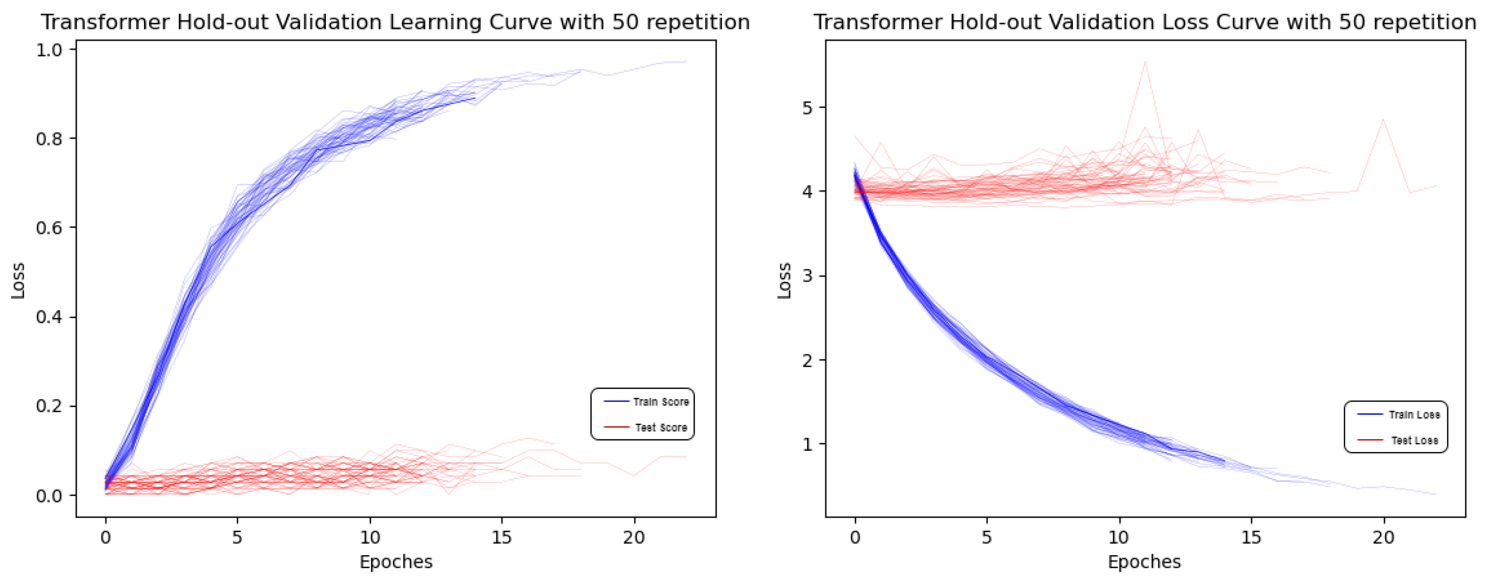
4.2. Transformer Result

The transformer is mainly used for language translation [58] and time sequence forecasting [59], which means it can be used as the baseline model for comparison. While there is a significant amount of research related to time series forecasting, there is a limited amount of research on time series classification, particularly for multi-class classification tasks such as in-air signature recognition. Nevertheless, Ford Car company released a motor noise classification dataset, which is a binary time sequence classification task [60]. A transformer can be used to classify whether the given motor sound signal contains the damaged part, and the whole labeling set is marked as “damaged” or “undamaged”. The dataset (proposed in 2018) includes 3601 training samples and 1320 testing samples with only 2 classes. There would be 1800 training samples for each class and 660 testing samples for each class if the classes are balanced. This transformer model can be further developed into a multi-classification time sequence model for smartwatch in-air signature recognition. As shown in Figure 15, the original length of 440 concatenated in-air signature signals is recorded.

To best exploit the performance of the transformer, the nine-dimensional smartwatch in-air signature data were downsampled with the corresponding frequency for each dimension to fit the shortest signal length and concatenated together for each time stamp, which was of the length 1400. Then each time stamp in-air signature signals were normalized with respect to the summation of the current time stamp. As shown in Table 4 and Table 5, the transformer works as the baseline model for comparison. The dropout is set to 0.25, and layer-normalization is specified as $1e^{-6}$ for the model to reduce the effect of over-fitting, but the over-fitting problem exists to a different degree among 50 repetitions, as shown in Figure 16.

The learning curve of the training set shows high accuracy and reaches over 90% for some optimizers, indicating the model is, in fact, learning pattern knowledge during the epochs. However, the testing accuracy stays low, which means that this knowledge is difficult to generalize over new samples. The main reason for this is that the transformer works on very large amounts of data [59,61,62], and its performance is dependent on pre-training. For example, BERT uses Wikipedia for the pre-training and it performs well for the downstream language processing tasks [58]. The transformer is a-complicated structure with too many parameters involved [63] and over-fitting is expected, given a small- or medium-sized dataset. For the time sequence recognition model, a simpler model with lower complexity, such as DTW [14] and LSTM [22], would be more desirable. In Li’s research, LSTM and RNN show effective performances with 0.83% and 0.97% EER, respectively [4]. In our research, convolutional neural networks can be much easier to generalize on small- or medium-sized in-air signature datasets without pre-training. Additionally, using CNN for in-air signature recognition is popular for a moderately sized dataset [5,64,65]. In Behera’s research [8], the experiment uses self-designed CNN for in-air signature recognition; a moderately sized dataset (50 participants) was used for the experiment. The results showed 4% improvement compared with the time sequence model, such as the LSTM model.

5. Discussion

The experiment shows that the optimizer has a significant influence on loss and accuracy in median-sized in-air signature classification tasks. After fine-tuning the learning rate and optimizer, we can obtain the best testing performance score.

Table 6. The table shows the best performance configuration that was tested in this experiment for each model and the corresponding testing score in percentage. Please note that the experiment does not enumerate every combination of parameters exhaustively. In theory, there is still a possible combination that gives a better performance for each model.

Final Configuration for Each Model
	LeNet	AlexNet	VGG	ResNet	Transformer (Baseline)
Learning Rate	$1\times {10}^{-1}$	$1\times {10}^{-4}$	$1\times {10}^{-4}$	$1\times {10}^{-4}$	$1\times {10}^{-4}$
Optimizer	SGD	Adamax	Adamax	Adagrad	Adamax
Test Score (%)	99.4086	99.4232	99.5205	99.8514	0.1268

shows the best configuration for each of the models when applied to the smartwatch in-air signature dataset. The ResNet model with a learning rate of $1\times {10}^{-4}$ and Adagrad as the optimizer gives the best performance of 99.8514% for the smartwatch in-air signature testing dataset.

Figure 17 and Figure 18 show the learning and loss curves for four models in 1000 Epochs. The ResNet is the gray colored line, from which we could observe that ResNet shows a much better tendency compared with the rest of the models.

6. Future Research

In-air signature recognition using the in-air signatures of only 22 participants is a relatively small dataset; this should be expanded in the near future and a comparison among the real handwritten signature will be conducted. The statistical ablation study would be very helpful in investigating further. We could statistically observe which part of the CNN provides better performance for the in-air signature dataset by removing certain blocks within the CNN. Analyzing statistically or mathematically the relatively high-performance CNN originating from the layer or sub-structure would be a great direction for future research. More time sequence models and convolution neural networks should be tested. Moreover, wearable intelligent gloves can be used to detect the in-air signature signals as well, and Raspberry Pi [66] can be used to build this device from scratch; we could have the flexibility and freedom of choosing the more reliable sensors, and the applications can also be expanded to sign language recognition and virtual reality (VR) [67].

7. Conclusions

In this research, we used the smartwatch in-air signature dataset consisting of 22 participants with 10 genuine signatures and 10 fake signatures, which were composed of 440 in-air signatures and 44 classifications. We performed the dynamic time warping algorithm (DTW) to verify the usability of the dataset. The nine-dimensional raw data went through normalization, concatenation, and downsampling as the data pre-processing for transformers, but it showed different degrees of overfitting for various combinations of optimizers and learning rates. We performed three-dimensional static restoration of the in-air signature data from the smartwatch to fit convolutional neural network models. Four convolutional models, including the LeNet, AlexNet, VGG, and ResNet, were tested with respect to 10 optimizers, including Adadelta, Adagrad, Adam, AdamW, Adamax, ASGD, NAdam, RAdam, RMSprop, and SGD. In our experiment, the best testing performance achieved a successful prediction rate of 99.8514% for the identity category of the in-air signature signer using ResNet with the Adagrad optimizer and a learning rate of $1\times {10}^{-4}$.

References

1. Oğuz, A.; Ertuğrul, Ö.F. Human identification based on accelerometer sensors obtained by mobile phone data. Biomed. Signal Process. Control 2022, 77, 103847. [Google Scholar] [CrossRef]
2. Ketabdar, H.; Moghadam, P.; Naderi, B.; Roshandel, M. Magnetic signatures in air for mobile devices. In Proceedings of the 14th International Conference on Human-Computer Interaction with Mobile Devices and Services Companion, San Francisco, CA, USA, 21–24 September 2012; pp. 185–188. [Google Scholar]
3. Rehman, W.U.; Laghari, A.; Memon, Z.U. Exploiting smart phone accelerometer as a personal identification mechanism. Mehran Univ. Res. J. Eng. Technol. 2015, 34, 21–26. [Google Scholar]
4. Li, G.; Sato, H. Sensing in-air signature motions using smartwatch: A high-precision approach of behavioral authentication. IEEE Access 2022, 10, 57865–57879. [Google Scholar] [CrossRef]
5. Malik, J.; Elhayek, A.; Ahmed, S.; Shafait, F.; Malik, M.I.; Stricker, D. 3dairsig: A framework for enabling in-air signatures using a multi-modal depth sensor. Sensors 2018, 18, 3872. [Google Scholar] [CrossRef] [Green Version]
6. Fang, Y.; Kang, W.; Wu, Q.; Tang, L. A novel video-based system for in-air signature verification. Comput. Electr. Eng. 2017, 57, 1–14. [Google Scholar] [CrossRef]
7. Guerra-Segura, E.; Ortega-Pérez, A.; Travieso, C.M. In-air signature verification system using leap motion. Expert Syst. Appl. 2021, 165, 113797. [Google Scholar] [CrossRef]
8. Behera, S.K.; Dash, A.K.; Dogra, D.P.; Roy, P.P. Air signature recognition using deep convolutional neural network-based sequential model. In Proceedings of the 2018 24th International Conference on Pattern Recognition (ICPR), Beijing, China, 20–24 August 2018; pp. 3525–3530. [Google Scholar]
9. Wang, H.; Lymberopoulos, D.; Liu, J. Sensor-based user authentication. In Wireless Sensor Networks; Abdelzaher, T., Pereira, N., Tovar, E., Eds.; Springer International Publishing: Cham, Switzerland, 2015; pp. 168–185. [Google Scholar]
10. Laghari, A.; Waheed-ur-Rehman; Memon, Z.A. Biometric authentication technique using smartphone sensor. In Proceedings of the 2016 13th International Bhurban Conference on Applied Sciences and Technology (IBCAST), Islamabad, Pakistan, 12–16 January 2016; pp. 381–384. [Google Scholar]
11. Vaswani, A.; Shazeer, N.; Parmar, N.; Uszkoreit, J.; Jones, L.; Gomez, A.N.; Kaiser, L.; Polosukhin, I. Attention is all you need. arXiv 2017, arXiv:1706.03762. [Google Scholar]
12. Rumelhart, D.E.; Hinton, G.E.; Williams, R.J. Learning internal representations by error propagation. Parallel Distrib. Process. 1986, 1, 318–363. [Google Scholar]
13. Li, Z.; Liu, F.; Yang, W.; Peng, S.; Zhou, J. A survey of convolutional neural networks: Analysis, applications, and prospects. IEEE Trans. Neural Netw. Learn. Syst. 2022, 33, 6999–7019. [Google Scholar] [CrossRef]
14. Sakoe, H.; Chiba, S. Dynamic programming algorithm optimization for spoken word recognition. IEEE Trans. Acoust. Speech Signal Process. 1978, 26, 43–49. [Google Scholar] [CrossRef] [Green Version]
15. Lecun, Y.; Bottou, L.; Bengio, Y.; Haffner, P. Gradient-based learning applied to document recognition. Proc. IEEE 1998, 86, 2278–2324. [Google Scholar] [CrossRef] [Green Version]
16. Krizhevsky, A.; Sutskever, I.; Hinton, G.E. Imagenet classification with deep convolutional neural networks. Commun. ACM 2017, 60, 84–90. [Google Scholar] [CrossRef] [Green Version]
17. Simonyan, K.; Zisserman, A. Very deep convolutional networks for large-scale image recognition. arXiv 2014, arXiv:1409.1556. [Google Scholar]
18. He, K.; Zhang, X.; Ren, S.; Sun, J. Deep residual learning for image recognition. arXiv 2015, arXiv:1512.03385. [Google Scholar]
19. Kiernan, M.C.; Vucic, S.; Cheah, B.C.; Turner, M.R.; Eisen, A.; Hardiman, O.; Burrell, J.R.; Zoing, M.C. Amyotrophic lateral sclerosis. Lancet 2011, 377, 942–955. [Google Scholar] [CrossRef] [Green Version]
20. Xie, Z.; Schwartz, O.; Prasad, A. Decoding of finger trajectory from ecog using deep learning. J. Neural Eng. 2017, 15, 11. [Google Scholar] [CrossRef]
21. Fukushima, K. Neocognitron: A self-organizing neural network model for a mechanism of pattern recognition unaffected by shift in position. Biol. Cybern. 1980, 36, 193–202. [Google Scholar] [CrossRef]
22. Hochreiter, S.; Schmidhuber, J. Long short-term memory. Neural Comput. 1997, 9, 1735–1780. [Google Scholar] [CrossRef]
23. Pfurtscheller, G.; Müller, G.R.; Pfurtscheller, J.; Gerner, H.J.; Rupp, R. ‘Thought’—Control of functional electrical stimulation to restore hand grasp in a patient with tetraplegia. Neurosci. Lett. 2003, 351, 33–36. [Google Scholar] [CrossRef]
24. Guerra-Casanova, J.; Sánchez-Ávila, C.; de Santos-Sierra, A.; Bailador, G. A robustness verification system for mobile phone authentication based on gestures using linear discriminant analysis. In Proceedings of the 2011 Third World Congress on Nature and Biologically Inspired Computing, Salamanca, Spain, 19–21 October 2011; pp. 157–162. [Google Scholar]
25. Guerra-Casanova, J.; Ávila, C.S.; Bailador, G.; de-Santos-Sierra, A. Time series distances measures to analyze in-air signatures to authenticate users on mobile phones. In Proceedings of the 2011 Carnahan Conference on Security Technology, Barcelona, Spain, 18–21 October 2011; pp. 1–7. [Google Scholar]
26. Khoh, W.H.; Pang, Y.H.; Teoh, A.B. In-air hand gesture signature recognition system based on 3-dimensional imagery. Multimed. Tools Appl. 2019, 78, 6913–6937. [Google Scholar] [CrossRef]
27. Wang, S.; Yuan, J.; Wen, J. Adaptive phone orientation method for continuous authentication based on mobile motion sensors. In Proceedings of the 2019 IEEE 31st International Conference on Tools with Artificial Intelligence (ICTAI), Portland, OR, USA, 4–6 November 2019; pp. 1623–1627. [Google Scholar]
28. Buriro, A.; Crispo, B.; Delfrari, F.; Wrona, K. Hold and sign: A novel behavioral biometrics for smartphone user authentication. In Proceedings of the 2016 IEEE Security and Privacy Workshops (SPW), San Jose, CA, USA, 22–26 May 2016; pp. 276–285. [Google Scholar]
29. Primo, A.; Phoha, V.V.; Kumar, R.; Serwadda, A. Context-aware active authentication using smartphone accelerometer measurements. In Proceedings of the 2014 IEEE Conference on Computer Vision and Pattern Recognition Workshops, Columbus, OH, USA, 23–28 June 2014; pp. 98–105. [Google Scholar]
30. Saleem, M.; Kovari, B. Survey of signature verification databases. In Proceedings of the MultiScience—XXXIII microCAD International Multidisciplinary Scientific Conference, Miskolc, Hungary, 23–24 May 2019. [Google Scholar]
31. Bailador, G.; Sanchez-Avila, C.; Guerra-Casanova, J.; de Santos Sierra, A. Analysis of pattern recognition techniques for in-air signature biometrics. Pattern Recognit. 2011, 44, 2468–2478. [Google Scholar] [CrossRef] [Green Version]
32. Yeo, K.; Yin, O.S.; Han, P.Y.; Kwee, W.K. Real time mobile application of in-air signature with fast dynamic time warping (fastdtw). In Proceedings of the 2015 IEEE International Conference on Signal and Image Processing Applications (ICSIPA), Kuala Lumpur, Malaysia, 19–21 October 2015; pp. 315–320. [Google Scholar]
33. Muscillo, R.; Conforto, S.; Schmid, M.; Caselli, P.; D’Alessio, T. Classification of motor activities through derivative dynamic time warping applied on accelerometer data. In Proceedings of the Conference proceedings: Annual International Conference of the IEEE Engineering in Medicine and Biology Society, Lyon, France, 22–26 August 2007; Volume 2007, pp. 4930–4933. [Google Scholar]
34. Mantena, G.; Achanta, S.; Prahallad, K. Query-by-example spoken term detection using frequency domain linear prediction and nonsegmental dynamic time warping. IEEE/ACM Trans. Audio Speech Lang. Process. 2014, 22, 946–955. [Google Scholar] [CrossRef]
35. Furlanello, C.; Merler, S.; Jurman, G. Combining feature selection and dtw for time-varying functional genomics. IEEE Trans. Signal Process. 2006, 54, 2436–2443. [Google Scholar] [CrossRef]
36. Müller, M. Information Retrieval for Music and Motion; Springer: Berlin/Heidelberg, Germany, 2007. [Google Scholar]
37. Schaller, M.; Gonnet, P.; Draper, P.W.; Chalk, A.B.; Bower, R.G.; Willis, J.; Hausammann, L. SWIFT: SPH with Inter-Dependent Fine-Grained Tasking; Astrophysics Source Code Library: Online, 2018; ascl:1805.020. [Google Scholar]
38. Zeiler, M.D. Adadelta: An adaptive learning rate method. arXiv 2012, arXiv:1212.5701. [Google Scholar]
39. Duchi, J.; Hazan, E.; Singer, Y. Adaptive subgradient methods for online learning and stochastic optimization. J. Mach. Learn. Res. 2011, 12, 2121–2159. [Google Scholar]
40. Diederik, K.; Jimmy, B. Adam: A method for stochastic optimization. arXiv 2014, arXiv:1412.6980. [Google Scholar]
41. Loshchilov, I.; Hutter, F. Decoupled weight decay regularization. arXiv 2017, arXiv:1711.05101. [Google Scholar]
42. Polyak, B.T.; Juditsky, A.B. Acceleration of stochastic approximation by averaging. SIAM J. Control Optim. 1992, 30, 838–855. [Google Scholar] [CrossRef] [Green Version]
43. McMahan, B. Follow-the-regularized-leader and mirror descent: Equivalence theorems and l1 regularization. In Proceedings of the Fourteenth International Conference on Artificial Intelligence and Statistics, Fort Lauderdale, FL, USA, 11–13 April 2011; Volume 15, pp. 525–533. [Google Scholar]
44. Dozat, T. Incorporating Nesterov Momentum into Adam. In Proceedings of the 4th International Conference on Learning Representations, San Juan, Puerto Rico, 2–4 May 2016; pp. 1–4. [Google Scholar]
45. Liu, L.; Jiang, H.; He, P.; Chen, W.; Liu, X.; Gao, J.; Han, J. On the variance of the adaptive learning rate and beyond. arXiv 2019, arXiv:1908.03265. [Google Scholar]
46. Graves, A. Generating sequences with recurrent neural networks. arXiv 2013, arXiv:1308.0850. [Google Scholar]
47. Sutskever, I.; Martens, J.; Dahl, G.; Hinton, G. On the importance of initialization and momentum in deep learning. In Proceedings of the 30th International Conference on Machine Learning, ser. Proceedings of Machine Learning Research, Atlanta, GA, USA, 17–19 June 2013; Dasgupta, S., McAllester, D., Eds.; PMLR: Cambridge, MA, USA, 2013; Volume 28, pp. 1139–1147. [Google Scholar]
48. Fukushima, K. Cognitron: A self-organizing multilayered neural network. Biol. Cybern. 1975, 20, 121–136. [Google Scholar] [CrossRef]
49. Deng, J.; Dong, W.; Socher, R.; Li, L.-J.; Li, K.; Fei-Fei, L. Imagenet: A large-scale hierarchical image database. In Proceedings of the 2009 IEEE Conference on Computer Vision and Pattern Recognition, Miami, FL, USA, 20–25 June 2009; pp. 248–255. [Google Scholar]
50. Smith, L.N. Cyclical Learning Rates for Training Neural Networks. 2015. Available online: https://arxiv.org/abs/1506.01186 (accessed on 10 February 2023).
51. Kaur, H.; Pannu, H.S.; Malhi, A.K. A systematic review on imbalanced data challenges in machine learning: Applications and solutions. ACM Comput. Surv. (CSUR) 2019, 52, 79. [Google Scholar] [CrossRef] [Green Version]
52. Chollet, François and others; Keras. 2015. Available online: https://github.com/fchollet/keras (accessed on 10 February 2023).
53. Paszke, A.; Gross, S.; Massa, F.; Lerer, A.; Bradbury, J.; Chanan, G.; Killeen, T.; Lin, Z.; Gimelshein, N.; Antiga, L.; et al. Pytorch: An imperative style, high-performance deep learning library. In Advances in Neural Information Processing Systems 32; Curran Associates, Inc.: Cambridge, MA, USA, 2019; pp. 8024–8035. Available online: http://papers.neurips.cc/paper/9015-pytorch-an-imperative-style-high-performance-deep-learning-library.pdf (accessed on 10 February 2023).
54. Cui, K.; Zhan, Z.; Pan, C. Applying radam method to improve treatment of convolutional neural network on banknote identification. In Proceedings of the 2020 International Conference on Computer Engineering and Application (ICCEA), Guangzhou, China, 18–20 March 2020; pp. 468–476. [Google Scholar]
55. Ariff, N.A.M.; Ismail, A.R. Study of adam and adamax optimizers on alexnet architecture for voice biometric authentication system. In Proceedings of the 2023 17th International Conference on Ubiquitous Information Management and Communication (IMCOM), Seoul, Republic of Korea, 3–5 January 2023; pp. 1–4. [Google Scholar]
56. Lorencin, I. Urinary bladder cancer diagnosis using customized vgg-16 architectures. Sarcoma 2022, 10, 11. [Google Scholar]
57. Yang, J.; Bagavathiannan, M.; Wang, Y.; Chen, Y.; Yu, J. A comparative evaluation of convolutional neural networks, training image sizes, and deep learning optimizers for weed detection in alfalfa. Weed Technol. 2022, 36, 512–522. [Google Scholar] [CrossRef]
58. Devlin, J.; Chang, M.-W.; Lee, K.; Toutanova, K. Bert: Pre-training of deep bidirectional transformers for language understanding. arXiv 2018, arXiv:1810.04805. [Google Scholar]
59. Wu, N.; Green, B.; Ben, X.; O’Banion, S. Deep transformer models for time series forecasting: The influenza prevalence case. arXiv 2020, arXiv:2001.08317. [Google Scholar]
60. Wichard, J.D. Classification of Ford Motor Data. Computer Science. 2008. Available online: https://www.semanticscholar.org/paper/Classification-of-Ford-Motor-Data-Wichard/7a7b1674a126db6836337cf9164c0522465f76fc#related-papers (accessed on 10 February 2023).
61. Wu, S.; Xiao, X.; Ding, Q.; Zhao, P.; Wei, Y.; Huang, J. Adversarial sparse transformer for time series forecasting. In Advances in Neural Information Processing Systems; Larochelle, H., Ranzato, M., Hadsell, R., Balcan, M., Lin, H., Eds.; Curran Associates, Inc.: Cambridge, MA, USA, 2020; Volume 33, pp. 17105–17115. [Google Scholar]
62. Cai, L.; Janowicz, K.; Mai, G.; Yan, B.; Zhu, R. Traffic transformer: Capturing the continuity and periodicity of time series for traffic forecasting. Trans. GIS 2020, 24, 736–755. [Google Scholar] [CrossRef]
63. Zhai, X.; Kolesnikov, A.; Houlsby, N.; Beyer, L. Scaling vision transformers. In Proceedings of the IEEE/CVF Conference on Computer Vision and Pattern Recognition (CVPR), New Orleans, LA, USA, 18–24 June 2022; pp. 12104–12113. [Google Scholar]
64. Sasipriyaa, N.; Natesan, P.; Mohana, R.; Gothai, E.; Venu, K.; Mohanapriya, S. Design and simulation of handwritten detection via generative adversarial networks and convolutional neural network. Mater. Today Proc. 2021, 47, 6097–6100. Available online: https://www.sciencedirect.com/science/article/pii/S2214785321036002 (accessed on 10 February 2023). [CrossRef]
65. Ghosh, S.; Ghosh, S.; Kumar, P.; Scheme, E.; Roy, P.P. A novel spatio-temporal siamese network for 3d signature recognition. Pattern Recognit. Lett. 2021, 144, 13–20. [Google Scholar] [CrossRef]
66. Upton, E.; Halfacree, G. Raspberry Pi User Guide; John Wiley & Sons: Hoboken, NJ, USA, 2014. [Google Scholar]
67. Schuemie, M.J.; Straaten, P.V.D.; Krijn, M.; Van Der Mast, C.A. Research on presence in virtual reality: A survey. Cyberpsychol. Behav. 2001, 4, 183–201. [Google Scholar] [CrossRef]
Figure 1. Experiment System architecture for a smartwatch’s in-air recognition. Please note the data collection phase using swift was conducted by Li [4] in his previous research. The convolutional layer experiment section is based on AlexNet [16], LeNet [15], VGG [17], and ResNet [18]. The transformer experiment section is based on the original transformer paper [11].
Applsci 13 03958 g001
Figure 2. Smartwatch accelerometer data of 10 genuine signature signals from the same participant.
Applsci 13 03958 g002
Figure 3. Dynamic Time Warping Alignment of two signature signals. The blue line and the orange line represent two signatures respectively while the yellow line shows alignment.
Applsci 13 03958 g003
Figure 4. Dynamic time warping cost matrix of two signature signals.
Applsci 13 03958 g004
Figure 5. The genuine and forged in-air signature DTW distance comparisons of the smartwatch. PXR represents the DTW distance of the genuine signatures of participant X, and PXF represents the DTW distance of the forgery signatures of participant X. The yellow dots demonstrates the specific DTW alignment costs among the two signatures.
Applsci 13 03958 g005
Figure 6. Gray-scale in-air signature of a 32 by 32 transformation and the three-channel RGB in-air signature of a 224 by 224 transformation.
Applsci 13 03958 g006
Figure 7. LeNet-5 structure.
Applsci 13 03958 g007
Figure 8. AlexNet structure.
Applsci 13 03958 g008
Figure 9. VGG-16 structure (D configuration).
Applsci 13 03958 g009
Figure 10. The in-air signature three-dimensional static restoration of a smartwatch.
Applsci 13 03958 g010
Figure 11. The loss curve of LeNet with respect to 10 different optimizers. Both the learning loss and testing loss for each optimizer are covered in the graph. The two zoom-in areas are ( x 1 , x 2 ) = (0, 1000), ( y 1 , y 2 ) = (3, 4); ( x 1 , x 2 ) = (0, 300), ( y 1 , y 2 ) = (0, 2).
Applsci 13 03958 g011
Figure 12. The loss curve of AlexNet with respect to 10 different optimizers. Both the learning loss and testing loss for each optimizer are covered in the graph. The zoom-in area is ( x 1 , x 2 ) = (0, 100), ( y 1 , y 2 ) = (0, 4).
Applsci 13 03958 g012
Figure 13. The loss curve of VGG with respect to 10 different optimizers. Both the learning loss and testing loss for each optimizer are covered in the graph. The zoom-in area is ( x 1 , x 2 ) = (0, 100), ( y 1 , y 2 ) = (0, 4).
Applsci 13 03958 g013
Figure 14. The loss curve of ResNet with respect to 10 different optimizers. Both the learning loss and testing loss for each optimizer are covered in the graph. The zoom-in area is ( x 1 , x 2 ) = (0, 100), ( y 1 , y 2 ) = (0, 4).
Applsci 13 03958 g014
Figure 15. The in-air signature nine-dimensional concatenated length of a smartwatch.
Applsci 13 03958 g015
Figure 16. Transformer over-fitting phenomena on smartwatch dataset in 50 repetitions.
Applsci 13 03958 g016
Figure 17. Learning curve comparisons for the LeNet training process, LeNet testing process, AlexNet training process, AlexNet testing process, VGG training process, VGG testing process, ResNet training process, and ResNet testing process.
Applsci 13 03958 g017
Figure 18. Loss curve comparisons for the LeNet training process, LeNet testing process, AlexNet training process, AlexNet testing process, VGG training process, VGG testing process, ResNet training process, and ResNet testing process.
Applsci 13 03958 g018