Efficient Computer-Based Method for Adjusting the Stiffness of Subject-Specific 3D-Printed Insoles during Walking

Featured Application

Quasi-static finite element model to adjust the stiffness of 3D-printed insoles during walking for patients with diabetic foot by using ankle moments and joint reaction forces as efficient boundary conditions.

Abstract

Diabetes-adapted insoles are essential in prevention and rehabilitation of foot ulcers in diabetic foot syndrome. However, their manufacture is labour-intensive and costly. Therefore, the study aims to present an alternative method that allows the individual adjustment of the stiffness of the insoles using the finite element (FE) method and subsequent 3D printing. In the study, 3D gait analysis followed by musculoskeletal modelling was used to determine the boundary conditions of a healthy subject for the FE model. While muscle forces are elaborately implemented in most studies, this FE model presented a more efficient way by using ankle moments and joint reaction forces. The deviation between the simulated plantar peak pressure and the experimentally determined using the Pedar system amounted to 234 kPa in the heel area and 30 kPa in the toe area. The stiffness of the individual insole was adjusted by applying soft insole plugs in areas where high plantar pressures occurred during walking. Three different Young’s moduli were analysed in these areas (0.5 MPa, 1.0 MPa, 1.5 MPa). The computer-based approach to adjust the stiffness of an individual insole revealed a plantar peak pressure reduction by 37% in the heel area and by 119% in the toe area with a Young’s modulus of 0.5 MPa. The presented method could be a valuable tool in the cost-efficient development and engineering of subject-specific 3D-printed insoles for patients with diabetic foot syndrome.

1. Introduction

The current global number of people with diabetes mellitus is approximately 536 million and is estimated to increase to 700 million by 2045 [1]. This will also increase the incidence of diabetic foot syndrome [2]. Here, foot ulceration is the most common complication [3]. The main risk factor for the development of foot ulceration is diabetic polyneuropathy. The associated altered plantar pressure decreases pain sensation and altered skin function in combination with abnormal repetitive pressure overload and causes foot ulcers. An additional major problem of diabetic foot syndrome is the high ulcer recurrence rate. Here, a history of foot ulceration is among the greatest risk factors [4]. The probability of recurrence after an healed ulcer within one year is 40%, but it is 65% after three years [3]. As foot ulcers recur, the likelihood of minor and major amputation also increases [5,6,7]. Therefore, diabetic foot ulceration is associated with a high rate of lower extremity amputation and is among the major causes of mobility impairment worldwide [2,8,9,10]. Prevention and remission measures are becoming increasingly important to reduce the first occurrence of an ulcer and the recurrence rate [11,12].

A major aim is to reduce the increased plantar pressure associated with diabetic foot syndrome using specific shoe and insole care [11,12,13,14,15,16,17,18]. In this context, customized insoles, so-called diabetes-adapted insoles, play an important role [13,17]. However, the conventional production of these diabetes-adapted insoles is time-consuming [19]. The insoles are adjusted for shape and stiffness over multiple patient trials by removing and filling material until the desired reduction in peak plantar pressure is achieved. The increased effort is ultimately accompanied by increased costs as well [20,21]. Additionally, the available materials are limited in terms of their mechanical properties [19]. The finite element (FE) method, combined with additive manufacturing processes, represents a promising alternative, as the method enables insole customization via parametric analysis. Additive manufacturing processes can directly produce the insoles that have been adapted in shape and stiffness. Moreover, they offer a more comprehensive range of physical material properties by changing the internal structure and filling degree of the 3D-printed material [19].

Currently, various FE models exist that simulate the plantar pressure distribution between the foot and the insole in order to investigate the influence of different sole designs and modifications, or to adjust the sole stiffness. These models greatly differ in their complexity. From a clinical application, the FE model should be as simple as possible, but as complex as necessary [22,23]. Both 2D and 3D models have been described [24,25,26,27,28,29,30,31,32,33,34,35]; the former has a lower computational time to advantage, so dynamic analyses are mostly used [24,25]. However, a disadvantage of 2D models is the limited analysis area. Therefore, recent studies have used static or quasi-static 3D simulations [27,28,29,30,31,32,33,34,35]. Although the International Working Group of Diabetic Foot recommends adjusting the stiffness of diabetes-adapted insoles based on the plantar pressure distribution during gait [13,17], most studies analysed plantar pressure during a balanced stance, and only some studies have simulated a gait cycle [27,32,35]. FE models that analyse gait or time points of gait are usually very complex due to the detailed geometries (joints, cartilages, ligaments, etc.) and the integration of muscle forces [27,29,30,32,35,36,37]. Furthermore, the implementation of muscle forces proves to be challenging and unsuitable for daily clinical practice [22,38].

In this context, Peng et al. [32] investigated the plantar pressure distribution between the insole and the foot by simulating three different time points of the gait. Subject-specific boundary conditions, i.e., muscle forces and ground reaction force, determined by gait analysis and a subsequent musculoskeletal multibody simulation, were applied to the FE model. The individual bones were reconstructed from magnetic resonance imaging (MRI) data and ligaments, plantar fascia and muscle connectors were considered. For clinical practice, this would be too labour-intensive and time-consuming, and would not represent a reduction in workload. On the other hand, Su et al. [33] used simplified boundary conditions, but only analysed the plantar pressure distribution during the stance phase. In line with Peng et al. [32], a very detailed foot model, i.e., individual bones, cartilage, ligaments, skin, and soft tissues, reconstructed from CT data, were considered. Contrarily, Tang et al. [34] used a simplified foot model, i.e., bones of the foot, reconstructed from CT data, which were merged as one geometry. However, they also used simplified boundary conditions for stance and not for gait. These examples show the need for a simplified model with simplified structures and subject-specific boundary conditions of walking, which can be used for additive manufacturing in this field to reduce the amount of work and time required. Reviews have also highlighted the need for an established method for clinical application [22,23]. In addition, there have been few studies that adjusted the stiffness of 3D-printed insoles using the FE method [32,34].

Therefore, our present study aimed to develop an efficient FE model of the foot that enables the stiffness adjustment of an individual insole and its subsequent additive manufacturing. The stiffness adjustment should be based on the plantar pressure distribution during normal walking. For this purpose, ankle joint reaction forces and moments from a subject were integrated into the FE model based on a 3D gait analysis with subsequent musculoskeletal multibody modelling.

2. Materials and Methods

2.1. Participant Information and Construction of the Insole

The fitting of an individual left insole was performed for a test person of 27 years old (body weight: 72.5 kg; height: 1.76 m), who did not suffer from diabetic foot syndrome or foot deformity. Ethical approval was granted by the Ethics Committee of the Rostock University Medical Center, Germany (A 2023-0021).

To digitally fit the shape of the insole to the subject’s foot, the foot surface was scanned using the UPOD-S 3D laser scanner (Scan-Pod3D, Wuhan, China). Here, the foot surface was recorded in a seated position with the knee and foot at a 90-degree angle. This only partially loaded position of the foot allows the natural shape of the foot to be recorded [39]. Based on these digital foot surfaces, the insoles were designed using the CAD programme FootMILL-CAD (Systemic & FootMILL-CAD, Flensburg, Germany). The shape of the insole was based on the external shape of the foot. A thickness of 8 mm was chosen for the thinnest part of the diabetes-adapted insole. The insole was fitted to a special shoe model for people with diabetes called EVA (model No.: 251004, LucRo by Schein, Remscheid, Germany).

The digitally designed insoles were simultaneously used to manufacture the 3D-printed insoles from a thermoplastic copolyester with the IPT-Printer (Raise 3D PRO2, Raise 3D Technologies, Inc., Irvine, CA, USA). The filament thickness was 2.85 mm. Printing was performed at a temperature of 225 °C. The printing speed was 40 mm/s for the filling structure and 20 mm/s for the outer wall. The additively manufactured insoles had a gyroid filling structure with a filling of 20%. The top and bottom thicknesses were 1.1 mm, and the wall layer was 1.6 mm thick.

2.2. Gait Measurements

The 3D gait analysis (Figure 1) was performed using the Gait Realtime Analysis Interactive Lab (GRAIL) (Motek Medical B.V., Houten, The Netherlands), a fully integrated treadmill with motion analysis systems. It was equipped with ten Vicon cameras (Vicon, Oxford Metrics Ltd., Oxford, England) and two AMTI force plates (OR6, AMTI, Watertown, MA, USA) so that marker trajectories and ground reaction forces could be recorded [40,41]. Following the modified human body model for clinical lower extremity gait analysis from Motek (Motek Medical B.V., Houten, The Netherlands) [42], reflectable infrared markers were attached to the bony landmarks of the subject. Plantar pressure data were simultaneously collected during the 3D gait analysis using Pedar pressure measurement insoles (Pedar-x system, Novel GmbH, Munich, Germany), enabling subsequent validation of the FE model by comparing [31]. For this purpose, the pressure measurement insoles were inserted into the shoes together with the additively manufactured insoles. Data were recorded at normal gait speed, as it has been recommended to fit diabetes-adapted insoles based on plantar pressure distributions during this movement [13,17]. The identified comfort speed was 1.29 m/s. The subject had sufficient time to familiarize with the experimental environment and achieve a natural gait, followed by a one-minute recorded trial. The sampling frequency of the motion capture system and ground reaction forces was 100 Hz and 1000 Hz, respectively. The pressure measurement insoles recorded the plantar pressures at the maximum possible frequency of 100 Hz. The gait data were used for a subsequent musculoskeletal multibody simulation of the lower extremity.

2.3. Musculoskeletal Multibody Model

The obtained ground reaction forces and marker trajectories of the 3D gait analysis were imported into a musculoskeletal multibody model to determine the boundary conditions, i.e., joint forces and moments, for the FE model. The AnyBody software package (version 6.0.5, AnyBody Technology, Aalborg, Denmark) with the MoCap Lower Extremity Model included in the AnyBody Managed Model Repository, version 2.3.4, was used to create the subject-specific musculoskeletal multibody model [43,44]. In this model, the ankle joint has two lines of freedom: eversion/inversion and flexion/extension. Experimental data were filtered using a 7.0 Hz second-order Butterworth low-pass filter. Parameter optimization was used to fit the generic model to the anthropometric data of the subject. An inverse kinematics analysis was performed to calculate the joint angles of the lower extremity. These joint angles and the ground reaction forces were used as input for an inverse dynamics analysis to determine the joint moments and joint reaction forces [45]. The inverse dynamics were performed without including the muscle forces, since no acting muscle forces were simulated in the FE model [46,47] (Figure 2).

Further processing of the data calculated in the musculoskeletal multibody simulation was performed in Matlab R2019b (The MathWorks Inc., Natick, MA, USA). All forces and moments were transformed in the local calcaneus coordinate system according to Wu et al. [48], which is defined by anatomical landmarks. It is attached to the foot segment so that its orientation does not change during the mid-stance phase. Mean values were taken from 15 recorded steps where the foot was entirely within the force plates. In the FE analysis, the time points of the early and late mid-stance phases were used. These time points allow the insoles to be adjusted in areas where plantar pressure peaks occur in both the forefoot and rearfoot without considerably changing foot position. The early and late mid-stance phases roughly correspond to the first high and low points of the vertical ground reaction force, respectively.

2.4. Finite Element Modelling

2.4.1. Geometries

MRI (Skyra Fit, Siemens, Erlangen, Germany) data with a voxel size of 1.5 mm were used as the basis for the 3D reconstruction of the subject foot and skeleton geometry. The foot was positioned perpendicular at a 90-degree angle to the thigh against a plate during the MRI. Segmentation of the geometries was performed using Amira software (version 5.4.1, Zuse Institute Berlin, Berlin, Germany; Thermo Fisher Scientific, Waltham, MA, USA). To simplify the FE model, the relative motions of the individual bones to each other were neglected. For this purpose, the joints were merged so that the skeleton finally consisted of a single geometry. In order to ensure an exact alignment of the foot skeleton within the foot surface, the outer foot surface was also segmented from the MRI images. Further processing and creation of a solid model were performed in Geomagic Studio 2013 (3D Systems, Rock Hill, SC, USA) according to an established workflow [49]. The foot geometry was trimmed parallel to the body transverse plane so that the talus was exposed when the foot and skeletal geometry were merged. This allows the force to be applied to the talus bone in the FE model.

All geometries and the calcaneus coordinate system were imported into Abaqus (version 6.14, Dassault Systèmes Simulia Corp., Providence, RI, USA). In addition, another geometry, the shoe sole with a thickness of 20 mm (approximately the height of the sole of the diabetic shoe model), was constructed. The foot skeleton and foot surface were merged and the insole was tied to the shoe sole (Figure 3).

2.4.2. Material Properties

Experimental compression tests were carried out to determine the elastic modulus of the additively manufactured insole. The force-displacement curves of three cylindrical specimens (height 8 mm, diameter 60 mm) were measured using the ZwickRoell testing machine (ZwickRoell AG, Ulm, Germany) and its testing software, testXpert 2 (ZwickRoell AG, Ulm, Germany). The compression test was based on the compression test standard ASTM D 3574-17 [50], with a compression speed of 1 mm/min; the trial ended at 25% of the initial height. The recording frequency was 25 Hz. The mean value curve was calculated from the force-displacement curves of the three specimens. These were converted into stress-strain curves, and the slope was calculated in the linear-elastic range to determine the elastic modulus [51].

The bone material, insole, and shoe were defined as linear elastic materials in the FE model. The material properties are summarized in

Table 1. The material parameters used for the FE model of bone, insole, and shoe sole [52,53,54].

	Young’s Modulus [MPa]	Poisson Ratio	References
Bone	7300	0.30	Nakamura et al. [52]
Insole	4.0	0.48	Xu and Juang [53]
Shoe sole	1000	0.42	Lewis [54]

.

The material assignment for the soft tissue was carried out with a hyperelastic material due to the non-linear behaviour [55]. Here, an isotropic, incompressible, second-order hyperelastic polynomial formula is used according to Chen et al. [56]; Equation (1):

$$U={\displaystyle \sum }_{i+j=1}^N{C}_{ij}{\left({\overline{I}}_1-3\right)}^i{\left({\overline{I}}_2-3\right)}^j+{\displaystyle \sum }_{i=1}^N\frac{1}{D_i}{\left(J_{el}-1\right)}^{2i}$$

(1)

where $U$ is the strain energy, $J_{el}$ is the elastic volume ratio, ${\overline{I}}_1$ and ${\overline{I}}_2$ are the deviatoric strain invariants, $N$ is the order, and $C_{ij}$ and $D_i$ are material parameters. The corresponding coefficients can be obtained from

Table 2. Coefficients for the used hyperelastic material of the soft tissue according to Chen et al. [56], with C_ij [Nmm⁻²] and D_i [mm² · N⁻¹].

C10	C01	C20	C11	C02	D1	D2
0.08556	−0.05841	0.039	−0.02319	0.00851	3.65273	0

. The stress-strain relationship of this nonlinear function relates to an in vivo ultrasound study by Lemmon et al. [55] on subjects with healthy plantar tissue.

2.4.3. Mesh

The foot and insole geometries were discretized with tetrahedral elements with a quadratic function (C3D10), and the shoe sole geometry with tetrahedral elements with a linear function (C3D4). In order to find a suitable mesh density for meaningful results for the FE model, a convergence analysis was performed.

For this purpose, five different mesh densities were examined. The coarsest mesh consisted of 18,696 elements and 23,144 integration points, and the finest mesh had 89,761 elements and 104,405 integration points (Figure 4). For convergence analysis, the maximum reaction force on the reference point served as the primary evaluation criterion after applied displacement in the first analysis step (contact initialization). In addition, the required computation times were also taken into account. All calculations took place on one computer with the same settings in order to be able to compare the results of the solving time. Furthermore, the simulated plantar pressure distribution at the time of the low point of the vertical ground reaction force was included to decide the mesh density for the subsequent calculations.

The final mesh edge used for further analysis was 6 mm with a number of 51,702 elements and 60,775 nodes for the whole model.

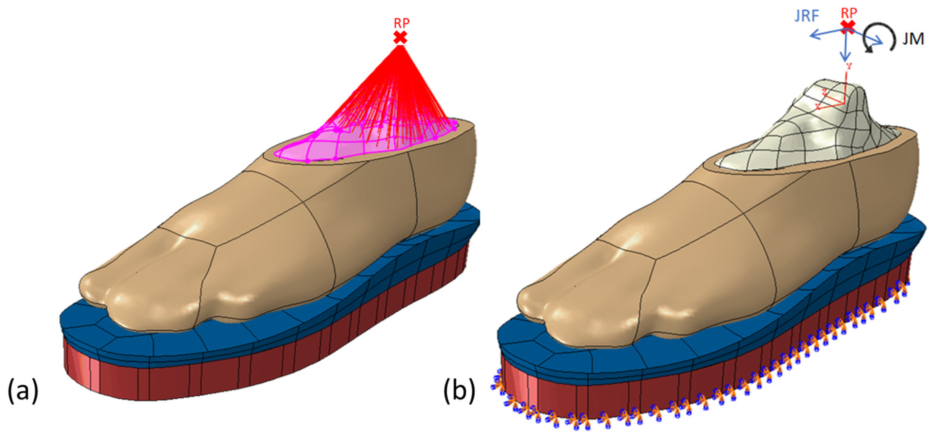
2.4.4. Boundary and Loading Condition

The lower surface of the shoe sole was fixed in all directions throughout the simulation. As the forces were transmitted from the tibia and fibula to the talus at the ankle joint, the ankle reaction forces and moments were also applied to the surface of the talus in the FE model [57]. For this purpose, a reference point was created and coupled to the talus surface using a kinematic coupling (Figure 5a). Between the foot and insole, normal contact was assumed to be hard and tangential contact was defined with a coefficient of friction of 0.5 [55]. The insole was tied to the shoe sole, allowing no relative movements.

In the first analysis step, a displacement of 10 mm in the negative y-direction (vertical direction) of the calcaneus coordinate system was applied to the talus via the reference point (Figure 5b), while the remaining directions (translation and rotation) were constrained. In this manner, the first contact between the surface of the foot and the insole could be found. In the second step, joint reaction forces and dorsal flexion moment calculated within the musculoskeletal multibody simulation were applied to the talus via the reference point. At the same time, just the rotation around the x-axis was constrained, while the remaining directions were not. All boundary conditions and forces were applied with respect to the implemented calcaneus coordinate system from Wu et al. [48]. The exact values of the forces and dorsal flexion moment used can be taken from

Table 3. Boundary conditions of the FE model; i.e., dorsiflexion moment (JM) and joint reaction forces (JRF) of the ankle at the two-time points of the first high point and low point of the vertical ground reaction force calculated in the musculoskeletal multibody simulation.

	High Point Ground Reaction Force	Low Point Ground Reaction Force
JM—Dorsiflexion [Nmm]	24,002.00	53,192.00
JRF—Medio (−)/Lateral (+) [N]	−38.20	2.28
JRF—Anterior (−)/Posterior (+) [N]	86.42	−24.19
JRF—Proximal (−)/Distal (+) [N]	704.68	577.78

.

2.4.5. Validation

For validation, the calculated and experimentally recorded plantar peak pressure values and plantar pressure distributions were compared at the time of the vertical ground reaction force’s first high point and low point. Since the experimental plantar pressure data were synchronously recorded with the 3D gait analysis, a direct comparison between experimental and simulated values was possible.

2.4.6. Parameter Analysis

To adapt the stiffness of the individual insole, soft insole plugs were inserted at the points where high plantar pressure values occurred. For diabetes-adapted insoles, it is recommended to reduce plantar peak pressures above 200 kPa experimentally measured with a sensor size of 2 cm² to reduce the incidence of ulcers [13,17]. Since FE analysis calculates the nodal contact pressure, these values were chosen to adjust the stiffness of the insole. As the modelled subject represents a healthy foot, areas above plantar pressures of 100 kPa were partitioned for illustration. Soft insert plugs have shown plantar pressure reduction and have the advantage of keeping the already fitted shape unchanged in the process [24,25,29,58]. The round or oval areas were chosen to be slightly larger than the areas of high pressure to avoid an edge effect [25,58,59]. For simplification, lower stiffness was assigned to these areas by reducing Young’s modulus. Thus, different elastic moduli were tested in a parameter analysis: 1.5 MPa, 1.0 MPa, and 0.5 MPa. The later additively manufactured insole material and infill should be changed in order to comply with Young’s modulus.

3. Results

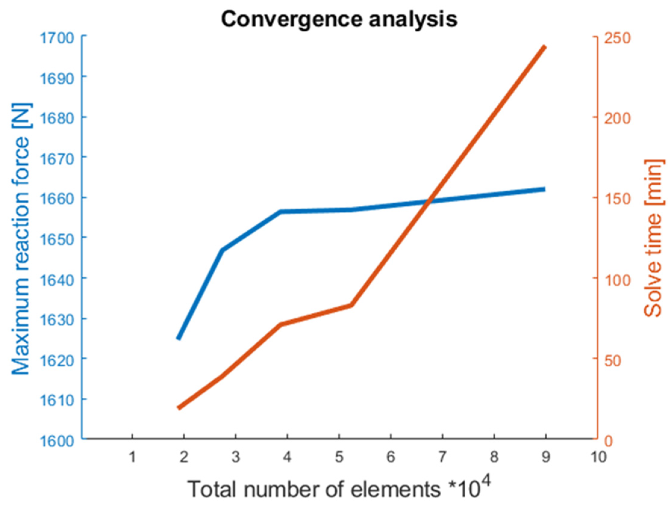
3.1. Convergence Analysis

In

Table 4. Results of the convergence analysis of the different mesh densities.

Mesh	Element Size [mm]	Total Number of Elements	Total Number of Nodes	Maximal Reaction Force [N]	Percentage Deviation to the Finest Mesh [%]	Computation Time [min]
1	9	18,696	23,144	1624.7	−1.9	19
2	8	27,272	33,997	1646.8	−0.9	39
3	7	38,553	47,035	1656.4	−0.3	71
4	6	51,702	60,775	1656.9	−0.3	83
5	5	89,761	104,405	1662.0	-	244

and Figure 6, the results of the convergence analysis are given. The maximum reaction force converged toward a value of 1662 N. The coarsest mesh, mesh number 1, had the highest percentage deviation of −1.9%. As the mesh density increased, the percentage deviation from the value of the finest mesh decreased. In general, the percentage deviation was low for all meshes. As the number of elements increased, an exponential increase in computation solving time becomes apparent.

In terms of the plantar pressure distribution, it was seen that as the number of elements increased, the plantar pressure distribution approached a specific pressure distribution pattern (Figure 7).

Accordingly, in the convergence analysis, a suitable mesh for the FE model was found. The maximum reaction force, as the primary evaluation criterion, showed a desired converging result, with a deviation of less than three percent for all meshes. The mesh with 51,702 elements and 60,775 integration points was chosen because an even finer mesh no longer showed considerable differences in the plantar pressure distribution. The calculation times of 83 min were assumed to be acceptable, with respect to the performance of other parameter studies to adjust the stiffness of the insole.

3.2. Experimental Validation of the FE Model

Figure 8 shows the experimental plantar pressure values recorded by means of the pressure measurement insoles (Pedar), as a sensor view and as an isobar view (Figure 8a), as well as the numerically determined plantar pressure distribution at the time of the first high point of the vertical ground reaction force from the FE model (Figure 8b). In both cases, the highest plantar pressure was located in the rearfoot area centred on the heel. The deviation between the peak pressure value of the simulation and the experimentally determined peak pressure value amounted to 234 kPa. While, in the experimental case, the plantar pressure was mainly distributed in the heel; the simulated plantar pressure extended even further into the midfoot region.

Figure 9 shows the experimental and numerical pressure distributions at the time of the low point of the vertical ground reaction force. In the experimental case (Figure 9a), the maximum plantar pressure is in the toe region, whereas in the simulated case (Figure 9b), the maximum plantar pressure is in the lateral forefoot region. Here, the deviation of the numerically calculated peak value from the experimental value is only 30 kPa. While the pressure measurement insoles recorded little plantar pressure load in the midfoot region; in the simulated case, plantar pressure loads mainly occur in the lateral midfoot region.

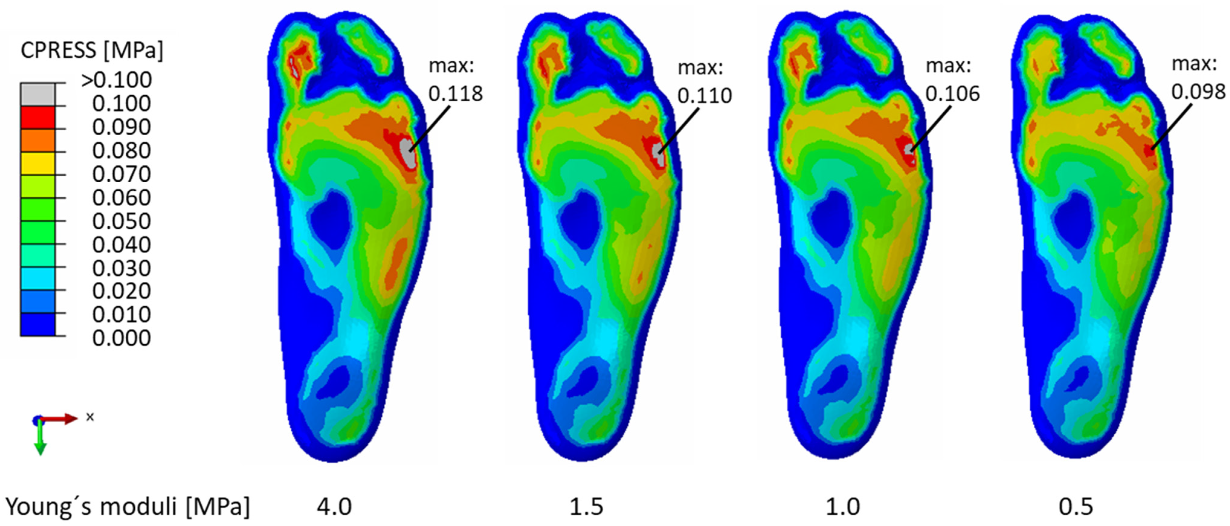
3.3. Parameter Analysis

According to the plantar pressure distribution of the FE model, plantar pressure values of more than 100 kPa were calculated on the insole in the heel area and lateral midfoot at the time of the first high point, and in the toe area and lateral forefoot area at the time of the low point of the ground reaction force. Therefore, the insole was partitioned in these areas. Figure 10 shows the plantar pressure distribution of the left insole and their corresponding partitioning.

Figure 11 and Figure 12 show the results of the plantar pressure distribution as a function of the Young’s moduli 1.5 MPa, 1.0 MPa, and 0.5 MPa used for the adapted insole. In each case, the pressure distribution without adjustment of the insole stiffness is taken as the reference. The respective percentage reductions in peak pressure are summarized in

Table 5. Percentage reduction of the peak plantar pressure at the heel and lateral midfoot at the time of the first high point of the vertical ground reaction force, as well as in the lateral forefoot and toe at the time of the low point of the vertical ground reaction force depending on the Young’s moduli 0.5 MPa, 1.0 MPa, and 1.5 MPa of the corresponding soft insole used compared to the peak plantar pressure without stiffness adjustment of the insole.

	Percentage Reduction in Peak Plantar Pressure [%]
Area	1.5 MPa	1.0 MPa	0.5 MPa
Heel	−8.16	−13.01	−22.96
Lateral Midfoot	−4.44	−8.15	−16.30
Lateral Forefoot	−6.78	−10.17	−16.95
Toe	−11.30	−17.39	−26.09

.

The use of a Young’s modulus of 0.5 MPa resulted in the largest peak pressure reduction in all areas. As shown in Figure 11, there was a slight redistribution of pressure towards the medial midfoot region. In the lateral forefoot and toe regions, a reduction in peak plantar pressure of 16.95% and 26.09% at the time of the low point of the vertical ground reaction force was achieved at a Young’s modulus of 0.5 MPa. The peak pressure here was less than 0.1 MPa. Figure 12 shows that the pressure mainly shifted to the medial forefoot region with decreasing Young´s modulus.

4. Discussion

In this study, a method was developed to adapt the stiffness of an individual insole using the FE method with boundary conditions from a musculoskeletal multibody model during walking. Afterwards, the insole was manufactured by means of additive manufacturing processes. It has to be noted that a FE model is always a simplification and, therefore, only an approximation of reality. The foot is a complex structure consisting of numerous ligaments, joints, and musculature. The more detailed the model is, the more computational time is required and the more difficult it becomes to achieve convergence [60]. Therefore, to make the FE model as efficient as possible, in this work, only the most important structures, the foot skeleton and the foot surface, were used [28,61]. However, this is one limitation of the present study.

Recommendations exist to adapt insoles based on plantar pressure distribution during gait [13,17]. Therefore, a static analysis of two-time points of gait was simulated; i.e., the early and late middle stance phases were used. However, it should be noted that the time points chosen for the FE model do not correspond to the phases that exhibit the highest peak plantar pressures. These occur at the time of the heel strike and during the push-off phase [62]. However, this would require MRI scans of two different foot or foot skeletal positions if relative motions of bone structures are not considered, as in this FE model. In contrast, the foot is flat on the insole during the early and late mid-stance phase, which is why these time points were chosen.

By simplifying the foot skeletal geometry, the cushioning properties of the foot, through arch, ligaments, as well as joints, were not considered. The neglect of the relative motions of the bones has also been described in some other studies and may be the cause of some of the observed deviations with respect to their validation [34,63,64]. The reason for this is the challenging modelling of joints in FE analysis [22]. Furthermore, most studies have equally relied on MRI or CT data to obtain patient-specific foot skeletal geometries. However, these procedures are very costly or, in the case of CT, involve radiation exposure. In addition, reconstruction of geometries from MRI cross-sectional images is usually difficult and often has to be manually conducted, which increases the workload. The dependence on these imaging techniques is a major problem, which has been previously addressed [22,23,65]. Therefore, attempts have been started to generate individualized geometries using ultrasound images [61,66]. Another conceivable option would be to use a CAD programme to customize a standardized skeleton.

The contact between the bone and the soft tissue was neglected by merging and meshing them together. This simplification has also been used in other studies, since with a larger number of contacts, the computational time increases [29,67]. However, Bocanegra et al. [60] showed that the use of a common mesh has little effect on the results of plantar pressure distribution when the soft tissue is assigned hyperelastic material properties. Therefore, this simplification will only have a minor impact on our results.

The material assignment for the plantar tissue was carried out with a hyperelastic material for the reasons mentioned before. For this purpose, the material properties according to Chen et al. [56] were used, which were also used for a subject with healthy plantar tissue and a similar age to that of the subject in this study. It was also experimentally shown that the plantar tissue has a hyperelastic property [55]. Furthermore, the normally multilayered soft tissue was defined as a homogeneous structure. However, according to Petre et al. [68], this may have had little effect on plantar pressure in the FE simulation, although stresses in the soft tissue cannot be used for investigation in this case. A further material simplification was made for the bone tissue. Only one linear elastic material was chosen for the normally inhomogeneous bone consisting of cancellous and cortical bone. This simplification was used because material assignment for an inhomogeneous bone structure is a time-consuming procedure in the FE method [69]. The linear elastic bone property introduced by Nakamura et al. [52] used in this FE model has also been applied in most studies [27,35,36,56,70]. However, it should be noted that the characteristics of the tissue and also of the bone vary from individual to individual. Here, age or diseases of the foot also have an influence [71]. People suffering from diabetes in particular usually have stiffer plantar tissue, which additionally increases the occurrence of ulcers [72]. This must be taken into account when fitting diabetes-adapted insoles.

The additively manufactured insole was initially considered homogeneous in the FE model as it was made from one material, one infill, and one filler structure. However, additively manufactured components generally exhibit inhomogeneous and anisotropic properties [73]. Furthermore, the structural material of the insole was additionally wrapped with an edge, top, and bottom layer. To prevent the influence of the envelope layers, the insoles could be designed without an envelope, as done by Tang et al. [34].

The friction coefficient between the insole and the foot was chosen as 0.5. In the literature, different coefficients of friction have been defined for the contact between the insole and foot, which range from 0.3 [34] to 0.6 [35]. Therefore, the influence of the friction coefficient on the plantar pressure was examined in a sensitivity study. It was shown that friction coefficients showed a minor influence on the pressure distribution pattern and the maximum pressure values. These results are in agreement with the sensitivity analysis according to Goske et al. [26]. Due to this, the friction coefficient of 0.5 used in this work was not considered further in the result analysis.

In order to enable the calculation of the individual plantar pressure values, subject-specific boundary conditions were used for the FE model [74]. In most studies, elaborate muscle forces have been applied via muscle connectors and/or ground reaction forces. To generate the FE model as efficiently as possible in this study, subject-specific ankle reaction forces and moments were used. For this purpose, data from the subject’s 3D gait analysis was imported into a musculoskeletal multi-body model. The results of the musculoskeletal model showed good agreement with data in the literature [75]. Since only five markers were placed on each foot, inaccuracies may have occurred in the calculation. More markers could be used to record the movement of the foot more accurate in further studies [76]. It should also be noted that shoes dedicated to people suffering from diabetes were worn during the measurements. Thus, the exact movements of the foot within the shoe could only be approximated. In the study by Peng et al. [32], a 3D gait analysis was performed with the insoles worn in sandals so that the markers could be directly applied to the skin. However, in this case, the plantar pressure distributions in the diabetic shoe could not have been used to adjust the stiffness of the insole as recommended [13,17]. To detect the timing of the early and mid-stance phases, the first high point and low point of the vertical ground reaction force were used. The early mean stance phase was 30.5% and the late mean stance phase was 51.2% of the stance phase. These values are consistent with those in the literature [62], demonstrating that the data of our FE simulation are realistic.

When transferring the boundary conditions from the multibody simulation to the FE method, inaccuracies may have occurred; e.g., due to inaccuracies in the implementation of the heel coordinate system in the FE method. In order to minimize this in the future or to further reduce the workload, a coupling of the musculoskeletal multibody modelling with the FE method may be performed. This could also simplify dynamic FE analyses [77,78,79].

The validation showed that the percentage deviations between the experimental and simulated plantar peak pressure values are high, but the localization of the plantar pressure distribution is similar. However, the different resolutions between the experimental and simulated pressure measurement images must be taken into account. While Pedar pressure measurement insoles capture pressure within approximately 2 cm² areas, the FE method calculates nodal contact pressure [23,35,63,66]. A crucial reason for the discrepancies may be due to the neglect of the relative motion of the bones. In addition, the damping property of joints and ligaments was excluded due to the fusion of all bones. Because of the discrepancies between the experimental and simulated plantar pressure distributions, the prediction of absolute changes in plantar pressure distribution due to a change in the stiffness of the insole using the FE model is not fully possible. However, it is assumed that a qualitative statement can be made about the influence of a change in the insole material on the plantar pressure distribution. Therefore, the computer-based method can be used to identify the location of high plantar pressure values in patients with diabetic foot, and it is assumed that a reduction in Young’s modulus at these locations leads to a reduction in the plantar pressures using, accordingly, 3D-printed insoles.

By means of a parameter analysis, the stiffness of the individual insole should be adjusted at local points where high plantar pressure values are present. This is because both experimental and numerical studies show a positive effect of local soft plugs on plantar pressure redistribution. Furthermore, Eckardt and Lobmann [80] found that placement of insoles after plantar pressures has a better effect on peak pressure reduction than placement after bony structures. In this work, the elastic modulus of 0.5 MPa, 1.0 MPa, and 1.5 MPa was investigated, which corresponds to a Shore A hardness of approximately 9, 20, and 29, respectively, according to the conversion formula of Kunz and Studer [81]. Due to the high resolution of the simulated plantar pressure distribution, the corresponding local areas on the insole could be easily identified, partitioned, and materials assigned, which is another advantage of the FE method over manual stiffness adjustment using experimental data. The results of the FE method show that the greatest plantar peak pressure reduction can be achieved using the elastic modulus of 0.5 MPa. Here, percentage reductions between 16% and 26% were achieved in the different areas. Erdemir et al. [25] found that too small diameters can produce so-called edge effects, which means a high pressure at the edge of the partitioning. In the next step, further insole modifications could be carried out to minimize the still relatively high peak pressure in the heel area. Furthermore, it has to be verified which infill and material of the insole are additively manufactured to match the adjusted elastic modulus.

The future goal is to produce patient-specific 3D-printed insoles that can be made available in a timely manner. It should enable technicians who lack the relevant in-depth experience to manufacture insoles for diabetic patients, including proof of function. For this purpose, it is necessary to coordinate the requirements for the insoles with the biomechanical requirements, as well as the manufacturing issues, in such a way that the insoles can be made available to the patient in a cost-effective and timely manner.

5. Conclusions

By means of the presented computer-based method, it is possible to adjust the stiffness of an individually 3D-printed insole for patients with diabetic foot syndrome in order to reduce plantar pressure with a parametric FE analysis. Moreover, this efficient method allows the adjustment of the stiffness of insoles during walking according to the recommendations of the International Working Group of the Diabetic Foot [13]. It was found that the absolute deviations between the experimental and simulated plantar peak pressures were high, but the localization of the plantar pressure distribution was similar. Therefore, a qualitative comparison of additively manufactured insole materials on the plantar pressure distribution is assumed to be suitable. In the future, further simplifications and automation should be carried out.

References

1. International Diabetes Federation. IDF Diabetes Atlas, 10th ed. 2021. Available online: https://diabetesatlas.org/data/en/country/77/de.html (accessed on 2 August 2021).
2. Zhang, Y.; Lazzarini, P.A.; McPhail, S.M.; van Netten, J.J.; Armstrong, D.G.; Pacella, R.E. Global Disability Burdens of Diabetes-Related Lower-Extremity Complications in 1990 and 2016. Diabetes Care 2020, 43, 964–974. [Google Scholar] [CrossRef]
3. Armstrong, D.G.; Boulton, A.J.M.; Bus, S.A. Diabetic Foot Ulcers and Their Recurrence. N. Engl. J. Med. 2017, 376, 2367–2375. [Google Scholar] [CrossRef] [PubMed]
4. Morbach, S.; Müller, E.; Reike, H.; Risse, A.; Rümenapf, G.; Spraul, M. Diabetic Foot Syndrome. Exp. Clin. Endocrinol. Diabetes 2014, 122, 416–424. [Google Scholar] [CrossRef] [PubMed] [Green Version]
5. Cheng, Q.; Lazzarini, P.A.; Gibb, M.; Derhy, P.H.; Kinnear, E.M.; Burn, E.; Graves, N.; Norman, R.E. A cost-effectiveness analysis of optimal care for diabetic foot ulcers in Australia. Int. Wound J. 2016, 14, 616–628. [Google Scholar] [CrossRef]
6. Kröger, K.; Berg, C.; Santosa, F.; Malyar, N.; Reinecke, H. Lower Limb Amputation in Germany. Dtsch. Arztebl. Int. 2017, 114, 130–136. [Google Scholar] [CrossRef] [Green Version]
7. Norman, G.; Westby, M.J.; Vedhara, K.; Game, F.; Cullum, N.A. Effectiveness of psychosocial interventions for the prevention and treatment of foot ulcers in people with diabetes: A systematic review. Diabet. Med. 2020, 37, 1256–1265. [Google Scholar] [CrossRef]
8. Armstrong, D.G.; Swerdlow, M.A.; Armstrong, A.A.; Conte, M.S.; Padula, W.V.; Bus, S.A. Five year mortality and direct costs of care for people with diabetic foot complications are comparable to cancer. J. Foot Ankle Res. 2020, 13, 16. [Google Scholar] [CrossRef] [Green Version]
9. Lazzarini, P.A.; Pacella, R.E.; Armstrong, D.G.; Van Netten, J.J. Diabetes-related lower-extremity complications are a leading cause of the global burden of disability. Diabet. Med. 2018, 35, 1297–1299. [Google Scholar] [CrossRef] [PubMed]
10. Singh, N.; Armstrong, D.G.; Lipsky, B.A. Preventing Foot Ulcers in Patients with Diabetes. JAMA 2005, 293, 217–228. [Google Scholar] [CrossRef]
11. Bus, S.A. Priorities in offloading the diabetic foot. Diabetes Metab. Res. Rev. 2012, 28, 54–59. [Google Scholar] [CrossRef]
12. Bus, S.A.; van Deursen, R.; Armstrong, D.G.; Lewis, J.E.A.; Caravaggi, C.F.; Cavanagh, P.R.; on behalf of the International Working Group on the Diabetic Foot (IWGDF). Footwear and offloading interventions to prevent and heal foot ulcers and reduce plantar pressure in patients with diabetes: A systematic review. Diabetes Metab. Res. Rev. 2016, 32, 99–118. [Google Scholar] [CrossRef] [Green Version]
13. Bus, S.A.; Lavery, L.A.; Monteiro-Soares, M.; Rasmussen, A.; Raspovic, A.; Sacco, I.C.; van Netten, J.J.; on behalf of the International Working Group on the Diabetic Foot. Guidelines on the prevention of foot ulcers in persons with diabetes (IWGDF 2019 update). Diabetes Metab. Res. Rev. 2020, 36, e3269. [Google Scholar] [CrossRef] [PubMed] [Green Version]
14. Collings, R.; Freeman, J.; Latour, J.M.; Paton, J. Footwear and insole design features for offloading the diabetic at risk foot—A systematic review and meta-analyses. Endocrinol. Diabetes Metab. 2020, 4, e00132. [Google Scholar] [CrossRef] [Green Version]
15. Jeffcoate, W.J.; Harding, K.G. Diabetic foot ulcers. Lancet 2003, 361, 1545–1551. [Google Scholar] [CrossRef]
16. Rizzo, L.; Tedeschi, A.; Fallani, E.; Coppelli, A.; Vallini, V.; Iacopi, E.; Piaggesi, A. Custom-Made Orthesis and Shoes in a Structured Follow-Up Program Reduces the Incidence of Neuropathic Ulcers in High-Risk Diabetic Foot Patients. Int. J. Low. Extrem. Wounds 2012, 11, 59–64. [Google Scholar] [CrossRef] [PubMed]
17. Schaper, N.C.; Van Netten, J.J.; Apelqvist, J.; Bus, S.A.; Hinchliffe, R.J.; Lipsky, B.A.; IWGDF Editorial Board. Practical Guidelines on the prevention and management of diabetic foot disease (IWGDF 2019 update). Diabetes Metab. Res. Rev. 2020, 36 (Suppl. S1), e3266. [Google Scholar] [CrossRef] [PubMed] [Green Version]
18. Van Netten, J.J.; Price, P.E.; Lavery, L.A.; Monteiro-Soares, M.; Rasmussen, A.; Jubiz, Y.; Bus, S.A.; on behalf of the International Working Group on the Diabetic Foot (IWGDF). Prevention of foot ulcers in the at-risk patient with diabetes: A systematic review. Diabetes Metab. Res. Rev. 2016, 32, 84–98. [Google Scholar] [CrossRef] [Green Version]
19. Davia-Aracil, M.; Hinojo-Pérez, J.J.; Jimeno-Morenilla, A.; Mora-Mora, H. 3D printing of functional anatomical insoles. Comput. Ind. 2018, 95, 38–53. [Google Scholar] [CrossRef] [Green Version]
20. Hellstrand, S.; Sundberg, L.; Karlsson, J.; Zügner, R.; Tranberg, R.; Tang, U.H. Measuring sustainability in healthcare: An analysis of two systems providing insoles to patients with diabetes. Environ. Dev. Sustain. 2020, 23, 6987–7001. [Google Scholar] [CrossRef]
21. Paton, J.S.; Stenhouse, E.A.; Bruce, G.; Zahra, D.; Jones, R.B. A comparison of customised and prefabricated insoles to reduce risk factors for neuropathic diabetic foot ulceration: A participant-blinded randomised controlled trial. J. Foot Ankle Res. 2012, 5, 31. [Google Scholar] [CrossRef] [Green Version]
22. Behforootan, S.; Chatzistergos, P.; Naemi, R.; Chockalingam, N. Finite element modelling of the foot for clinical application: A systematic review. Med. Eng. Phys. 2017, 39, 1–11. [Google Scholar] [CrossRef] [PubMed]
23. Telfer, S.; Erdemir, A.; Woodburn, J.; Cavanagh, P.R. What Has Finite Element Analysis Taught Us about Diabetic Foot Disease and Its Management? A Systematic Review. PLoS ONE 2014, 9, e109994. [Google Scholar] [CrossRef]
24. Actis, R.L.; Ventura, L.B.; Lott, D.J.; Smith, K.E.; Commean, P.K.; Hastings, M.; Mueller, M.J. Multi-plug insole design to reduce peak plantar pressure on the diabetic foot during walking. Med. Biol. Eng. Comput. 2008, 46, 363–371. [Google Scholar] [CrossRef] [PubMed]
25. Erdemir, A.; Saucerman, J.J.; Lemmon, D.; Loppnow, B.; Turso, B.; Ulbrecht, J.S.; Cavanagh, P.R. Local plantar pressure relief in therapeutic footwear: Design guidelines from finite element models. J. Biomech. 2005, 38, 1798–1806. [Google Scholar] [CrossRef]
26. Goske, S.; Erdemir, A.; Petre, M.; Budhabhatti, S.; Cavanagh, P.R. Reduction of plantar heel pressures: Insole design using finite element analysis. J. Biomech. 2006, 39, 2363–2370. [Google Scholar] [CrossRef] [PubMed]
27. Cheung, J.T.-M.; Zhang, M. Parametric design of pressure-relieving foot orthosis using statistics-based finite element method. Med. Eng. Phys. 2008, 30, 269–277. [Google Scholar] [CrossRef]
28. Ghazali, M.; Ren, X.; Rajabi, A.; Zamri, W.; Mustafah, N.M.; Ni, J. Finite Element Analysis of Cushioned Diabetic Footwear Using Ethylene Vinyl Acetate Polymer. Polymers 2021, 13, 2261. [Google Scholar] [CrossRef] [PubMed]
29. Gu, Y.D.; Li, J.S.; Lake, M.J.; Zeng, Y.J.; Ren, J.; Li, Z.-Y. Image-based midsole insert design and the material effects on heel plantar pressure distribution during simulated walking loads. Comput. Methods Biomech. Biomed. Eng. 2011, 14, 747–753. [Google Scholar] [CrossRef]
30. Gu, Y.D.; Ren, X.J.; Li, J.S.; Lake, M.J.; Zhang, Q.Y.; Zeng, Y.J. Computer simulation of stress distribution in the metatarsals at different inversion landing angles using the finite element method. Int. Orthop. 2010, 34, 669–676. [Google Scholar] [CrossRef] [Green Version]
31. Nouman, M.; Dissaneewate, T.; Chong, D.; Chatpun, S. Effects of Custom-Made Insole Materials on Frictional Stress and Contact Pressure in Diabetic Foot with Neuropathy: Results from a Finite Element Analysis. Appl. Sci. 2021, 11, 3412. [Google Scholar] [CrossRef]
32. Peng, Y.; Wong, D.W.-C.; Chen, T.L.-W.; Wang, Y.; Zhang, G.; Yan, F.; Zhang, M. Influence of arch support heights on the internal foot mechanics of flatfoot during walking: A muscle-driven finite element analysis. Comput. Biol. Med. 2021, 132, 104355. [Google Scholar] [CrossRef] [PubMed]
33. Su, S.; Mo, Z.; Guo, J.; Fan, Y. The Effect of Arch Height and Material Hardness of Personalized Insole on Correction and Tissues of Flatfoot. J. Healthc. Eng. 2017, 2017, 8614341. [Google Scholar] [CrossRef] [Green Version]
34. Tang, L.; Wang, L.; Bao, W.; Zhu, S.; Li, D.; Zhao, N.; Liu, C. Functional gradient structural design of customized diabetic insoles. J. Mech. Behav. Biomed. Mater. 2019, 94, 279–287. [Google Scholar] [CrossRef]
35. Cheung, J.T.-M.; Zhang, M. A 3-dimensional finite element model of the human foot and ankle for insole design. Arch. Phys. Med. Rehabil. 2005, 86, 353–358. [Google Scholar] [CrossRef]
36. Akrami, M.; Qian, Z.; Zou, Z.; Howard, D.; Nester, C.J.; Ren, L. Subject-specific finite element modelling of the human foot complex during walking: Sensitivity analysis of material properties, boundary and loading conditions. Biomech. Model. Mechanobiol. 2018, 17, 559–576. [Google Scholar] [CrossRef] [PubMed] [Green Version]
37. Scarton, A.; Guiotto, A.; Malaquias, T.; Spolaor, F.; Sinigaglia, G.; Cobelli, C.; Jonkers, I.; Sawacha, Z. A methodological framework for detecting ulcers’ risk in diabetic foot subjects by combining gait analysis, a new musculoskeletal foot model and a foot finite element model. Gait Posture 2018, 60, 279–285. [Google Scholar] [CrossRef]
38. Morales-Orcajo, E.; Souza, T.R.; Bayod, J.; Casas, E.B.D.L. Non-linear finite element model to assess the effect of tendon forces on the foot-ankle complex. Med. Eng. Phys. 2017, 49, 71–78. [Google Scholar] [CrossRef]
39. Tsung, B.Y.S.; Zhang, M.; Mak, A.F.T.; Wong, M.W.N. Effectiveness of insoles on plantar pressure redistribution. J. Rehabil. Res. Dev. 2004, 41, 767–774. [Google Scholar] [CrossRef] [Green Version]
40. Ren, X.; Lutter, C.; Kebbach, M.; Bruhn, S.; Bader, R.; Tischer, T. Lower extremity joint compensatory effects during the first recovery step following slipping and stumbling perturbations in young and older subjects. BMC Geriatr. 2022, 22, 656. [Google Scholar] [CrossRef]
41. Ren, X.; Lutter, C.; Kebbach, M.; Bruhn, S.; Yang, Q.; Bader, R.; Tischer, T. Compensatory Responses During Slip-Induced Perturbation in Patients with Knee Osteoarthritis Compared with Healthy Older Adults: An Increased Risk of Falls? Front. Bioeng. Biotechnol. 2022, 10, 893840. [Google Scholar] [CrossRef] [PubMed]
42. Van den Bogert, A.J.; Geijtenbeek, T.; Even-Zohar, O.; Steenbrink, F.; Hardin, E.C. A real-time system for biomechanical analysis of human movement and muscle function. Med. Biol. Eng. Comput. 2013, 51, 1069–1077. [Google Scholar] [CrossRef] [PubMed] [Green Version]
43. Carbone, V.; Fluit, R.; Pellikaan, P.; van der Krogt, M.M.; Janssen, D.; Damsgaard, M.; Vigneron, L.; Feilkas, T.; Koopman, H.F.J.M.; Verdonschot, N. TLEM 2.0—A comprehensive musculoskeletal geometry dataset for subject-specific modeling of lower extremity. J. Biomech. 2015, 48, 734–741. [Google Scholar] [CrossRef] [PubMed] [Green Version]
44. Damsgaard, M.; Rasmussen, J.; Christensen, S.T.; Surma, E.; de Zee, M. Analysis of musculoskeletal systems in the AnyBody Modeling System. Simul. Model. Pract. Theory 2006, 14, 1100–1111. [Google Scholar] [CrossRef]
45. Andersen, M.S. Introduction to musculoskeletal modelling. In Computational Modelling of Biomechanics and Biotribology in the Musculoskeletal System; Elsevier: Amsterdam, The Netherlands, 2021; pp. 41–80. [Google Scholar]
46. Qian, Z.; Ren, L.; Ding, Y.; Hutchinson, J.R.; Ren, L. A Dynamic Finite Element Analysis of Human Foot Complex in the Sagittal Plane during Level Walking. PLoS ONE 2013, 8, e79424. [Google Scholar] [CrossRef] [PubMed] [Green Version]
47. Ren, L.; Jones, R.K.; Howard, D. Whole body inverse dynamics over a complete gait cycle based only on measured kinematics. J. Biomech. 2008, 41, 2750–2759. [Google Scholar] [CrossRef]
48. Wu, G.; Siegler, S.; Allard, P.; Kirtley, C.; Leardini, A.; Rosenbaum, D.; Whittle, M.; D’Lima, D.D.; Cristofolini, L.; Witte, H.; et al. ISB recommendation on definitions of joint coordinate system of various joints for the reporting of human joint motion—Part I: Ankle, hip, and spine. J. Biomech. 2002, 35, 543–548. [Google Scholar] [CrossRef]
49. Kluess, D.; Souffrant, R.; Mittelmeier, W.; Wree, A.; Schmitz, K.-P.; Bader, R. A convenient approach for finite-element-analyses of orthopaedic implants in bone contact: Modeling and experimental validation. Comput. Methods Programs Biomed. 2009, 95, 23–30. [Google Scholar] [CrossRef]
50. ASTM D 3574-17; D20 Committee. Standard Test Methods for Flexible Cellular Materials Slab, Bonded, and Molded Urethane Foams. ASTM International: West Conshohocken, PA, USA, 2017. [Google Scholar]
51. Häfele, P.; Issler, L.; Ruoß, H. Festigkeitslehre—Grundlagen, 2nd ed.; Springer: Berlin/Heidelberg, Germany, 2003. [Google Scholar]
52. Nakamura, S.; Crowninshield, R.D.; Cooper, R.R. An Analysis of Soft Tissue Loading in the Foot—A Preliminary Report; Bulletin of Prosthetics Research: Washington, DC, USA, 1981. [Google Scholar]
53. Xu, Y.-X.; Juang, J.-Y. Measurement of Nonlinear Poisson’s Ratio of Thermoplastic Polyurethanes under Cyclic Softening Using 2D Digital Image Correlation. Polymers 2021, 13, 1498. [Google Scholar] [CrossRef]
54. Lewis, G. Finite element analysis of a model of a therapeutic shoe: Effect of material selection for the outsole. Bio-Med. Mater. Eng. 2003, 13, 75–81. [Google Scholar]
55. Lemmon, D.; Shiang, T.; Hashmi, A.; Ulbrecht, J.S.; Cavanagh, P.R. The effect of insoles in therapeutic footwear—A finite element approach. J. Biomech. 1997, 30, 615–620. [Google Scholar] [CrossRef]
56. Chen, W.-M.; Lee, T.; Lee, P.V.S.; Lee, J.W.; Lee, S.-J. Effects of internal stress concentrations in plantar soft-tissue—A preliminary three-dimensional finite element analysis. Med. Eng. Phys. 2010, 32, 324–331. [Google Scholar] [CrossRef]
57. Faller, A.; Schünke, M.; Schünke, G. Der Körper des Menschen: Einführung in Bau und Funktion; 4 Poster mit Übersichten Skelett, Gefäße, Nerven, Muskeln, 16., überarb. Aufl.; Georg Thieme Verlag KG: Stuttgart, Germany, 2012. [Google Scholar]
58. Mandolini, M.; Brunzini, A.; Manieri, S.; Germani, M. Foot plantar pressure offloading: How to select the right material for a custom-made insole. In DS 87-1 Proceedings of the 21st International Conference on Engineering Design (ICED 17) Vol 1: Resource Sensitive Design, Design Research Applications and Case Studies, Vancouver, BC, Canada, 21–25 August 2017; Universitŕ Politecnica delle Marche: Ancona, Italy, 2017; pp. 469–478. [Google Scholar]
59. Bus, S.A.; Zwaferink, J.B.; Dahmen, R.; Busch-Westbroek, T. State of the art design protocol for custom made footwear for people with diabetes and peripheral neuropathy. Diabetes Metab. Res. Rev. 2020, 36, e3237. [Google Scholar] [CrossRef]
60. Bocanegra, M.; López, J.; Vidal-Lesso, A.; Tobar, A.; Vallejo, R. Numerical Assessment of the Structural Effects of Relative Sliding between Tissues in a Finite Element Model of the Foot. Mathematics 2021, 9, 1719. [Google Scholar] [CrossRef]
61. Telfer, S.; Erdemir, A.; Woodburn, J.; Cavanagh, P.R. Simplified versus geometrically accurate models of forefoot anatomy to predict plantar pressures: A finite element study. J. Biomech. 2016, 49, 289–294. [Google Scholar] [CrossRef]
62. Perry, J. Ganganalyse: Norm und Pathologie des Gehens, 1st ed.; Urban & Fischer: München, Germany, 2003. [Google Scholar]
63. Dai, X.-Q.; Li, Y.; Zhang, M.; Cheung, J.T.-M. Effect of sock on biomechanical responses of foot during walking. Clin. Biomech. 2006, 21, 314–321. [Google Scholar] [CrossRef]
64. Guiotto, A.; Sawacha, Z.; Guarneri, G.; Avogaro, A.; Cobelli, C. 3D finite element model of the diabetic neuropathic foot: A gait analysis driven approach. J. Biomech. 2014, 47, 3064–3071. [Google Scholar] [CrossRef] [PubMed]
65. Wang, Y.; Wong, D.W.-C.; Zhang, M. Computational Models of the Foot and Ankle for Pathomechanics and Clinical Applications: A Review. Ann. Biomed. Eng. 2016, 44, 213–221. [Google Scholar] [CrossRef]
66. Spirka, T.A.; Erdemir, A.; Spaulding, S.E.; Yamane, A.; Telfer, S.; Cavanagh, P.R. Simple finite element models for use in the design of therapeutic footwear. J. Biomech. 2014, 47, 2948–2955. [Google Scholar] [CrossRef] [Green Version]
67. Natali, A.N.; Forestiero, A.; Carniel, E.L.; Pavan, P.G.; Dal Zovo, C. Investigation of foot plantar pressure: Experimental and numerical analysis. Med. Biol. Eng. Comput. 2010, 48, 1167–1174. [Google Scholar] [CrossRef] [PubMed]
68. Petre, M.; Erdemir, A.; Panoskaltsis, V.P.; Spirka, T.A.; Cavanagh, P.R. Optimization of Nonlinear Hyperelastic Coefficients for Foot Tissues Using a Magnetic Resonance Imaging Deformation Experiment. J. Biomech. Eng. 2013, 135, 61001–61012. [Google Scholar] [CrossRef] [Green Version]
69. Li, J.; Chen, Z.; Jin, Z. (Eds.) Computational Modelling of Biomechanics and Biotribology in the Musculoskeletal System: Biomaterials and Tissues, 2nd ed.; Woodhead Publishing: Duxford, UK, 2021. [Google Scholar]
70. Chen, W.-M.; Lee, S.-J.; Lee, P.V.S. Plantar pressure relief under the metatarsal heads—Therapeutic insole design using three-dimensional finite element model of the foot. J. Biomech. 2015, 48, 659–665. [Google Scholar] [CrossRef]
71. Kwan, R.L.-C.; Zheng, Y.-P.; Cheing, G.L.-Y. The effect of aging on the biomechanical properties of plantar soft tissues. Clin. Biomech. 2010, 25, 601–605. [Google Scholar] [CrossRef]
72. Gefen, A. Plantar soft tissue loading under the medial metatarsals in the standing diabetic foot. Med. Eng. Phys. 2003, 25, 491–499. [Google Scholar] [CrossRef]
73. Sert, E.; Öchsner, A.; Hitzler, L.; Werner, E.; Merkel, M. Additive manufacturing: A review of the influence of building orientation and post heat treatment on the mechanical properties of aluminium Alloys. In State of the Art and Future Trends in Material Modelling; Altenbach, H., Öchsner, A., Eds.; Springer International Publishing: Cham, Switzerland, 2019; pp. 349–366. [Google Scholar]
74. Scarton, A.; Aerts, W.; Guiotto, A.; Sawacha, Z.; Jonkers, I.; Sloten, J.V.; Cobelli, C. Gait analysis driven finite element simulations: Towards the use of opensim output as boundary condition. Gait Posture 2015, 42, S75. [Google Scholar] [CrossRef]
75. Peng, Y.; Wong, D.W.-C.; Wang, Y.; Chen, T.L.-W.; Tan, Q.; Chen, Z.; Jin, Z.; Zhang, M. Immediate Effects of Medially Posted Insoles on Lower Limb Joint Contact Forces in Adult Acquired Flatfoot: A Pilot Study. Int. J. Environ. Res. Public Health 2020, 17, 2226. [Google Scholar] [CrossRef] [Green Version]
76. Price, M.A.; LaPrè, A.K.; Johnson, R.T.; Umberger, B.R.; Sup, F.C. A model-based motion capture marker location refinement approach using inverse kinematics from dynamic trials. Int. J. Numer. Methods Biomed. Eng. 2020, 36, e3283. [Google Scholar] [CrossRef] [PubMed]
77. Kluess, D.; Hurschler, C.; Voigt, C.; Hölzer, A.; Stoffel, M. Einsatzgebiete der numerischen Simulation in der muskuloskelettalen Forschung und ihre Bedeutung für die Orthopädische Chirurgie. Orthopade 2013, 42, 220–231. [Google Scholar] [CrossRef] [PubMed]
78. Kunze, M.; Schaller, A.; Steinke, H.; Scholz, R.; Voigt, C. Combined multi-body and finite element investigation of the effect of the seat height on acetabular implant stability during the activity of getting up. Comput. Methods Programs Biomed. 2012, 105, 175–182. [Google Scholar] [CrossRef]
79. Halloran, J.P.; Ackermann, M.; Erdemir, A.; Bogert, A.J.V.D. Concurrent musculoskeletal dynamics and finite element analysis predicts altered gait patterns to reduce foot tissue loading. J. Biomech. 2010, 43, 2810–2815. [Google Scholar] [CrossRef] [Green Version]
80. Eckardt, A.; Lobmann, R. Der Diabetische Fuß; Springer: Berlin/Heidelberg, Germany, 2015. [Google Scholar]
81. Kunz, J.; Studer, M. Druck-Elastizitätsmodul über Shore-A-Härte ermitteln. Kunststoffe 2006, 96, 92–94. [Google Scholar]
Figure 1. Experimental setup of the 3D gait analysis using Gait Realtime Analysis Interactive Lab and the attached reflective markers and Pedar pressure measurement insole system.
Applsci 13 03854 g001
Figure 2. Workflow of joint reaction forces- and moments-driven finite element model.
Applsci 13 03854 g002
Figure 3. Finite element model of the reconstructed foot with the calcaneus coordinate system [48], the origin of which is located at the inter-malleolar point (midway between medial and lateral malleolus).
Applsci 13 03854 g003
Figure 4. Meshing of the foot skeleton, foot, and insole for different mesh densities with an edge length of (a) 9 mm, (b) 7 mm, and (c) 5 mm.
Applsci 13 03854 g004
Figure 5. (a) Coupling of the reference point to the surface of the talus. (b) Applying the dorsiflexion moment (JM) and joint reaction forces (JRF) of the ankle above the reference point (RP) to the outer surface of the talus. Boundary conditions and forces were applied with respect to the implemented calcaneus coordinate system (red).
Applsci 13 03854 g005
Figure 6. Results of the convergence analysis—representation of the maximum reaction force [N] at the reference point after the first analysis step, as well as the total solving time required [min] as a function of the number of elements.
Applsci 13 03854 g006
Figure 7. Results of convergence analysis- visual comparison of the distribution of plantar pressure [MPa] as a function of the different mesh densities. From left to right, the mesh density decreases.
Applsci 13 03854 g007
Figure 8. (a) Comparison of the experimentally measured (view from above) with the (b) simulated (view from below) plantar pressure values from the FE model of the left foot at the first high point of the vertical ground reaction force.
Applsci 13 03854 g008
Figure 9. (a) Comparison of the experimentally measured (view from above) with the (b) simulated (view from below) plantar pressure values from the FE model of the left foot at the low point of the vertical ground reaction force.
Applsci 13 03854 g009
Figure 10. Plantar pressure distribution [MPa] of the left insole (view from above) during the first high point (a) and low point (b) of vertical ground reaction force, with the partitioning of the insole in the region of high-pressure values greater than 0.1 MPa.
Applsci 13 03854 g010
Figure 11. Influence of stiffness adjustment of the insole in the rearfoot area (view from below) with Young´s moduli of 1.5 MPa, 1.0 MPa, and 0.5 MPa on the plantar pressure distribution [MPa] compared to the plantar pressure distribution without stiffness adjustment at the time of the first high point of the vertical ground reaction force.
Applsci 13 03854 g011
Figure 12. Influence of stiffness adjustment of the insole in the forefoot area (view from below) with Young’s moduli of 1.5 MPa, 1.0 MPa, and 0.5 MPa on the plantar pressure distribution compared to the plantar pressure distribution without stiffness adjustment at the time of the low point of the vertical ground reaction force.
Applsci 13 03854 g012