

FSopt_k: Finding the Optimal Anonymization Level for a Social Network Graph

Abstract
:1. Introduction
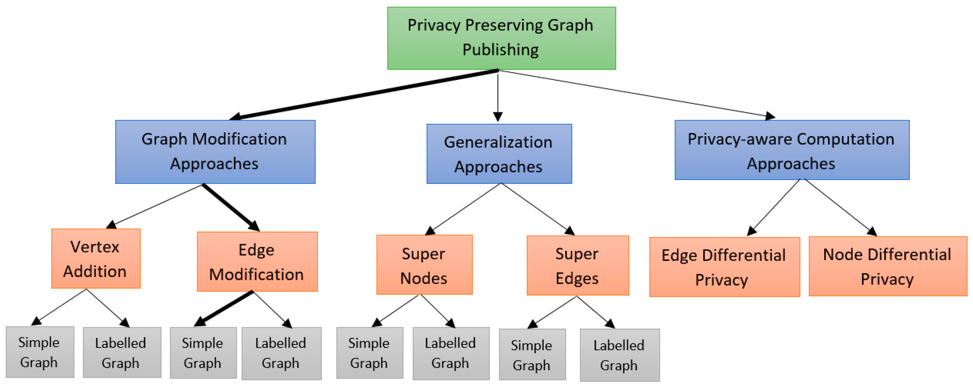
2. Related Work
Graph Modification Techniques
3. Problem Statement
- For all social network graphs, the input k value is determined independently and regardless of the graph structure to be anonymized. This may impose a higher level of privacy than the graph requires, thereby reducing the graph’s utility too much. Additionally, the amount of privacy level applied to the graph may not be sufficient and lead to the disclosure of sensitive information of users. For this reason, it is necessary to determine the privacy level of the graph according to the characteristics of that graph and automatically by the algorithm itself, and in this way, a balance between the level of privacy and the utility of the graph is satisfied.
- The value of the k parameter, the anonymization and privacy level, should be specified as the algorithm input, which is often difficult to find the appropriate k value of the graph for the data owner. As explained before, improper selection of k can reduce privacy or increase information loss and reduce graph utility.
- It should determine the optimal value of the k parameter by the algorithm itself. This way, the data owner’s concerns about the appropriate level of graph privacy are decreased.
- In determining the k value, it should consider the features of the graph degree sequence. As discussed before, considering the graph structure in determining the privacy level of the graph can increase the anonymization of sensitive information and decrease information loss. Therefore, the utility of the anonymized graph increases.
4. FSopt_k Algorithm
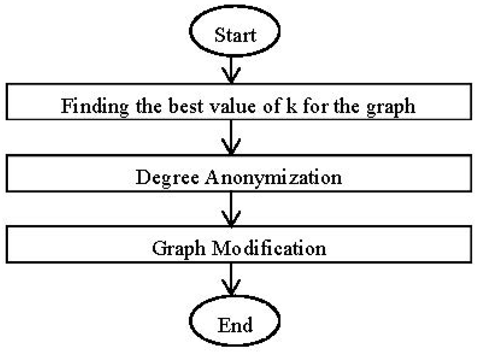
4.1. General Structure of Proposed Method
4.2. Details of the Proposed Algorithm
4.2.1. Finding the Optimal Value of k for the Graph
| Algorithm 1 Finding the optimal value of k |
| Input: graph G |
| Output: the best value of k |
| Create the aggregate vector of G |
| Employ NaFa to find the best solution |
| Compute the best value of k based on the NaFa solution |
| Return k value |
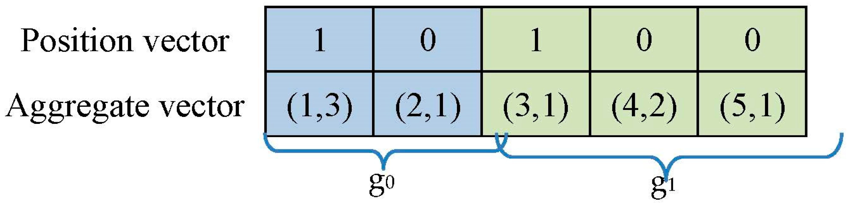
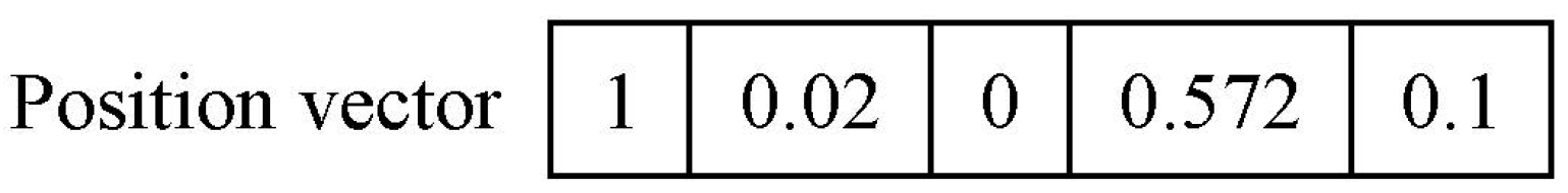
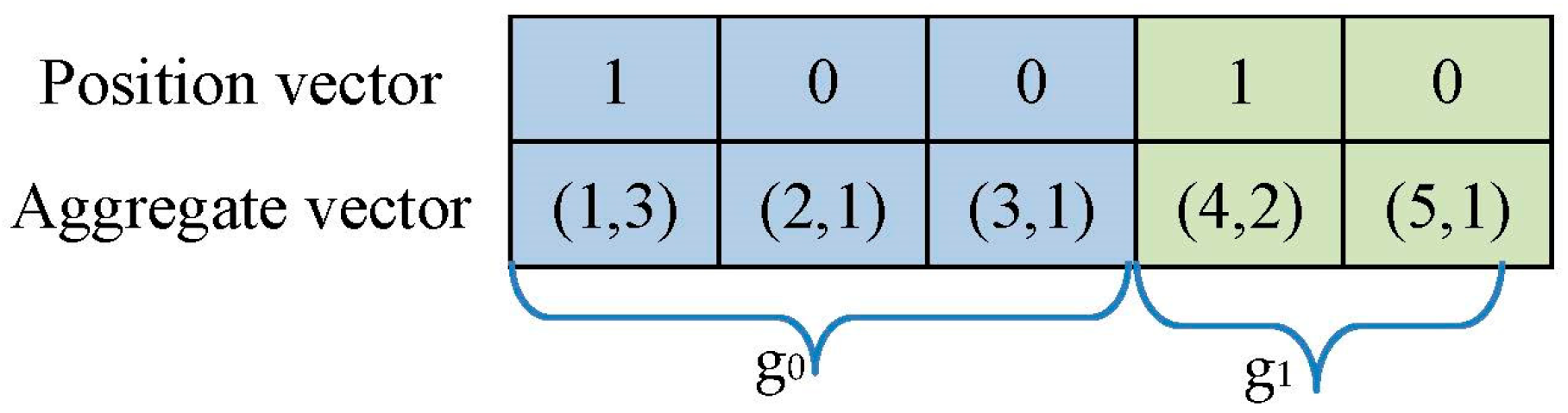
Creating an Aggregate Vector
Employing NaFa to Find the Best Solution
- Initial population creation
- Fitness function
- Creating new population
Compute the Best Value of k Based on the NaFa Solution
4.2.2. Anonymizing the Graph Degree Sequence
4.2.3. Graph Modification
4.3. Time Complexity Analysis
5. Case Study
5.1. Creating an Aggregate Vector
5.2. Employing NaFa to Find the Best Solution
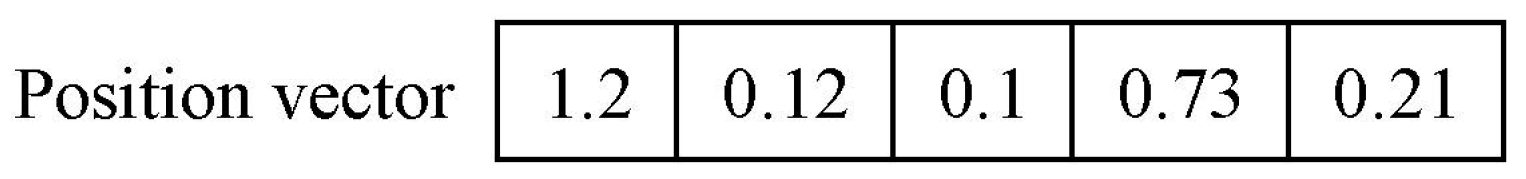
5.2.1. Creating Initial Population
5.2.2. Fitness Function
5.2.3. Creating New Population
6. Experimental Results
6.1. Algorithm Runtime Properties
6.1.1. Datasets
6.1.2. Empirical Results
6.2. Information Loss Metrics
6.2.1. Optimal Value of k
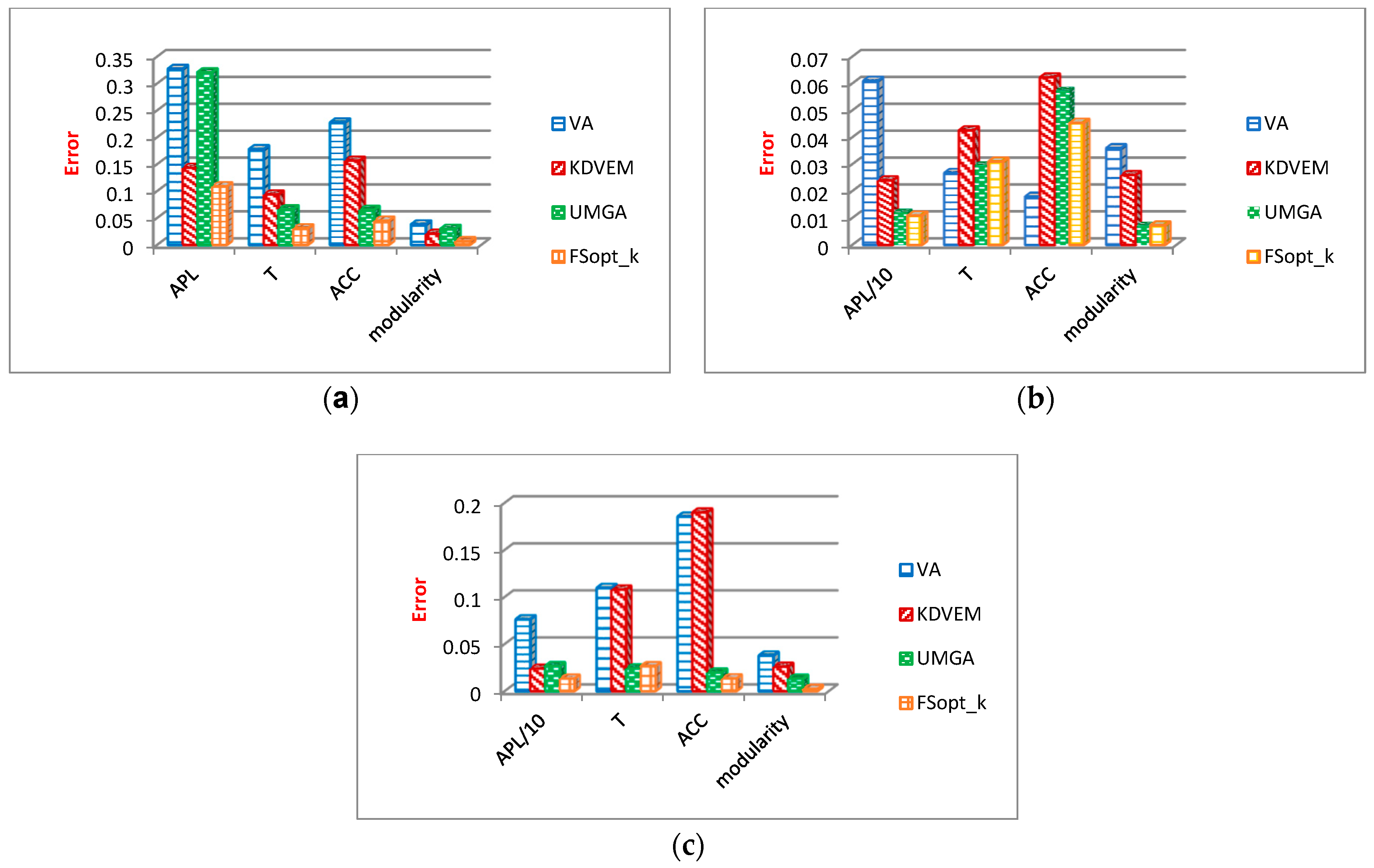
6.2.2. General Properties of Graph Analysis
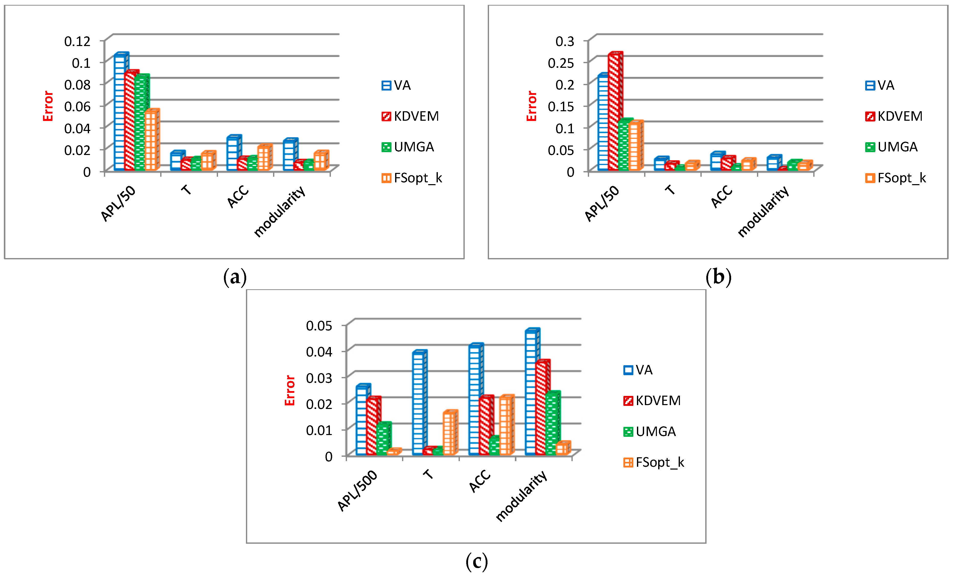
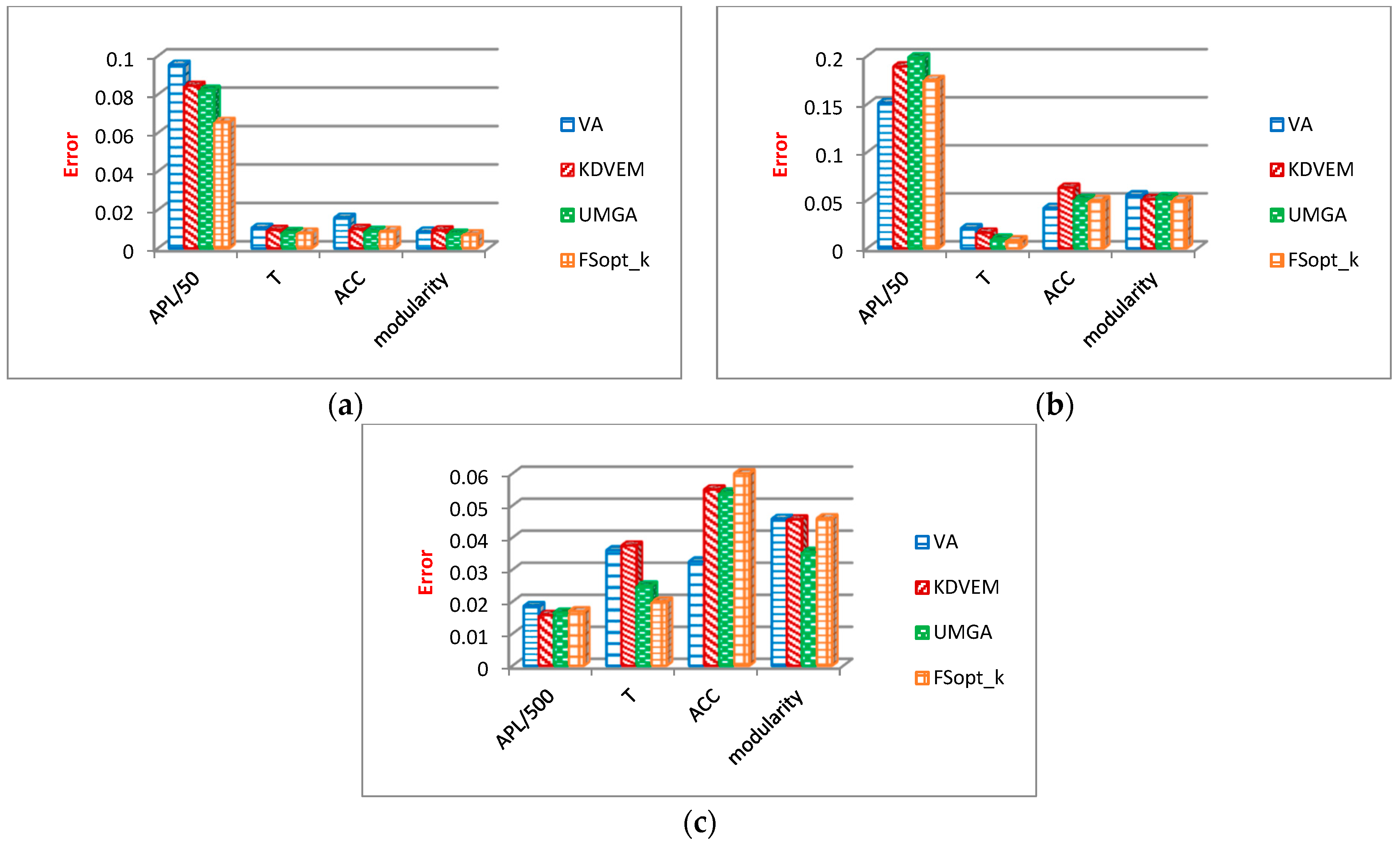
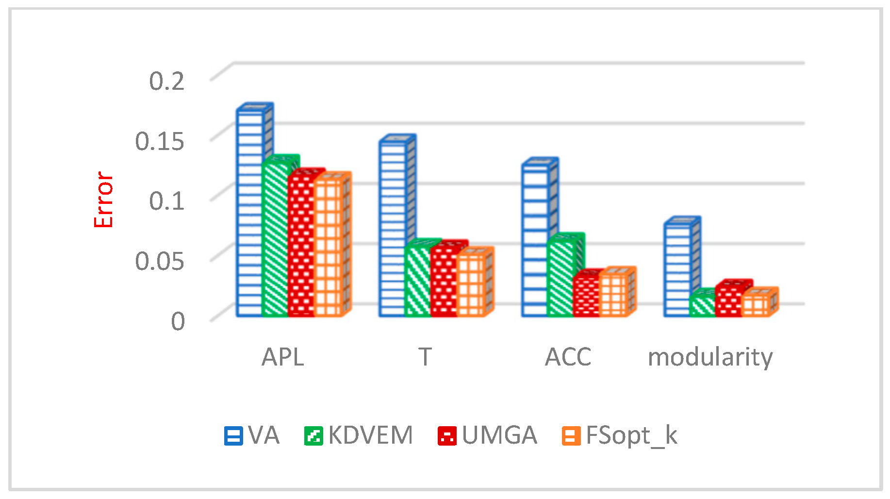
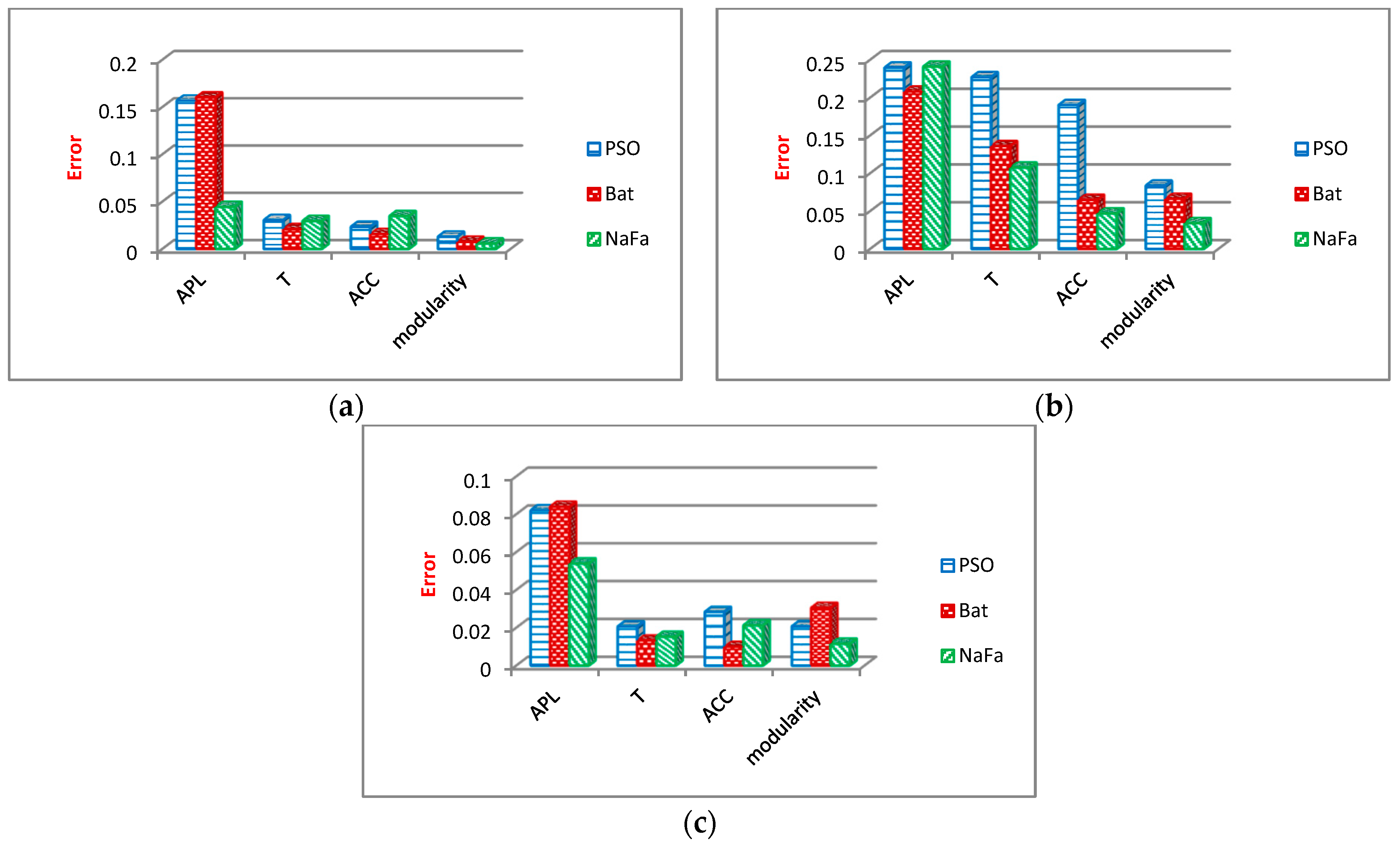
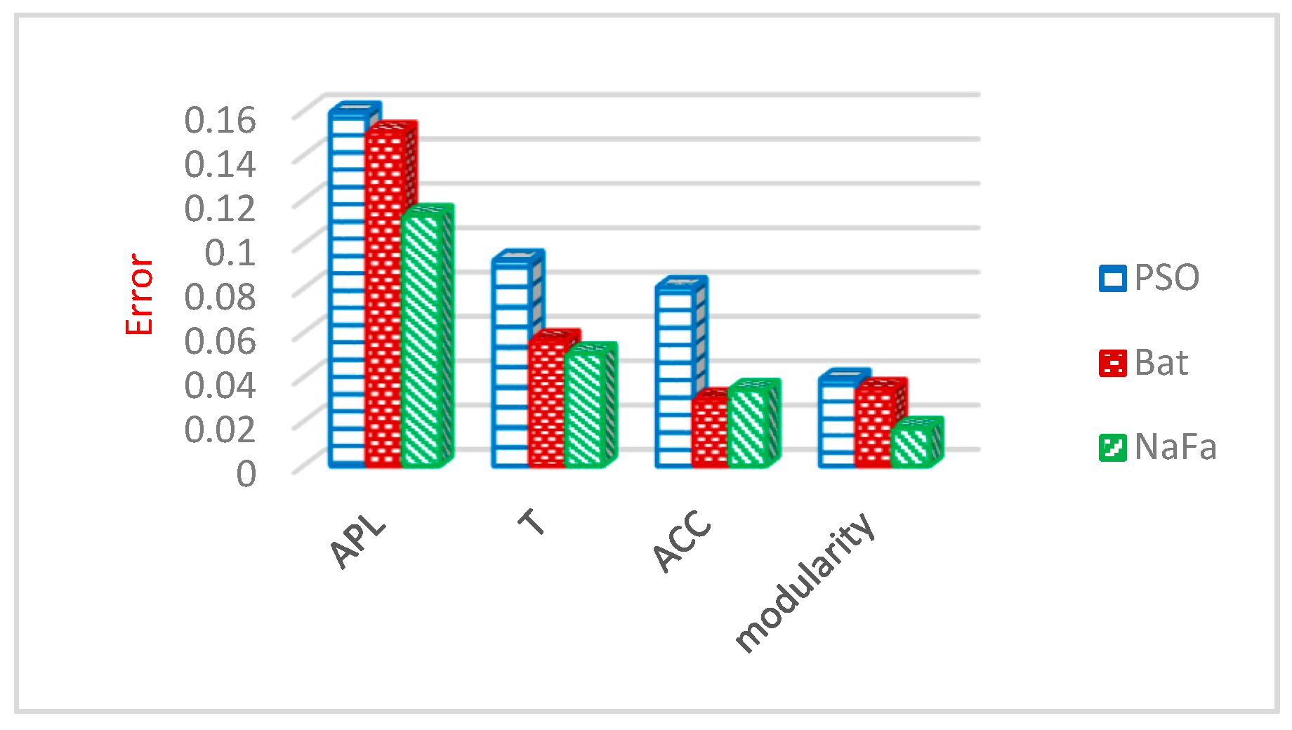
- Average path length (APL) measures the average length of the shortest paths in the social network graph between vertices. This parameter is one of the most important graph analysis criteria and is defined as Equation (25).where d (vi, vj) denotes the shortest path length between each of the vi and vj nodes, and n indicates the number of graph nodes.
- Transitivity (T) is a further criterion utilized to assess FSopt_k, which measures the relative number of triangles in a graph and is defined as Equation (26).where Δ refers to the number of triangles, and ∧ denotes the number of paths with length two.
- Average clustering coefficient (ACC) measures the closeness of the neighbors of each of the graph nodes to the full graph. This criterion is defined in Equation (27).where u shows a node in the graph, n denotes the number of graph nodes, and deg(u) represents the degree of node u.
- Modularity (mod) is one of the criteria used to measure the strength of the network division into modules.
Evaluation Results of General Graph Properties
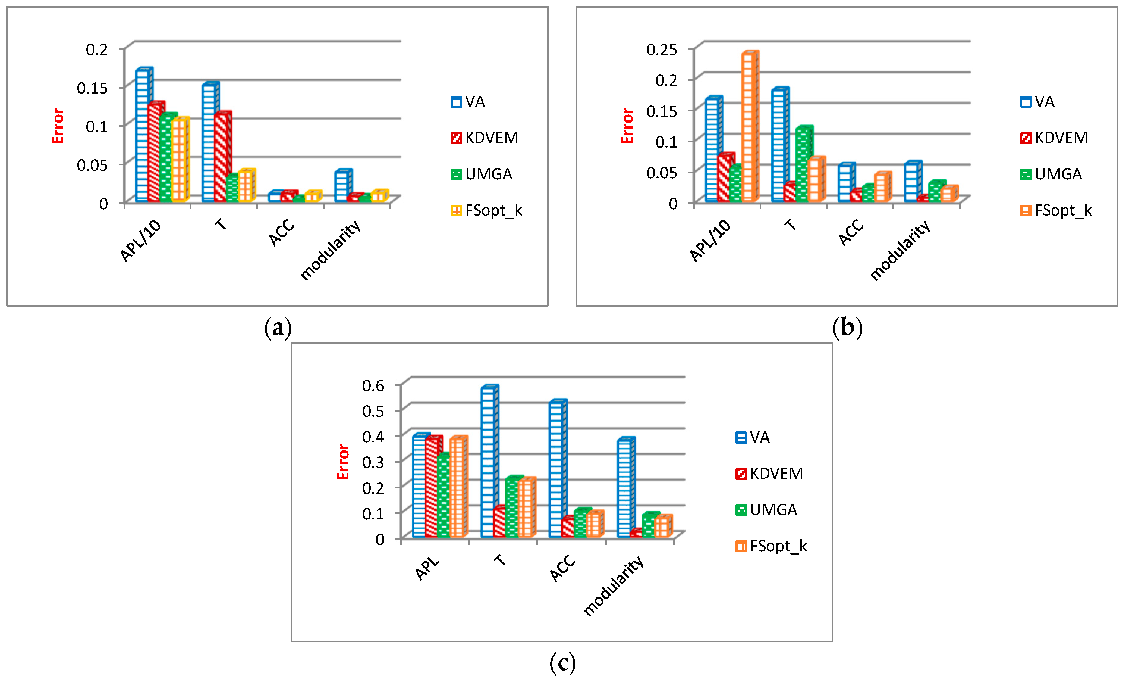
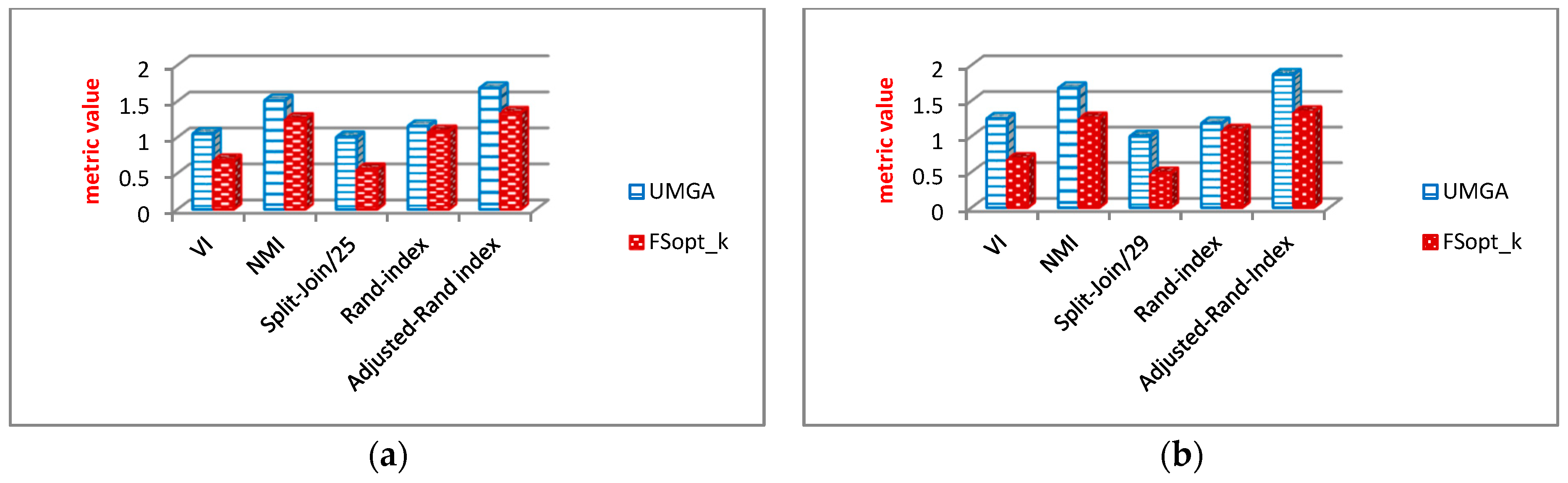
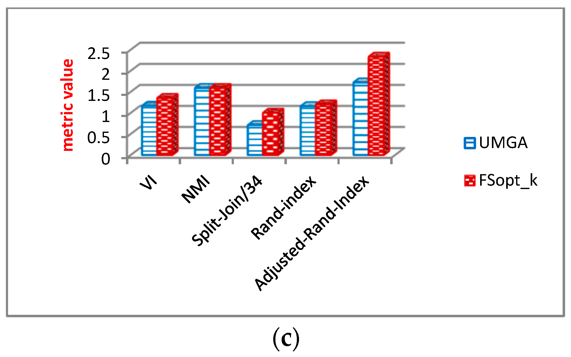
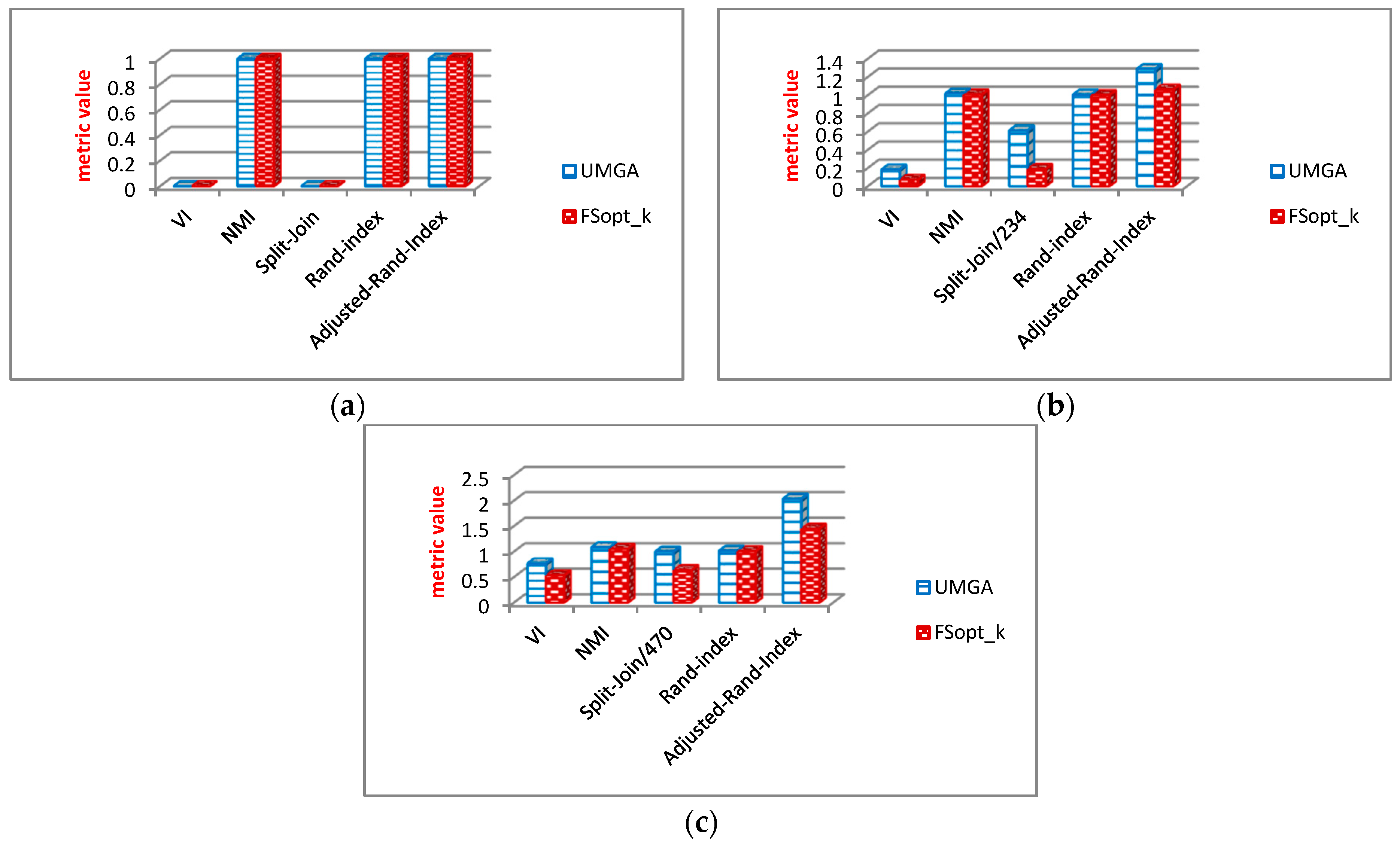
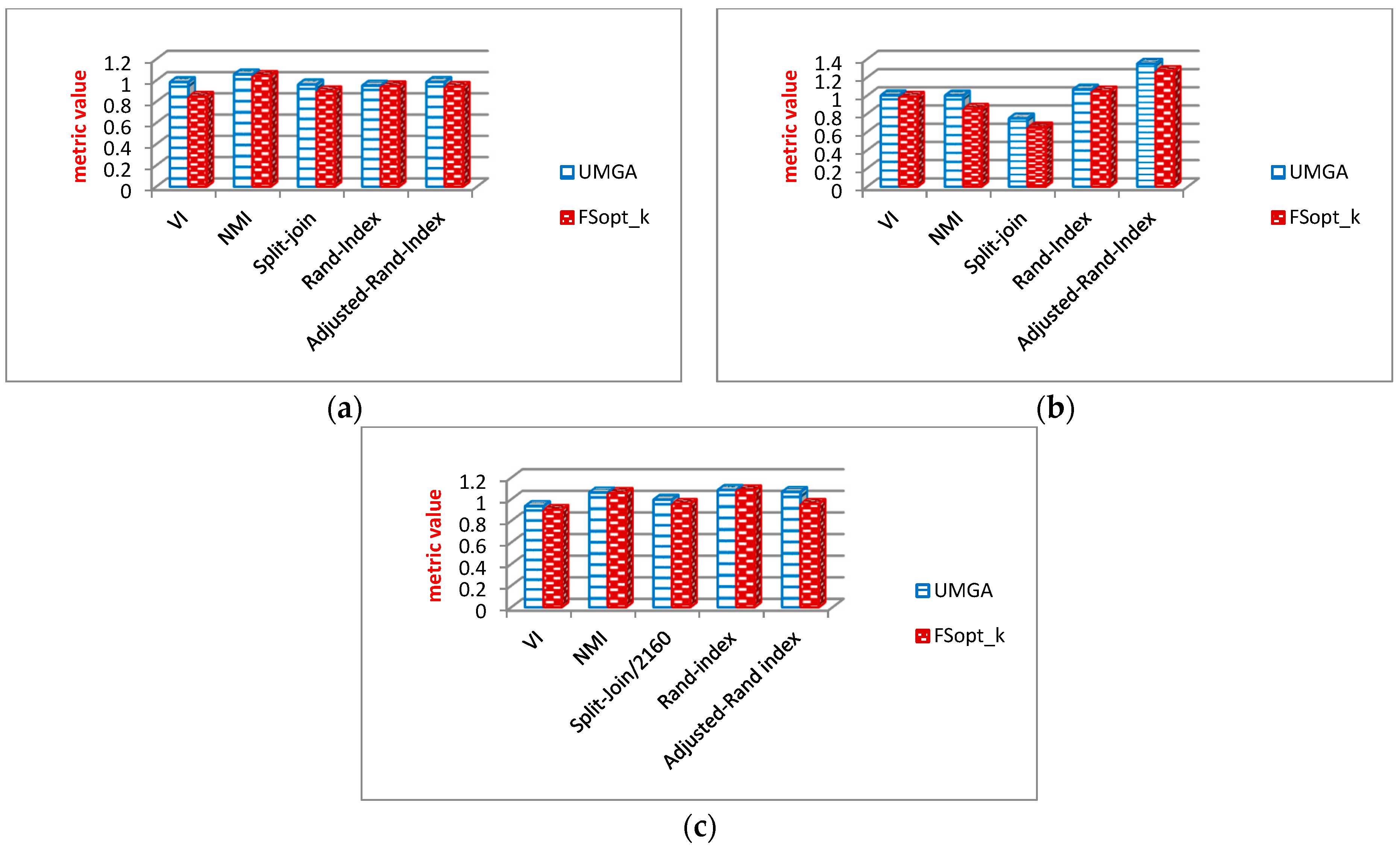
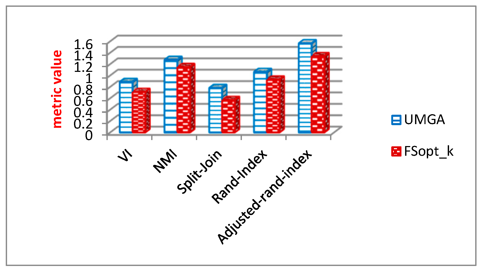
6.2.3. Analysis of Community Structure Metrics
Evaluation Results of Community Structure Metrics
6.3. Comparison of Optimization Algorithms
6.3.1. Evaluation of Runtime of Optimization Algorithms
6.3.2. Evaluation Results of General Graph Properties
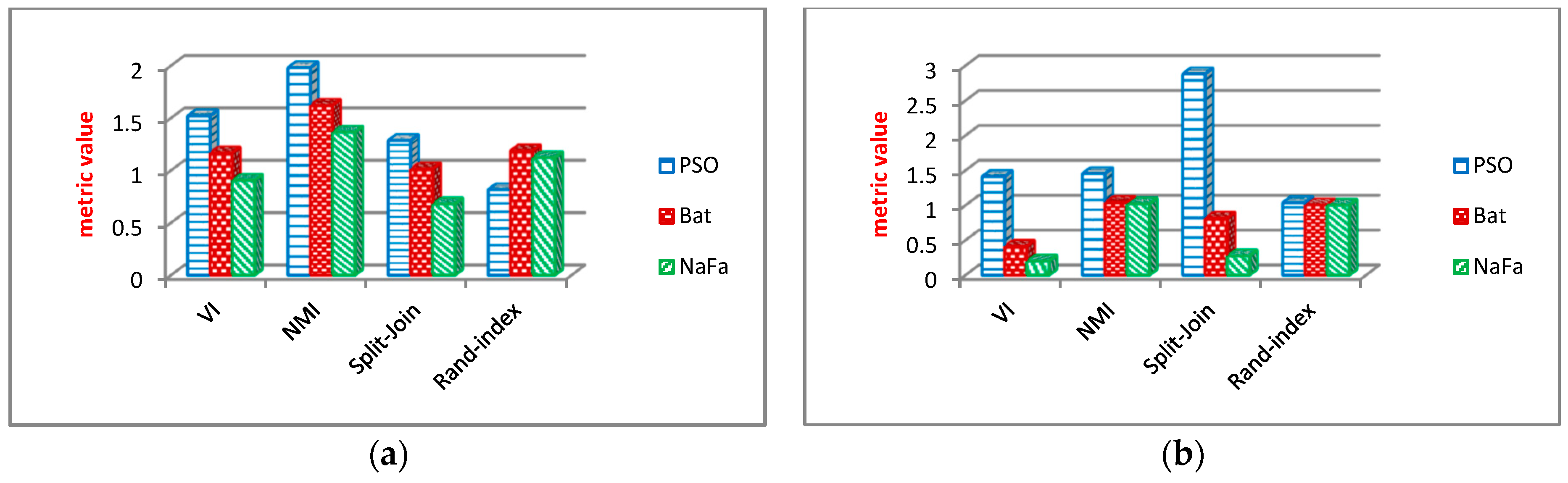
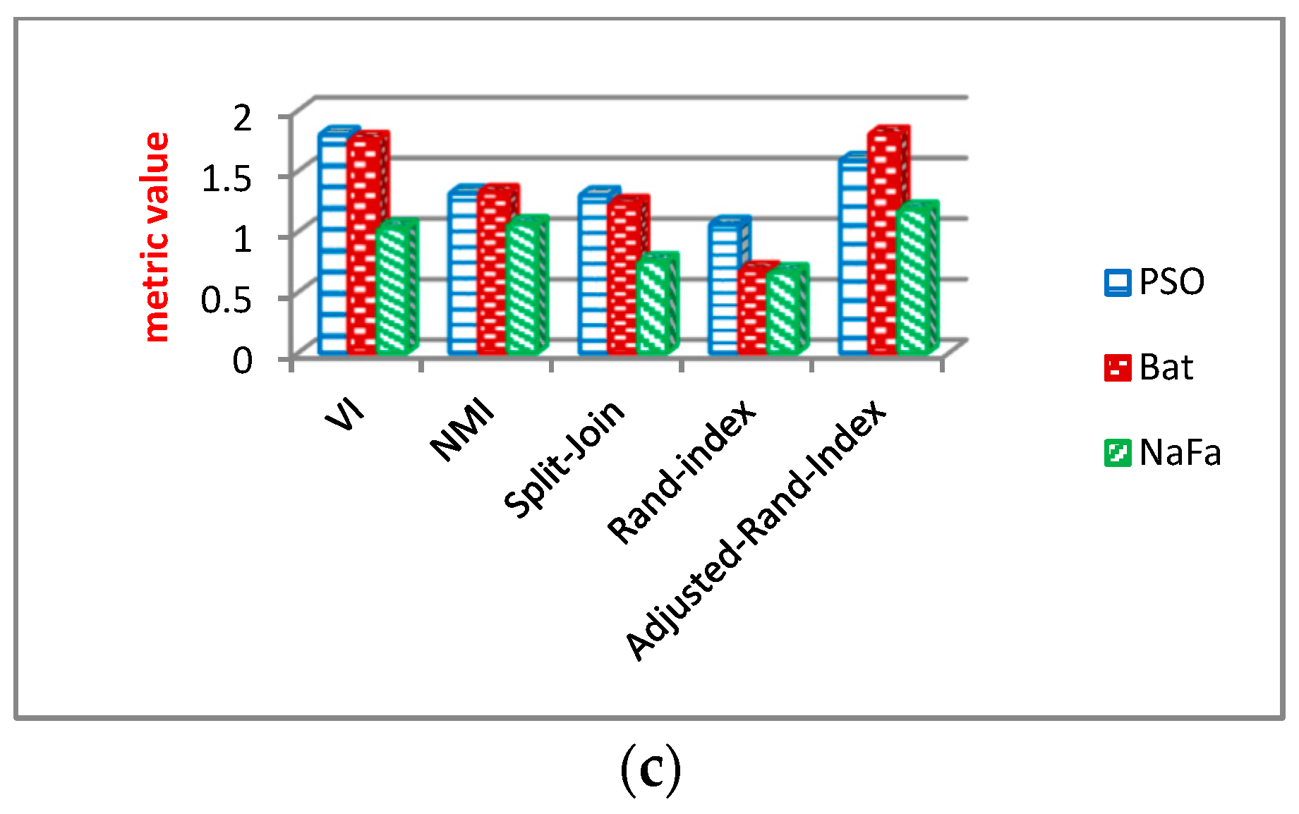
6.3.3. Evaluation Results of Community Structure Metrics
7. Conclusions
Author Contributions
Funding
Informed Consent Statement
Data Availability Statement
Conflicts of Interest
References
- Fung, B.C.M.; Wang, K.; Fu, A.W.-C.; Yu, P.S. Introduction to Privacy-Preserving Data Publishing: Concepts and Techniques, 1st ed.; Chapman and Hall/CRC: Boca Raton, FL, USA, 2011. [Google Scholar]
- Ferri, F.; Grifoni, P.; Guzzo, T. New forms of social and professional digital relationships: The case of Facebook. Soc. Netw. Anal. Min. 2012, 2, 121–137. [Google Scholar] [CrossRef]
- Martin, A.J. Yahoo Dumps 13.5 TB of Users News Interaction Data for Machine Eating. 2016. Available online: https://www.theregister.com/2016/01/14/yahoo_dumps_135tb_of_users_news_interaction_data_for_machine_eating/ (accessed on 1 January 2020).
- Backstrom, L.; Dwork, C.; Kleinberg, J. Wherefore art thou r3579x? In Proceedings of the 16th International Conference on World Wide Web-WWW’07, Banff, AB, Canada, 8–12 May 2007; Volume 54, p. 181. [Google Scholar] [CrossRef]
- Wang, H.; Wang, W.; Zhou, X.; Sun, H.; Zhao, J.; Yu, X. Firefly algorithm with neighborhood attraction. Inf. Sci. 2017, 382–383, 374–387. [Google Scholar] [CrossRef]
- Roma, J.C. Privacy-Preserving and Data Utility in Graph Mining; Universitat Autònoma de Barcelona, Departament d’Enginyeria de la Informació i de les Comunicacions: Barcelona, Spain, 2014. [Google Scholar]
- Dwork, C. Differential Privacy. In International Colloquium on Automata, Languages, and Programming; Springer: Berlin/Heidelberg, Germany, 2006. [Google Scholar]
- Samarati, P. Protecting respondents’ identities in micro-data release. IEEE Trans. Knowl. Data Eng. 2001, 13, 1010–1027. [Google Scholar] [CrossRef] [Green Version]
- Sweeney, L. K-anonymity: A Model for Protecting Privacy. Int. J. Uncertain. Fuzziness Knowl.-Based Syst. 2002, 10, 557–570. [Google Scholar] [CrossRef] [Green Version]
- Liu, K.; Terzi, E. Towards identity anonymization on graphs. In Proceedings of the 2008 ACM SIGMOD International Conference on Management of Data, Vancouver, BC, Canada, 9–12 June 2008; pp. 93–106. [Google Scholar] [CrossRef] [Green Version]
- Zhou, B.; Pei, J. Preserving Privacy in Social Networks Against Neighborhood Attacks. In Proceedings of the 2008 IEEE 24th International Conference on Data Engineering, Cancun, Mexico, 7–12 April 2008; pp. 506–515. [Google Scholar] [CrossRef] [Green Version]
- He, X.; Vaidya, J.; Shafiq, B.; Adam, N.; Atluri, V. Preserving privacy in social networks: A structure-aware approach. In Proceedings of the 2009 IEEE/WIC/ACM International Conference on Web Intelligence, Milan, Italy, 15–18 September 2009; Volume 1, pp. 647–654. [Google Scholar] [CrossRef]
- Tripathy, B.K.; Panda, G.K. A new approach to manage security against neigborhood attacks in social networks. In Proceedings of the 2010 International Conference on Advances in Social Network Analysis and Mining, Odense, Denmark, 9–11 August 2010; pp. 264–269. [Google Scholar] [CrossRef]
- Hay, M.; Miklau, G.; Jensen, D.; Towsley, D.; Weis, P. Resisting Structural Re-identification in Anonymized Social Networks. Proc. VLDB Endow. 2008, 1, 102–114. [Google Scholar] [CrossRef] [Green Version]
- Zou, L.; Chen, L.; Özsu, M.T. K-Automorphism: A General Framework for Privacy Preserving Network Publication. Proc. VLDB Endow. 2009, 2, 946–957. [Google Scholar] [CrossRef] [Green Version]
- Tai, C.; Yu, P.S.S.; Yang, D.-N.; Chen, M.; Yang, D.-N.; Chen, M. Privacy-preserving social network publication against friendship attacks. In Proceedings of the 17th ACM SIGKDD International Conference on Knowledge Discovery and Data Mining-KDD ’11, San Diego, CA, USA, 21–24 August 2011; p. 1262. [Google Scholar] [CrossRef]
- Assam, R.; Brysch, M.; Seidl, T. (k, d)-Core Anonymity: Structural Anonymization of Massive Networks. In Proceedings of the 26th International Conference on Scientific and Statistical Database Management, New York, NY, USA, 30 June–2 July 2014; Volume 17, pp. 1–17. [Google Scholar]
- Feder, T.; Nabar, S.U.; Terzi, E. Anonymizing Graphs. CoRR, abs/0810.5, 1–15, 2008. Available online: http://arxiv.org/abs/0810.5578v1 (accessed on 30 October 2008).
- Stokes, K.; Torra, V. Reidentification and k-anonymity: A model for disclosure risk in graphs. Soft Comput. 2012, 16, 1657–1670. [Google Scholar] [CrossRef] [Green Version]
- Chester, S.; Gaertner, J.; Stege, U.; Venkatesh, S. Anonymizing subsets of social networks with degree constrained subgraphs. In Proceedings of the 2012 IEEE/ACM International Conference on Advances in Social Networks Analysis and Mining, Istanbul, Turkey, 26–29 August 2012; pp. 418–422. [Google Scholar] [CrossRef]
- Das s, E.A.A.; Egecioglu, Ö.; Das, S.; Egecioglu, O.; El Abbadi, A. Anonymizing weighted social network graphs. In Proceedings of the Data Engineering (ICDE), 2010 IEEE 26th International Conference on 2010, Long Beach, CA, USA, 1–6 March 2010; pp. 904–907. [Google Scholar] [CrossRef] [Green Version]
- Kapron, B.; Srivastava, G.; Venkatesh, S. Social network anonymization via edge addition. In Proceedings of the 2011 International Conference on Advances in Social Networks Analysis and Mining, Kaohsiung, Taiwan, 25–27 July 2011; pp. 155–162. [Google Scholar] [CrossRef]
- Zhou, B.; Pei, J. The k-anonymity and l-diversity approaches for privacy preservation in social networks against neighborhood attacks. Knowl. Inf. Syst. 2011, 28, 47–77. [Google Scholar] [CrossRef]
- Chester, S.; Kapron, B.M.; Venkatesh, G.S.S. Complexity of Social Network Anonymization. Soc. Netw. Anal. Min. 2013, 3, 151–166. [Google Scholar] [CrossRef]
- Li, N. T-Closeness: Privacy Beyond k-Anonymity and-Diversity. In Proceedings of the IEEE International Conference on Data Engineering (ICDE), IEEE Computer Society Turkey, Istanbul, Turkey, 15–20 April 2007; pp. 106–115. [Google Scholar]
- Chester, S.; Srivastava, G. Social network privacy for attribute disclosure attacks. In Proceedings of the 2011 International Conference on Advances in Social Networks Analysis and Mining, Kaohsiung, Taiwan, 25–27 July 2011; pp. 445–449. [Google Scholar] [CrossRef]
- Yuan, M.; Chen, L.; Yu, P.S.; Yu, T. Protecting sensitive labels in social network data anonymization. IEEE Trans. Knowl. Data Eng. 2013, 25, 633–647. [Google Scholar] [CrossRef]
- Boldi, P.; Bonchi, F.; Gionis, A.; Tassa, T. Injecting Uncertainty in Graphs for Identity Obfuscation. Proc. VLDB Endow. 2012, 5, 1376–1387. [Google Scholar] [CrossRef] [Green Version]
- Nguyen, H.H.H.; Imine, A.; Est, L.I.N.; Rusinowitch, M. Anonymizing Social Graphs via Uncertainty Semantics. In Proceedings of the 10th ACM Symposium on Information, Computer and Communications Security (ASIA CCS ’15), New York, NY, USA, 14–17 April 2015; pp. 495–506. [Google Scholar] [CrossRef] [Green Version]
- Nguyen, H.H.; Imine, A.; Rusinowitch, M. A maximum variance approach for graph anonymization. In Foundations and Practice of Security. FPS 2014; Lecture Notes in Computer Science Series; Springer: Cham, Switzerland, 2014; Volume 8930, pp. 49–64. [Google Scholar] [CrossRef] [Green Version]
- Park, J.H.; Sung, Y.; Sharma, P.K.; Jeong, Y.-S.; Yi, G. Novel assessment method for accessing private data in social network security services. J. Supercomput. 2017, 73, 3307–3325. [Google Scholar] [CrossRef]
- Rousseau, F.; Casas-Roma, J.; Vazirgiannis, M. Community-preserving anonymization of graphs. Knowl. Inf. Syst. 2018, 54, 315–343. [Google Scholar] [CrossRef]
- Siddula, M.; Li, L.; Li, Y. An Empirical Study on the Privacy Preservation of Online Social Networks. IEEE Access 2018, 6, 19912–19922. [Google Scholar] [CrossRef]
- Li, X.; Yang, Y.; Chen, Y.; Niu, X. A privacy measurement framework for multiple online social networks against social identity linkage. Appl. Sci. 2018, 8, 1790. [Google Scholar] [CrossRef] [Green Version]
- Zhang, X.; Liu, J.; Li, J.; Liu, L. Large-scale Dynamic Social Network Directed Graph K-In&Out-Degree Anonymity Algorithm for Protecting Community Structure. IEEE Access 2019, 99, 108371–108383. [Google Scholar] [CrossRef]
- Siddula, M.; Li, Y.; Cheng, X.; Tian, Z.; Cai, Z. Anonymization in online social networks based on enhanced equi-cardinal clustering. IEEE Trans. Comput. Soc. Syst. 2019, 6, 809–820. [Google Scholar] [CrossRef]
- Kiabod, M.; Dehkordi, M.N.; Barekatain, B. TSRAM: A time-saving k-degree anonymization method in social network. Expert Syst. Appl. 2019, 125, 378–396. [Google Scholar] [CrossRef]
- Bazgana, C.; Cazalsa, P.; Chlebíková, J. Degree-anonymization using edge rotations. Theor. Comput. Sci. 2021, 873, 1–15. [Google Scholar] [CrossRef]
- Al-asbahi, R. Structural Anonymity For Privacy Protection In Social Network. Int. J. Sci. Res. Publ. 2021, 11, 102–107. [Google Scholar] [CrossRef]
- Singh, A.; Singh, M.; Bansal, D.; Sofat, S. Optimised K-anonymisation technique to deal with mutual friends and degree attacks. Int. J. Inf. Comput. Secur. 2021, 14, 281–299. [Google Scholar] [CrossRef]
- Kiabod, M.; Naderi, M.; Barekatain, B. A fast graph modification method for social network anonymization. Expert Syst. Appl. 2021, 180, 115148. [Google Scholar] [CrossRef]
- Ma, N.X.X. TKDA: An Improved Method for K-degree Anonymity in Social Graphs. In Proceedings of the IEEE Symposium on Computers and Communications (ISCC), Rhodes, Greece, 30 June–3 July 2022. [Google Scholar] [CrossRef]
- Ren, X.; Jiang, D. A Personalized (α,β,l,k)-Anonymity Model of Social Network for Protecting Privacy. Wirel. Commun. Mob. Comput. 2022, 2022, 7187528. [Google Scholar] [CrossRef]
- Casas-Roma, J.; Herrera-Joancomartí, J.; Torra, V. k-Degree anonymity and edge selection: Improving data utility in large networks. Knowl. Inf. Syst. 2017, 50, 447–474. [Google Scholar] [CrossRef]
- Csárdi, G.; Nepusz, T. The igraph software package for complex network research. InterJ. Complex Syst. 2006, 1695, 1–9. [Google Scholar] [CrossRef]
- Leskovec, J.; Lang, K.J.; Mahoney, M.W. Community Structure in Large Networks: Natural Cluster Sizes and the Absence of Large Well-Defined Clusters. Internet Math. 2009, 6, 29–123. [Google Scholar] [CrossRef] [Green Version]
- Yang, J.; Leskovec, J. Defining and Evaluating Network Communities based on Ground-truth. In Proceedings of the 2012 IEEE 12th International Conference on Data Mining, Brussels, Belgium, 10–13 December 2012; pp. 745–754. [Google Scholar]
- Chester, S.; Kapron, B.M.; Ramesh, G.; Srivastava, G.; Thomo, A.; Venkatesh, S. Why Waldo befriended the dummy? k-Anonymization of social networks with pseudo-nodes. Soc. Netw. Anal. Min. 2013, 3, 381–399. [Google Scholar] [CrossRef]
- Ma, T.; Zhang, Y.; Cao, J.; Shen, J.; Tang, M.; Tian, Y.; Al-Dhelaan, A.; Al-Rodhaan, M. KDVEM: A k-degree anonymity with vertex and edge modification algorithm. Computing 2015, 97, 1165–1184. [Google Scholar] [CrossRef]
- Lusseau, D.; Schneider, K.; Boisseau, O.J.; Haase, P.; Slooten, E.; Dawson, S.M. The bottlenose dolphin community of doubtful sound features a large proportion of long-lasting associations: Can geographic isolation explain this unique trait? Behav. Ecol. Sociobiol. 2003, 54, 396–405. [Google Scholar] [CrossRef]
- Newman, M.E.J. Finding community structure in networks using the eigenvectors of matrices. Phys. Rev. E 2006, 74, 036104. [Google Scholar] [CrossRef] [Green Version]
- Watts, D.J.; Strogatz, S.H. Collective dynamics of ‘small-world’ networks. Nature 1998, 393, 440–442. [Google Scholar] [CrossRef] [PubMed]
- Danon, L.; Díaz-Guilera, A.; Duch, J.; Arenas, A.; Albert, D.; Duch, J. Comparing community structure identification. J. Stat. Mech. Theory Exp. 2005, 09008, 219–228. [Google Scholar] [CrossRef] [Green Version]
- van Dongen, S. Performance Criteria for Graph Clustering and Markov Cluster Experiments; Technical Report INS-R0012; National Research Institute for Mathematics and Computer Science: Amsterdam, The Netherlands, 2000. [Google Scholar]
- Rand, W.M. Objective Criteria for the Evaluation of Clustering Methods. J. Am. Stat. Assoc. 1971, 66, 846–850. [Google Scholar] [CrossRef]
- Hubert, L.; Arabie, P. Comparing partitions. J. Classif. 1985, 2, 193–218. [Google Scholar] [CrossRef]
- Kennedy, J.; Eberhart, R. Particle Swarm Optimization. In Proceedings of the IEEE International Conference on Neural Networks, Perth, WA, Australia, 27 November–1 December 1995; pp. 1942–1948. [Google Scholar]
- Yang, X. Bat Algorithm: A Novel Approach for Global Engineering Optimization. Eng. Comput. 2012, 29, 464–483. [Google Scholar] [CrossRef] [Green Version]


| References | Graph Type | Method | Characteristics |
|---|---|---|---|
| [44] | Simple, undirected | k-degree sequence anonymity | Edge Modification |
| [32] | Simple, undirected | k-core anonymization | Edge Modification |
| [36] | Labelled, directed | k-anonymity and l-diversity | Vertex and Edge Modification |
| [35] | Dynamic, directed | k-in&out-degree anonymity | Vertex and Edge Modification |
| [37] | Simple, undirected | k-degree sequence anonymity | Edge Modification |
| [39] | Simple, undirected | k-anonymity and l-diversity | Edge Modification |
| [40] | Simple, undirected | k-anonymity | Edge Modification |
| [41] | Simple, undirected | k-degree sequence anonymity | Edge Modification |
| Characteristics | Nodes | Edges | |
|---|---|---|---|
| Data Sets | |||
| Email-Enron | 36,692 | 183,831 | |
| DBLP | 317,080 | 1,049,866 | |
| Youtube | 1,134,890 | 2,987,624 | |
| Algorithm Data Set | FSopt_k (Hours:Minutes:Seconds) | UMGA (Hours:Minutes:Seconds) | |
|---|---|---|---|
| Email-Enron | 0.05 | 00:00:09 | 00:15:36 |
| 0.1 | 00:00:15 | 00:25:24 | |
| 0.2 | 00:00:20 | 00:46:51 | |
| DBLP | 0.05 | 00:08:25 | 1:08:25 |
| 0.1 | 00:09:42 | 1:35:28 | |
| 0.2 | 00:09:52 | 1:58:41 | |
| Youtube | 0.05 | 1:13:32 | 2:39:12 |
| 0.1 | 1:15:40 | 3:55:19 | |
| 0.2 | 1:16:21 | 5:03:06 | |
| Mean | 00:09:29 | 1:32:26 |
| Data Sets | Characteristics | |
|---|---|---|
| Nodes | Edges | |
| Dolphins | 62 | 159 |
| Netscience | 1589 | 2742 |
| Polbooks | 105 | 441 |
| Power Grid | 4941 | 6594 |
| Algorithms | FSopt_k | UMGA | |||||
|---|---|---|---|---|---|---|---|
| Data Set | |||||||
| Desired Utility | Obtained k Value | Obtained Utility | k Value | Utility | |||
| Dolphins | 0.05 | 0.974633443 | 10 | 0.94134 | 8 | 0.973607 | |
| 0.1 | 0.94369499 | 14 | 0.935483 | 13 | 0.938416 | ||
| 0.2 | 0.91612901 | 20 | 0.9149560 | 20 | 0.914956 | ||
| netscience | 0.05 | 0.997917 | 10 | 0.9971 | 13 | 0.9979023 | |
| 0.1 | 0.992014 | 101 | 0.99005 | 106 | 0.9913992 | ||
| 0.2 | 0.98426684 | 219 | 0.9802 | 227 | 0.9844766 | ||
| Power Grid | 0.05 | 0.998594999 | 79 | 0.993636 | 65 | 0.9984933 | |
| 0.1 | 0.99334365 | 248 | 0.992 | 224 | 0.992938 | ||
| 0.2 | 0.9869257 | 520 | 0.9846 | 516 | 0.9861476 | ||
| Polbooks | 0.05 | 0.9415431 | 7 | 0.940935 | 6 | 0.95012 | |
| 0.1 | 0.90262082 | 8 | 0.89991 | 7 | 0.84225 | ||
| 0.2 | 0.936106561 | 11 | 0.93355 | 9 | 0.9512 | ||
| Algorithms | UMGA | NaFa | Bat | PSO | |||||||
|---|---|---|---|---|---|---|---|---|---|---|---|
| Data Set | |||||||||||
| Desired Utility | k Value | Utility | Obtained k Value | Obtained Utility | k Value | Utility | k Value | Utility | |||
| Dolphins | 0.05 | 0.9746334 | 8 | 0.973607 | 10 | 0.94134 | 12 | 0.9346 | 11 | 0.9395 | |
| 0.1 | 0.9436949 | 13 | 0.938416 | 14 | 0.935483 | 9 | 0.9422 | 12 | 0.9332 | ||
| 0.2 | 0.9161290 | 20 | 0.914956 | 20 | 0.9149560 | 15 | 0.9227 | 28 | 0.9104 | ||
| netscience | 0.05 | 0.997917 | 13 | 0.9979023 | 10 | 0.9971 | 32 | 0.9862 | 22 | 0.9948 | |
| 0.1 | 0.992014 | 106 | 0.9913992 | 101 | 0.99005 | 146 | 0.981 | 110 | 0.9861 | ||
| 0.2 | 0.9842668 | 227 | 0.9844766 | 219 | 0.9802 | 321 | 0.9772 | 288 | 0.9684 | ||
| Power Grid | 0.05 | 0.9985949 | 65 | 0.9984933 | 79 | 0.993636 | 105 | 0.9892 | 61 | 0.9924 | |
| 0.1 | 0.9933436 | 224 | 0.992938 | 248 | 0.992 | 301 | 0.9912 | 346 | 0.9916 | ||
| 0.2 | 0.9869257 | 516 | 0.9861476 | 520 | 0.9846 | 699 | 0.9821 | 598 | 0.9864 | ||
Disclaimer/Publisher’s Note: The statements, opinions and data contained in all publications are solely those of the individual author(s) and contributor(s) and not of MDPI and/or the editor(s). MDPI and/or the editor(s) disclaim responsibility for any injury to people or property resulting from any ideas, methods, instructions or products referred to in the content. |
© 2023 by the authors. Licensee MDPI, Basel, Switzerland. This article is an open access article distributed under the terms and conditions of the Creative Commons Attribution (CC BY) license (https://creativecommons.org/licenses/by/4.0/).
Share and Cite
Kiabod, M.; Dehkordi, M.N.; Barekatain, B.; Raahemifar, K. FSopt_k: Finding the Optimal Anonymization Level for a Social Network Graph. Appl. Sci. 2023, 13, 3770. https://doi.org/10.3390/app13063770
Kiabod M, Dehkordi MN, Barekatain B, Raahemifar K. FSopt_k: Finding the Optimal Anonymization Level for a Social Network Graph. Applied Sciences. 2023; 13(6):3770. https://doi.org/10.3390/app13063770
Chicago/Turabian StyleKiabod, Maryam, Mohammad Naderi Dehkordi, Behrang Barekatain, and Kaamran Raahemifar. 2023. "FSopt_k: Finding the Optimal Anonymization Level for a Social Network Graph" Applied Sciences 13, no. 6: 3770. https://doi.org/10.3390/app13063770