Article

A Helmholtz Free Energy Equation of State of CO2-CH4-N2 Fluid Mixtures (ZMS EOS) and Its Applications

1
College of Earth Sciences, Chengdu University of Technology, Chengdu 610059, China
2
School of Earth Sciences and Resources, China University of Geosciences, Beijing 100083, China
*
Author to whom correspondence should be addressed.
Appl. Sci. 2023, 13(6), 3659; https://doi.org/10.3390/app13063659
Submission received: 20 January 2023 / Revised: 6 March 2023 / Accepted: 7 March 2023 / Published: 13 March 2023
(This article belongs to the Special Issue New Advances and Illustrations in Applied Geochemistry)

Abstract

:
An equation of state (EOS) of CH4-N2 fluid mixtures in terms of Helmholtz free energy has been developed by using four mixing parameters, which can reproduce the pressure-volume-temperature-composition (PVTx) and vapor-liquid equilibrium (VLE) properties of CH4-N2 fluid mixtures. The average absolute deviation of all the PVTx data available up to 673.15 K and 1380 bar from this EOS is 0.38%. Combining this EOS of CH4-N2 fluid mixtures and the EOS of CH4-CO2 and CO2-N2 fluid mixtures in our previous work, an EOS of CO2-CH4-N2 fluid mixtures has been developed, which is named ZMS EOS. The ZMS EOS can calculate all thermodynamic properties of ternary CO2-CH4-N2 fluid mixtures and the average absolute deviation of the PVTx data from the ZMS EOS is 0.40% for the CO2-CH4-N2 system. The ZMS EOS can be applied to calculate excess enthalpies of CO2-CH4-N2 fluid mixtures, predict the solubility of CO2-CH4-N2 fluid mixtures in brine and water, and quantitatively estimate the impact of the impurities (CH4 and N2) on the CO2 storage capacity in the CO2 capture and storage (CCS) processes. The ZMS EOS can also be applied to calculate the isochores of CO2-CH4-N2 system in the studies of fluid inclusions. All Fortran computer codes and Origin drawing projects in this paper can be obtained freely from the corresponding author.

1. Introduction

The CO2, CH4 and N2 are important natural fluids, and non-aqueous CO2–CH4–N2 mixtures are often reported in the studies of fluid inclusions [1,2,3]. In recent decades, the amount of greenhouse gas CO2 in the atmosphere has gradually increased because of the development of industry. Numerous studies have shown that CO2 capture and storage (CCS) is an effective method to reduce the amount of CO2 in the atmosphere [4,5,6]. However, CO2 in industrial exhaust gases is usually impure, mixing with other components, such as CH4 and N2 [7,8]. The impurities can affect the design of the CCS processes [9,10,11]. Therefore, predicting thermodynamic properties of the CO2-CH4-N2 fluid mixtures, especially the pressure-volume-temperature-composition (PVTx) and vapor-liquid equilibrium (VLE) properties at different temperatures and pressures, is of great significance for the related CCS and fluid inclusion studies [12,13,14,15].
Although experimental thermodynamic data are the most reliable in the corresponding applications, they are costly and time-consuming to obtain. On the other hand, the predictive EOS is a better choice for us. In the past century, the cubic EOSs (e.g., Peng-Robinson (PR) EOS [16], Soave–Redlich–Kwong (SRK) EOS [17]) originated from the van der Waals EOS [18] are highly preferred for the CCS researchers because of their simplicity. Based on the standard PR EOS, some more accurate EOSs have been presented for the CCS mixtures, such as a model that integrates the classical PR EOS with advanced mixing rules, called the “Peng-Robinson + residual part of excess Helmholtz energy model” [19], and the Enhanced-Predictive-PR78 (E-PPR78) EOS [20]. However, the cubic EOSs cannot well reproduce the PVTx properties of fluids under high pressure-temperature conditions, as can be seen in Section 2. Based on Heyen EOS [21], Heyen et al. [22] simulated the phase equilibria of the CH4-CO2 system below 50 °C and 100 bar; Darimont and Heyen [23] predicted the phase equilibria of the CO2-N2 system below 20 °C and 90 bar. Because cubic EOSs cannot well reproduce the PVTx properties, Thiery et al. [24,25] and Thiery and Dubessy [26] modeled the phase equilibria of the CO2-CH4-N2 system including liquid, vapor and solid by the cubic EOSs and the PVTx properties by the Lee–Kesler correlation [27]. However, these models have the disadvantage of using two EOSs that may cause incoherency of various fluid parameters [28].
In recent years, the Statistical Associating Fluid Theory (SAFT) EOS [29] from Wertheim’s thermodynamic perturbation theory (TPT) has become popular for CCS fluid mixtures. Because it is based on statistical mechanics and has an explicit physical meaning, it has more reliable extrapolation and more accurate predictive capability than traditional empirical models. Many successful modifications of the SAFT-based EOSs have been presented, such as the EOS of perturbed-chain SAFT (PC-SAFT) [30,31], variable range SAFT (SAFT-VR) [32], and Lennard-Jones SAFT (LJ-SAFT) [33]. However, the SAFT EOSs cannot well reproduce experimental VLE data in the near-critical region of the CO2-N2 fluid mixture, as can be seen in the previous work [34]. Up to now, the EOS in terms of Helmholtz free energy is also commonly used to calculate the thermodynamic properties of CCS fluid mixtures [35,36,37,38,39], because the EOS in the form of Helmholtz free energy has high precision, wide temperature-pressure range, and can calculate all thermodynamic properties of the fluids by the derivation from the Helmholtz free energy EOS, such as enthalpy, heat capacity, entropy, etc. The derivation from the Helmholtz free energy EOS is not complex, as can be seen later.
In our previous work [34,40], the EOS in terms of dimensionless Helmholtz free energy for the CH4-CO2 and CO2-N2 fluid mixtures have been established by using four mixing parameters, which have been applied to the studies of the CH4-CO2 and CO2-N2 fluid inclusions. In this work, firstly, the EOS in terms of dimensionless Helmholtz free energy of the CH4-N2 fluid mixture has been developed by the same approach. The ZMS EOS is obtained by combining the binary interaction parameters of CH4-CO2, CO2-N2 and CH4-N2 systems. Experimental data available for the binary CH4-N2 and ternary CO2-CH4-N2 fluid mixtures are used to verify the accuracy of the ZMS EOS. Then the ZMS EOS is applied to calculate the excess enthalpies, the solubility of CO2-CH4-N2 gas mixtures in brine and water, the impact of impurities (CH4 and N2) on the CO2 storage capacity, and the isochores of the CO2-CH4-N2 fluid inclusions.

2. The ZMS EOS

The EOS of the CO2-CH4-N2 mixtures is in terms of dimensionless Helmholtz free energy α , which is represented by
α = α 0 + α r
where α 0 and α r are the ideal-gas part and the residual part of dimensionless Helmholtz free energy. α 0 and α r are defined by
α 0 = i = 1 n x i α i 0 + ln x i
α r = i = 1 n x i α i r δ , τ + α E δ , τ , x
where n is the number of components in the mixture, xi is the mole fraction of component i in the mixture, the superscripts ‘‘0”, “r” and “E” denote the ideal-gas part, the residual part, and the excess of dimensionless Helmholtz free energy, respectively. The subscript i denotes the component i. α i r can be calculated by the EOSs of pure CO2, CH4 and N2 fluids [41,42,43], which are in terms of dimensionless Helmholtz free energy and are recommended as the standard EOSs of pure CO2, CH4 and N2 fluids by the National Institute of Standards and Technology (NIST).
δ and τ of Equation (3) are the reduced mixture density ( δ = ρ / ρ c ) and the inverse reduced mixture temperature ( τ = T c / T ), where ρ and T are the density and temperature of the mixture, and ρ c and T c are the pseudo-critical density and temperature of the mixture. ρ c and T c are defined by
ρ c = i = 1 n x i ρ c i + i = 1 n 1 j = i + 1 n x i x j ζ i j 1
T c = i = 1 n x i T c i + i = 1 n 1 j = i + 1 n x i β i j x j ς i j  
where xj is the mole fraction of component j in the mixture, ρ c i and T c i are the critical density and temperature of component i, respectively. The critical temperatures and densities of the three components considered in this study are listed in Table 1. ζ i j , β i j and ς i j are binary parameters associated with components i and j.
α E of Equation (3) takes the general form developed by Lemmon and Jacobsen (LJ-1999 EOS) [35].
α E δ , τ , x = i = 1 n 1 j = i + 1 n x i x j F i j k = 1 10 N k δ d k τ t k
where Fij is a binary parameter associated with components i and j, Nk, dk and tk are the general parameters independent of fluids, which can be obtained from Lemmon and Jacobsen [35]. There are four binary parameters ( ζ i j , β i j , ς i j and Fij) in the above equations. Binary interaction parameters of CH4-CO2 and CO2-N2 have been determined in previous work [34,40]. In this work, the binary interaction parameters of CH4-N2 systems are obtained by the nonlinear regression of selected experimental data. Since experimental PVTx data available are much more than experimental VLE data, only part of new and accurate experimental PVTx data are selected to fit the parameters to make the PVTx and VLE data keep similar weights in the fitting. In this work, the Levenberg–Marquardt algorithm of the nonlinear least squares method is used for fitting, which is an efficient and widely used mathematical optimization technique. The fitting condition is to minimize the weighted sum of squares of the calculation errors of the equation on the selected experimental PVTx and VLE data. Compared to Newton’s method (e.g., The Newton–Raphson method used in REFPROP [44]), it combines the advantages of two numerical minimization algorithms: the gradient descent method and the Gauss–Newton method, and it has good convergence and robustness. Regressed parameters of the CH4-N2 system are listed in Table 2, which also includes the parameters of CH4-CO2 and CO2-N2 systems from previous studies.

2.1. The Binary CH4-N2 Mixture

The calculated deviations of the PVTx and VLE properties from each experimental data set [45,46,47,48,49,50,51,52,53,54,55,56,57,58,59,60,61,62,63,64,65,66] by this EOS for the CH4-N2 fluid mixture are listed in Table 3. Detail calculation method for the PVTx and VLE properties can be found in Mao et al. [40]. The deviations of the PVTx data are the density deviations, and the temperature and pressure of the experimental PVTx data are up to 673.15 K and 1380 bar, respectively. The deviations of VLE property are the deviations of the vapor-liquid phase equilibrium composition, and the experimental VLE composition covers the full range. The average absolute deviation of all PVTx data from this EOS is 0.38% for the CH4-N2 fluid mixture.
Figure 1 shows the deviations between this EOS and the experimental density data of the CH4-N2 mixture [49,52,54,64] at different pressures. It can be seen in Figure 1 that most of the density deviations are within ±1%, with or close to experimental accuracy. The comparisons between experimental density and the calculated densities by this EOS are shown in Figure 2, where the calculated densities from the PR and SRK EOSs [67] are also included. The errors of three EOSs are also plotted in Figure 2. Figure 2 shows the PR and SRK EOSs cannot well reproduce the PVTx properties, especially under high-pressure conditions. In contrast, the calculated densities from this EOS are in good agreement with experiment data [68].
Figure 3 compares the vapor-liquid phase equilibrium curves calculated from this EOS with experimental data [55,57,59,66] at three temperatures of 170 K, 115 K and 110 K. It can be seen from Figure 3 that the calculated vapor-liquid phase equilibrium curves from this EOS are consistent with experimental data, indicating that this EOS can accurately calculate the vapor-liquid phase equilibrium of CH4-N2 mixture.

2.2. The Ternary CO2-CH4-N2 Mixture

Combining binary interaction parameters of the CH4-CO2, CO2-N2 and CH4-N2 systems, the EOS can also predict the thermodynamic properties of the CO2-CH4-N2 mixture. Here, the experimental PVTx and vapor-liquid equilibrium data are used to verify the accuracy of this EOS for the ternary mixture.
The calculated PVTx deviations for the ternary CO2-CH4-N2 mixture from each experimental data set [1,64,69,70,71] are given in Table 4, where the temperature and pressure of the PVTx data are up to 573.15 K and 1000 bar, and the composition almost covers the full range. The average absolute deviation of all PVTx data from this EOS is 0.40% for the CO2-CH4-N2 fluid mixture. Figure 4 shows the comparison between experimental data [71] and calculated densities for the CO2-CH4-N2 mixture at different temperatures. It can be seen from Figure 4 that calculated densities from this EOS are in good agreement with experiment data, indicating that this EOS has a good predictive ability for the CO2-CH4-N2 mixture.
The vapor-liquid phase equilibrium properties of the ternary CO2-CH4-N2 system are shown in Figure 5, where the curves are calculated from this EOS, and the experimental data are from the literature of [72,73,74]. As can be seen from Figure 5, all the experimental data points in the non-critical region agree well with this EOS, but in the near-critical region (Figure 5c), the calculated values deviate largely from experimental data [72,73,74].

3. The Applications of the ZMS EOS

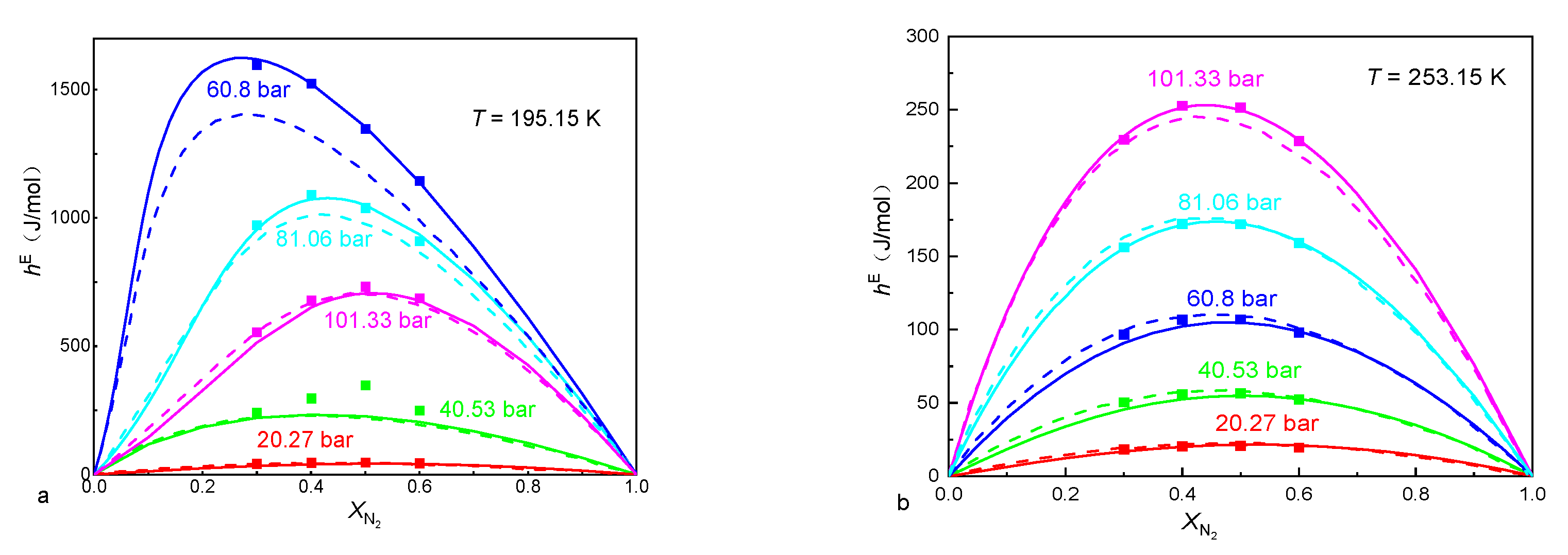
3.1. Calculating Excess Enthalpies

The excess enthalpy ( H E ) is an important thermodynamic property of the mixture for the mixing and separation processes, which is defined by
H E = H m i x i H i P , T
where H m is the enthalpy of the mixture, H i is the enthalpy of pure component i, and xi is the mole fraction of component i in the mixture. According to the thermodynamic relationship between Helmholtz free energy and enthalpy, H m and H i are given by
H m = R T 1 + τ α τ 0 + α τ r + δ α δ r
H i = R T 1 + τ i α τ i 0 + α τ i r + δ i α δ i r
where α τ 0 = α 0 τ δ , α τ r = α r τ δ , α δ r = α r δ τ , α τ i 0 = α i 0 τ i δ i , α τ i r = α i r τ i δ i and α δ i r = α i r δ i τ i . δ i and τ i are the reduced density and inverse reduced temperature of pure component i, which are defined by
δ i = ρ i / ρ c i
τ i = T c i / T
where ρ i is the density of component i. Based on Equations (8)–(11), H m can be calculated by this EOS of the CO2-CH4-N2 fluid mixtures and H i can be calculated by the above-mentioned equations of pure CO2, CH4 and N2 fluids.
The calculated excess enthalpy curves of the CH4-CO2 and CO2-N2 mixtures are, respectively, shown in Figure 6 and Figure 7, where the experimental data [75,76] are included for comparison. The following EOSs are also included for comparison: the standard Peng–Robinson (PR) EOS, either optimized (optimal kij) or not (kij = 0); the PR EOS with the residual part of the Wilson excess Helmholtz energy model (PR + EOS/ a r e s E , W i l s o n ) [19]. It can be seen from Figure 6 and Figure 7 that this EOS is more accurate than the standard PR EOS, either optimized (optimal kij) or not (kij = 0) at most cases. In general, the PR + EOS/ a r e s E , W i l s o n and this EOS shows a similar predictive capability for the excess enthalpies of the CH4-CO2 mixture. However, this EOS is slightly more accurate than the PR + EOS/ a r e s E , W i l s o n for the CO2-N2 mixture at low pressures.
Figure 8 compares the excess enthalpy curves of the CH4-N2 mixture calculated from the ZMS EOS with experimental data [77], and enthalpies calculated from the Enhanced-Predictive-PR78 (E-PPR78) EOS [20] are also added for comparison. Figure 8a shows the ZMSEOS are significantly more accurate than the (E-PPR78) EOS at high and middle pressures. Figure 8b shows the enthalpies of mixing calculated from the E-PPR78 EOS are slightly better than those of the ZMS EOS at low and middle pressures, but the enthalpies of mixing calculated from the ZMS EOS are better than those from the E-PPR78 EOS at P = 101.33 bar.

3.2. Calculating the Solubility of CO2-CH4-N2 Mixtures in Aqueous Electrolyte Solution

The solubility of the CO2-CH4-N2 gas mixtures in the electrolyte solutions can provide the quantitative assessment for the storage of CO2 in deep saline aquifers. According to the thermodynamic principle, when the CO2-CH4-N2 gas mixtures reach dissolution equilibrium in the electrolyte solution, the chemical potential of component i in the liquid phase ( μ i L ) and its chemical potential in the vapor phase ( μ i V ) are equal. The chemical potential can be written in terms of fugacity in the vapor phase and activity in the liquid phase
μ i L = μ i L 0 + R T ln m i γ i
μ i V = μ i V 0 + R T ln φ i y i P
where i is the gas component in vapor mixtures, and P is the pressure in bar. yi is the molar fraction of i in the vapor phase, φ i is the fugacity coefficient of i in the vapor phase and mi is the solubility of i in the liquid phase in mol/kg. γ i is the activity coefficient of component i in the liquid phase. μ i L 0   and μ i V 0 are the standard chemical potential of i in the liquid and vapor phase, respectively.
At the dissolution phase equilibrium, μ i V = μ i L . From Equations (12) and (13), we can obtain
ln m i = ln y i P + ln φ i μ i L 0 μ i V 0 R T ln γ i
Since the water content in the vapor phase at equilibrium is generally small, it has a negligible effect on the fugacity coefficient. When calculating the fugacity coefficient, the water content in the vapor phase can be ignored, the vapor phase can be approximated as the CO2-CH4-N2 system and the mole fraction of gas component i in the vapor phase is expressed as y i . Consequently, φ i can be calculated from the ZMS EOS developed in this work.
Pitzer activity coefficient model [78] is chosen to calculate γ i
ln γ i = c 2 λ i c m c + a 2 λ i a m a + c a ζ i c a m c m a
where λ and ζ are second-order and third-order interaction parameters, respectively; c and a refer to cation and anion, respectively. Substituting Equation (15) into Equation (14) yields
ln m i = ln y i P + ln φ i μ i L 0 μ i V 0 R T c 2 λ i c m c a 2 λ i a m a c a ζ i c a m c m a a
As can be seen from Equation (17), mi is related to the difference between μ i L 0 and μ i V 0 , and is not related to the specific value of μ i L 0 or μ i V 0 . Therefore, to simplify the model, μ i V 0 is assumed to be zero. Equation (16) can be simplified as
ln m i = ln y i P + ln φ i μ i L 0 R T c 2 λ i c m c a 2 λ i a m a c a ζ i c a m c m a
where μ i L 0 R T , λ and ζ are the function of temperature and pressure, and the parameters can be determined by the solubility model of pure gases (CO2, CH4, N2). Since the 1980s, many solubility models for CO2, CH4 and N2 gases in pure water and brine have been developed [79,80,81,82,83,84,85,86,87,88,89,90,91], most of which do not exceed 473 K and 1000 bar. Among them, the solubility models of CH4, CO2 and N2 established by Mao and co-workers [83,86,91] are applicable to a wider range of temperature, pressure, and salinity with higher accuracy. They have been chosen as the solubility models of pure CH4, CO2 and N2 gases in this work. Table 5 lists the applicable temperature, pressure, and salinity ranges of these solubility models for pure gases.
To verify the accuracy of the predictions, the experimental data for the solubility of the CO2-CH4-N2 gas mixtures are compared with the calculated results. Figure 9 compares the experimental data on the solubility of the CH4-CO2 mixture in pure water [92,93] for the temperature range of 324.5–375.5 K and the pressure range of 100–750 bar, and it can be seen that the agreement is very good.
The solubility experimental data of the CO2-N2 gas mixture in pure water [94] and the calculated results are compared in Figure 10, where the temperature range is 308.15–318.15 K and the pressure range is 80–160 bar. As can be seen from Figure 10 the predictive results are in good agreement with the experimental data. The average absolute deviations between the calculated N2 and CO2 solubility of this model and the experimental data are 6.04% and 1.52%, respectively. Figure 11 compares the solubility experimental data of the CO2-N2 gas mixture in saline water. The average absolute deviations between the calculated N2 and CO2 solubility and the experimental data are 2.04% and 2.49%, respectively.

3.3. The Impact of Impurities (CH4 and N2) on the CO2 Storage Capacity

CH4 and N2 are non-condensable impurities, which reduce the CO2 storage capacity in geological formations. Based on the EOS of the CO2-CH4-N2 fluid mixtures, the impact of CH4 and N2 on CO2 storage capacity can be calculated quantitatively by the normalized storage capacity proposed by Wang et al. [9]. For a certain reservoir with a certain volume, the normalized storage capacity of the CO2-CH4-N2 gas mixtures is shown as
A A CO 2 = ρ ρ CO 2 ( 1 + M CH 4 M CO 2 + M N 2 M CO 2 )
where A and A CO 2 are the mass of CO2 in the mixtures and the mass of pure CO2 under the same volume, respectively. ρ CO 2 and ρ are the density of the pure CO2 and CO2-CH4-N2 gas mixtures, respectively; M CH 4 ,   M N 2 and M CO 2 are the mass of CH4, N2, and CO2 in the mixture, respectively. A / A CO 2 is the ratio of the mass of CO2 per unit volume in the mixture to that in the pure state. The value of A / A CO 2 can be viewed as the normalized storage capacity for CO2 (i.e., the storage capacity for structural trapping of CO2). For pure CO2, the normalized storage capacity ( A / A CO 2 ) is 1. For the CO2-CH4-N2 gas mixtures of a given composition, M CH 4 , M N 2   and M CO 2 are also known. ρ CO 2 can be calculated by the above-mentioned equation of pure CO2 fluid and ρ can be calculated by the ZMS EOS.
The normalized storage capacity of the CO2-CH4-N2 fluid mixture calculated by the ZMS EOS is plotted in Figure 12. Figure 12a shows the normalized storage capacity of a given composition at different temperatures. With the increase in pressure, the normalized storage capacity decreases at first and then increases, and there is a minimum point. When the temperature changes, the pressure corresponding to the lowest point of the normalized storage also changes. Figure 12b shows the normalized storage capacity of different compositions at the same temperature, which indicates that the content of impurities is much larger and the normalized storage capacity is much smaller.

3.4. Isochores of the CO2-CH4-N2 fluid Inclusions

In the studies of fluid inclusions, the isochores (pressure-temperature relation at constant density and composition) are frequently used to estimate the trapping temperatures and pressures.
Based on the EOS of the CO2-CH4-N2 fluid mixtures, isochores of the CO2-CH4-N2 inclusions can be calculated by the following equation:
P δ , τ , x = ρ R T 1 + δ α δ r
The calculated isochores of the CO2-CH4-N2 inclusions at two different compositions are plotted in Figure 13, from which it can be seen that the isochores of the CO2-CH4-N2 inclusions are a bit curved.
This section may be divided into subheadings. It should provide a concise and precise description of the experimental results, their interpretation, as well as the experimental conclusions that can be drawn.

4. Conclusions

A fundamental EOS for the Helmholtz free energy of the CH4-N2 mixture has been developed by using four binary interaction parameters. Comparisons with experimental PVTx and VLE data available showed that the EOS can satisfactorily reproduce the experimental volumetric and vapor-liquid phase equilibria data of binary CH4-N2 mixtures up to 673.15 K and 1380 bar, with or close to experimental accuracy. Combining this EOS of the CH4-N2 fluid mixtures and the EOS of the CH4-CO2 and CO2-N2 fluid mixtures developed in our previous work, an EOS of ternary CO2-CH4-N2 fluid mixtures has been presented, which is named ZMS EOS. The ZMS EOS can be applied to calculate excess enthalpies, predict the solubility of the CO2-CH4-N2 gas mixtures in water and brine, estimate the impurities CH4 and N2 on the CO2 storage capacity, and calculate the isochores of the CO2-CH4-N2 fluid mixtures.

Author Contributions

J.Z.: Conceptualization, Software, Investigation, Writing—original. S.M.: Supervision, Methodology, Writing—review, and editing. Z.S.: Investigation, Software, Validation. All authors have read and agreed to the published version of the manuscript.

Funding

This research was funded by the National Natural Science Foundation of China (Grant No. 42073056) and Everest Scientific Research Program of Chengdu University of Technology (80000-2021ZF11419).

Institutional Review Board Statement

Not applicable.

Informed Consent Statement

Not applicable.

Data Availability Statement

Not applicable.

Conflicts of Interest

The authors declare that they have no known competing financial interests or personal relationships that could have appeared to influence the work reported in this paper.

References

  1. Le, V.H.; Caumon, M.C.; Tarantola, A.; Randi, A.; Robert, P.; Mullis, J. Calibration data for simultaneous determination of PVX properties of binary and ternary CO2-CH4-N2 gas mixtures by Raman spectroscopy over 5–600 bar: Application to natural fluid inclusions. Chem. Geol. 2020, 552, 119783. [Google Scholar] [CrossRef]
  2. Caumon, M.C.; Tarantola, A.; Wang, W. Raman spectra of gas mixtures in fluid inclusions: Effect of quartz birefringence on composition measurement. J. Raman Spectrosc. 2020, 51, 1868–1873. [Google Scholar] [CrossRef]
  3. Lüders, V.; Plessen, B.; di Primio, R. Stable carbon isotopic ratios of CH4–CO2-bearing fluid inclusions in fracture-fill mineralization from the Lower Saxony Basin (Germany)–A tool for tracing gas sources and maturity. Mar. Pet. Geol. 2012, 30, 174–183. [Google Scholar] [CrossRef]
  4. Gaurina-Međimurec, N.; Mavar, K.N. Carbon capture and storage (CCS): Geological sequestration of CO2. In CO2 Sequestration; IntechOpen: London, UK, 2019; pp. 1–21. [Google Scholar] [CrossRef] [Green Version]
  5. Pires, J.; Martins, F.; Alvim-Ferraz, M.; Simões, M. Recent developments on carbon capture and storage: An overview. Chem. Eng. Res. Des. 2011, 89, 1446–1460. [Google Scholar] [CrossRef]
  6. Bui, M.; Adjiman, C.S.; Bardow, A.; Anthony, E.J.; Boston, A.; Brown, S.; Fennell, P.S.; Fuss, S.; Galindo, A.; Hackett, L.A. Carbon capture and storage (CCS): The way forward. Energy Environ. Sci. 2018, 11, 1062–1176. [Google Scholar] [CrossRef] [Green Version]
  7. Chapoy, A.; Burgass, R.; Tohidi, B.; Austell, J.M.; Eickhoff, C. Effect of common impurities on the phase behavior of carbon-dioxide-rich systems: Minimizing the risk of hydrate formation and two-phase flow. SPE J. 2011, 16, 921–930. [Google Scholar] [CrossRef]
  8. Thoutam, P.; Rezaei Gomari, S.; Chapoy, A.; Ahmad, F.; Islam, M. Study on CO2 hydrate formation kinetics in saline water in the presence of low concentrations of CH4. ACS Omega 2019, 4, 18210–18218. [Google Scholar] [CrossRef] [Green Version]
  9. Wang, J.; Ryan, D.; Anthony, E.J.; Wildgust, N.; Aiken, T. Effects of impurities on CO2 transport, injection and storage. Energy Procedia 2011, 4, 3071–3078. [Google Scholar] [CrossRef] [Green Version]
  10. Wetenhall, B.; Aghajani, H.; Chalmers, H.; Benson, S.; Ferrari, M.; Li, J.; Race, J.; Singh, P.; Davison, J. Impact of CO2 impurity on CO2 compression, liquefaction and transportation. Energy Procedia 2014, 63, 2764–2778. [Google Scholar] [CrossRef] [Green Version]
  11. Blanco, S.T.; Rivas, C.; Fernández, J.; Artal, M.; Velasco, I. Influence of methane in CO2 transport and storage for CCS technology. Environ. Sci. Technol. 2012, 46, 13016–13023. [Google Scholar] [CrossRef]
  12. Li, H.; Yan, J. Impact of impurities in CO2-fluids on CO2 transport process. In Turbo Expo: Power for Land, Sea, and Air; American Society of Mechanical Engineers: Barcelona, Spain, 2006; pp. 367–375. [Google Scholar]
  13. Li, H.; Yan, J. Impacts of equations of state (EOS) and impurities on the volume calculation of CO2 mixtures in the applications of CO2 capture and storage (CCS) processes. Appl. Energy 2009, 86, 2760–2770. [Google Scholar] [CrossRef]
  14. Tenorio, M.J.; Parrott, A.J.; Calladine, J.A.; Sanchez Vicente, Y.; Cresswell, A.J.; Graham, R.S.; Drage, T.C.; Poliakoff, M.; Ke, J.; George, M.W. Measurement of the vapour–liquid equilibrium of binary and ternary mixtures of CO2, N2 and H2, systems which are of relevance to CCS technology. Int. J. Greenh. Gas Control 2015, 41, 68–81. [Google Scholar] [CrossRef]
  15. Shi, G.U.; Tropper, P.; Cui, W.; Tan, J.; Wang, C. Methane (CH4)-bearing fluid inclusions in the Myanmar jadeitite. Geochem. J. 2005, 39, 503–516. [Google Scholar] [CrossRef] [Green Version]
  16. Peng, D.Y.; Robinson, D.B. A new two-constant equation of state. Ind. Eng. Chem. Fundam. 1976, 15, 59–64. [Google Scholar] [CrossRef]
  17. Soave, G. Equilibrium constants from a modified Redlich-Kwong equation of state. Chem. Eng. Sci. 1972, 27, 1197–1203. [Google Scholar] [CrossRef]
  18. Van der Waals, J. On the Continuity of the Gas and Liquid State; Leiden University: Leiden, The Netherlands, 1873. [Google Scholar]
  19. Lasala, S.; Chiesa, P.; Privat, R.; Jaubert, J.N. Measurement and prediction of multi-property data of CO2-N2-O2-CH4 mixtures with the “Peng-Robinson+ residual Helmholtz energy-based” model. Fluid Phase Equilibria 2017, 437, 166–180. [Google Scholar] [CrossRef]
  20. Xu, X.; Lasala, S.; Privat, R.; Jaubert, J.N. E-PPR78: A proper cubic EOS for modelling fluids involved in the design and operation of carbon dioxide capture and storage (CCS) processes. Int. J. Greenh. Gas Control 2017, 56, 126–154. [Google Scholar] [CrossRef]
  21. Heyen, G. An equation of state with extended range of application. In Proceedings of the Second World Congress of Chemical Engineering, Montreal, QC, Canada, 4–9 October 1981. [Google Scholar]
  22. Heyen, G.; Ramboz, C.; Dubessy, J. Modelling of phase equilibria in the system CO2–CH4 below 50 °C and 100 bar. Appl. Incl. Fluids Fr. Comptes Rendus Acad. Sci. Paris 1982, 294, 203–206. [Google Scholar]
  23. Darimont, A.; Heyen, G. Simulation des équilibres de phases dans le système CO2-N2. Application aux inclusions fluides. Bull. Minéralogie 1988, 111, 179–182. [Google Scholar] [CrossRef]
  24. Thiery, R.; Vidal, J.; Dubessy, J. Phase equilibria modelling applied to fluid inclusions: Liquid-vapour equilibria and calculation of the molar volume in the CO2-CH4N2 system. Geochim. Cosmochim. Acta 1994, 58, 1073–1082. [Google Scholar] [CrossRef]
  25. Thiéry, R.; Van Den Kerkhof, A.M.; Dubessy, J. vX properties of CH4-CO2 and CO2-N2 fluid inclusions: Modelling for T < 31 °C and P < 400 bars. Eur. J. Miner. 1994, 6, 753–771. [Google Scholar]
  26. Thiéry, R.; Dubessy, J. Improved modelling of vapour-liquid equilibria up to the critical region. Application to the CO2-CH4- N2 system. Fluid Phase Equilibria 1996, 121, 111–123. [Google Scholar] [CrossRef]
  27. Lee, B.I.; Kesler, M.G. A generalized thermodynamic correlation based on three-parameter corresponding states. AIChE J. 1975, 21, 510–527. [Google Scholar] [CrossRef]
  28. Bakker, R.; Diamond, L.W. Determination of the composition and molar volume of H2O-CO2 fluid inclusions by microthermometry. Geochim. Cosmochim. Acta 2000, 64, 1753–1764. [Google Scholar] [CrossRef]
  29. Chapman, W.G.; Gubbins, K.E.; Jackson, G.; Radosz, M. New reference equation of state for associating liquids. Ind. Eng. Chem. Res. 1990, 29, 1709–1721. [Google Scholar] [CrossRef]
  30. Gross, J.; Sadowski, G. Perturbed-Chain SAFT: An Equation of State Based on a Perturbation Theory for Chain Molecules. Ind. Eng. Chem. Res. 2001, 40, 1244–1260. [Google Scholar] [CrossRef]
  31. Kouskoumvekaki, I.A.; von Solms, N.; Michelsen, M.L.; Kontogeorgis, G.M. Application of the perturbed chain SAFT equation of state to complex polymer systems using simplified mixing rules. Fluid Phase Equilibria 2004, 215, 71–78. [Google Scholar] [CrossRef]
  32. Gil-Villegas, A.; Galindo, A.; Whitehead, P.J.; Mills, S.J.; Jackson, G.; Burgess, A.N. Statistical associating fluid theory for chain molecules with attractive potentials of variable. J. Chem. Phys. 1997, 106, 4168–4186. [Google Scholar] [CrossRef]
  33. Kraska, T.; Gubbins, K.E. Phase Equilibria Calculations with a Modified SAFT Equation of State. 2. Binary Mixtures of n-Alkanes, 1-Alkanols, and Water. Ind. Eng. Chem. Res. 1996, 35, 4738–4746. [Google Scholar] [CrossRef]
  34. Zhang, J.; Mao, S.; Peng, Q. An improved equation of state of binary CO2–N2 fluid mixture and its application in the studies of fluid inclusions. Fluid Phase Equilibria 2020, 513, 112554. [Google Scholar] [CrossRef]
  35. Lemmon, E.W.; Jacobsen, R. A generalized model for the thermodynamic properties of mixtures. Int. J. Thermophys. 1999, 20, 825–835. [Google Scholar] [CrossRef]
  36. Gernert, J.; Span, R. EOS-CG: A Helmholtz energy mixture model for humid gases and CCS mixtures. J. Chem. Thermodyn. 2016, 93, 274–293. [Google Scholar] [CrossRef]
  37. Kunz, O.; Klimeck, R.; Wagner, W.; Jaeschke, M. The GERG-2004 Wide-Range Reference Equation of State for Natural Gases and Other Mixtures; GERG Technical Monographs 15; GERG: Düsseldorf, Germany, 2007. [Google Scholar]
  38. Mao, S.; Lü, M.; Shi, Z. Prediction of the PVTx and VLE properties of natural gases with a general Helmholtz equation of state. Part I: Application to the CH4-C2H6-C 3H8 -CO2 -N2 system. Geochim. Cosmochim. Acta 2017, 219, 74–95. [Google Scholar] [CrossRef]
  39. Herrig, S. New Helmholtz-Energy Equations of State for Pure Fluids and CCS Relevant Mixtures; Ruhr-Universität Bochum: Bochum, Germany, 2018. [Google Scholar]
  40. Mao, S.; Shi, L.; Peng, Q.; Lü, M. Thermodynamic modeling of binary CH4–CO2 fluid inclusions. Appl. Geochem. 2016, 66, 65–72. [Google Scholar] [CrossRef]
  41. Span, R.; Wagner, W. A new equation of state for carbon dioxide covering the fluid region from the triple-point temperature to 1100 K at pressures up to 800 MPa. J. Phys. Chem. Ref. Data 1996, 25, 1509–1596. [Google Scholar] [CrossRef] [Green Version]
  42. Setzmann, U.; Wagner, W. A new equation of state and tables of thermodynamic properties for methane covering the range from the melting line to 625 K at pressures up to 1000 MPa. J. Phys. Chem. Ref. Data 1991, 20, 1061–1155. [Google Scholar] [CrossRef] [Green Version]
  43. Span, R.; Lemmon, E.W.; Jacobsen, R.T.; Wagner, W.; Yokozeki, A. A reference equation of state for the thermodynamic properties of nitrogen for temperatures from 63.151 to 1000 K and pressures to 2200 MPa. J. Phys. Chem. Ref. Data 2000, 29, 1361–1433. [Google Scholar] [CrossRef] [Green Version]
  44. Lemmon, E.W.; Huber, M.L.; McLinden, M.O. NIST reference fluid thermodynamic and transport properties–REFPROP. NIST Stand. Ref. Database 2002, 23, v7. [Google Scholar]
  45. Liu, Y.P.; Miller, R. Temperature dependence of excess volumes for simple liquid mixtures: Ar+ CH4, N2+ CH4. J. Chem. Thermodyn. 1972, 4, 85–98. [Google Scholar] [CrossRef]
  46. Rodosevich, J.B.; Miller, R.C. Experimental liquid mixture densities for testing and improving correlations for liquefied natural gas. AIChE J. 1973, 19, 729–735. [Google Scholar] [CrossRef]
  47. Pan, W.; Mady, M.; Miller, R. Dielectric constants and Clausius-Mossotti functions for simple liquid mixtures: Systems containing nitrogen, argon and light hydrocarbons. AIChE J. 1975, 21, 283–289. [Google Scholar] [CrossRef]
  48. Hiza, M.; Haynes, W.; Parrish, W. Orthobaric liquid densities and excess volumes for binary mixtures of low molarmass alkanes and nitrogen between 105 and 140 K. J. Chem. Thermodyn. 1977, 9, 873–896. [Google Scholar] [CrossRef]
  49. Da Ponte, M.N.; Streett, W.; Staveley, L. An experimental study of the equation of state of liquid mixtures of nitrogen and methane, and the effect of pressure on their excess thermodynamic functions. J. Chem. Thermodyn. 1978, 10, 151–168. [Google Scholar] [CrossRef]
  50. Ababio, B.; McElroy, P.; Williamson, C. Second and third virial coefficients for (methane+ nitrogen). J. Chem. Thermodyn. 2001, 33, 413–421. [Google Scholar] [CrossRef]
  51. Brandt, L.W.; Stroud, L. Phase Equilibria in Natural Gas Systems. Apparatus with Windowed Cell for 800 PSIG and Temperatures to 320° F. Ind. Eng. Chem. 1958, 50, 849–852. [Google Scholar] [CrossRef]
  52. Chamorro, C.; Segovia, J.; Martín, M.; Villamañán, M.; Estela Uribe, J.; Trusler, J. Measurement of the (pressure, density, temperature) relation of two (methane+ nitrogen) gas mixtures at temperatures between 240 and 400 K and pressures up to 20 MPa using an accurate single-sinker densimeter. J. Chem. Thermodyn. 2006, 38, 916–922. [Google Scholar] [CrossRef]
  53. Cheung, H.; Wang, D.I.J. Solubility of volatile gases in hydrocarbon solvents at cryogenic temperatures. Ind. Eng. Chem. Fundam. 1964, 3, 355–361. [Google Scholar] [CrossRef]
  54. Gomez-Osorio, M.A.; Browne, R.A.; Carvajal Diaz, M.; Hall, K.R.; Holste, J.C. Density measurements for ethane, carbon dioxide, and methane+ nitrogen mixtures from 300 to 470 K up to 137 MPa using a vibrating tube densimeter. J. Chem. Eng. Data 2016, 61, 2791–2798. [Google Scholar] [CrossRef]
  55. Han, X.H.; Zhang, Y.J.; Gao, Z.J.; Xu, Y.J.; Wang, Q.; Chen, G.M. Vapor–liquid equilibrium for the mixture nitrogen (N2) + methane (CH4) in the temperature range of (110 to 125) K. J. Chem. Eng. Data 2012, 57, 1621–1626. [Google Scholar] [CrossRef]
  56. Haynes, W.; McCarty, R. Low-density isochoric (P, V, T) measurements on (nitrogen+ methane). J. Chem. Thermodyn. 1983, 15, 815–819. [Google Scholar] [CrossRef]
  57. Janisch, J.; Raabe, G.; Köhler, J. Vapor− liquid equilibria and saturated liquid densities in binary mixtures of nitrogen, methane, and ethane and their correlation using the VTPR and PSRK GCEOS. J. Chem. Eng. Data 2007, 52, 1897–1903. [Google Scholar] [CrossRef]
  58. Jin, Z.; Liu, K.; Sheng, W. Vapor-liquid equilibrium in binary and ternary mixtures of nitrogen, argon, and methane. J. Chem. Eng. Data 1993, 38, 353–355. [Google Scholar] [CrossRef]
  59. Kidnay, A.; Miller, R.; Parrish, W.; Hiza, M. Liquid-vapor phase equilibria in the N2+CH4 system from 130 to 180 K. Cryogenics 1975, 15, 531–540. [Google Scholar] [CrossRef]
  60. Li, H.; Gong, M.; Guo, H.; Dong, X.; Wu, J. Measurement of the (pressure, density, temperature) relation of a (methane + nitrogen) gaseous mixture using an accurate single-sinker densimeter. J. Chem. Thermodyn. 2013, 59, 233–238. [Google Scholar] [CrossRef]
  61. McClure, D.; Lewis, K.; Miller, R.; Staveley, L. Excess enthalpies and Gibbs free energies for nitrogen+ methane at temperatures below the critical point of nitrogen. J. Chem. Thermodyn. 1976, 8, 785–792. [Google Scholar] [CrossRef]
  62. Miller, R.; Kidnay, A.; Hiza, M. Liquid-vapor equilibria at 112.00 K for systems containing nitrogen, argon, and methane. AIChE J. 1973, 19, 145–151. [Google Scholar] [CrossRef]
  63. Seitz, J.C.; Blencoe, J.G. Volumetric properties for {(1–x) CO2+ xCH4},{(1−x) CO2+ xN2}, and {(1−x) CH4+ xN2} at the pressures (19.94, 29.94, 39.94, 59.93, 79.93, and 99.93) MPa and the temperature 673.15 K. J. Chem. Thermodyn. 1996, 28, 1207–1213. [Google Scholar] [CrossRef]
  64. Seitz, J.C.; Blencoe, J.G.; Bodnar, R.J. Volumetric properties for {(1−x) CO2+ xCH4},{(1−x) CO2+ xN2}, and {(1−x) CH4+ xN2} at the pressures (9.94, 19.94, 29.94, 39.94, 59.93, 79.93, and 99.93) MPa and temperatures (323.15, 373.15, 473.15, and 573.15) K. J. Chem. Thermodyn. 1996, 28, 521–538. [Google Scholar] [CrossRef] [Green Version]
  65. Straty, G.; Diller, D. (p, V, T) of compressed and liquefied (nitrogen+ methane). J. Chem. Thermodyn. 1980, 12, 937–953. [Google Scholar] [CrossRef]
  66. Parrish, W.R.; Hiza, M.J. Liquid-Vapor Equilibria in the Nitrogen-Methane System between 95 and 120 K. In Advances in Cryogenic Engineering; Timmerhaus, K.D., Ed.; Springer: Boston, MA, USA, 1995; pp. 300–308. [Google Scholar]
  67. Perez, A.G.; Coquelet, C.; Paricaud, P.; Chapoy, A. Comparative study of vapour-liquid equilibrium and density modelling of mixtures related to carbon capture and storage with the SRK, PR, PC-SAFT and SAFT-VR Mie equations of state for industrial uses. Fluid Phase Equilibria 2017, 440, 19–35. [Google Scholar] [CrossRef]
  68. Jaeschke, M.; Hinze, H. Determination of the Real Gas Behaviour of Methane and Nitrogen and Their Mixtures in the Temperature Range from 270 K to 353 K and at Pressures Up To 30 MPa; Fortschritt-Berichte VDI, Verlag R. 6 Nr; VDI-Verlag: Düsseldorf, Germany, 1991; Volume 262. [Google Scholar]
  69. McElroy, P.; Battino, R.; Dowd, M. Compression-factor measurements on methane, carbon dioxide, and (methane+ carbon dioxide) using a weighing method. J. Chem. Thermodyn. 1989, 21, 1287–1300. [Google Scholar] [CrossRef]
  70. Seitz, J.C.; Blencoe, J.G.; Joyce, D.B.; Bodnar, R.J. Volumetric properties of CO2+CH4+N2 fluids at 200° C and 1000 bars: A comparison of equations of state and experimental data. Geochim. Cosmochim. Acta 1994, 58, 1065–1071. [Google Scholar] [CrossRef]
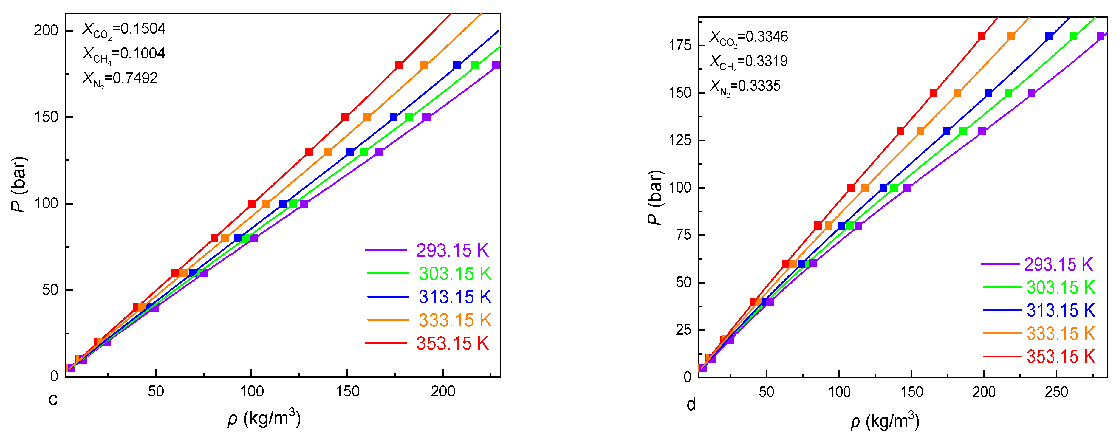
  71. Zhang, Y.; Zhao, B.; Zhao, C.; Zhang, J.; Chen, K.; Xu, Y. Density Characteristics of a Multicomponent CO2/N2/CH4 Ternary Mixture at Temperature of 293.15–353.15 K and Pressure of 0.5–18 MPa. J. Chem. Eng. Data 2022, 67, 908–918. [Google Scholar] [CrossRef]
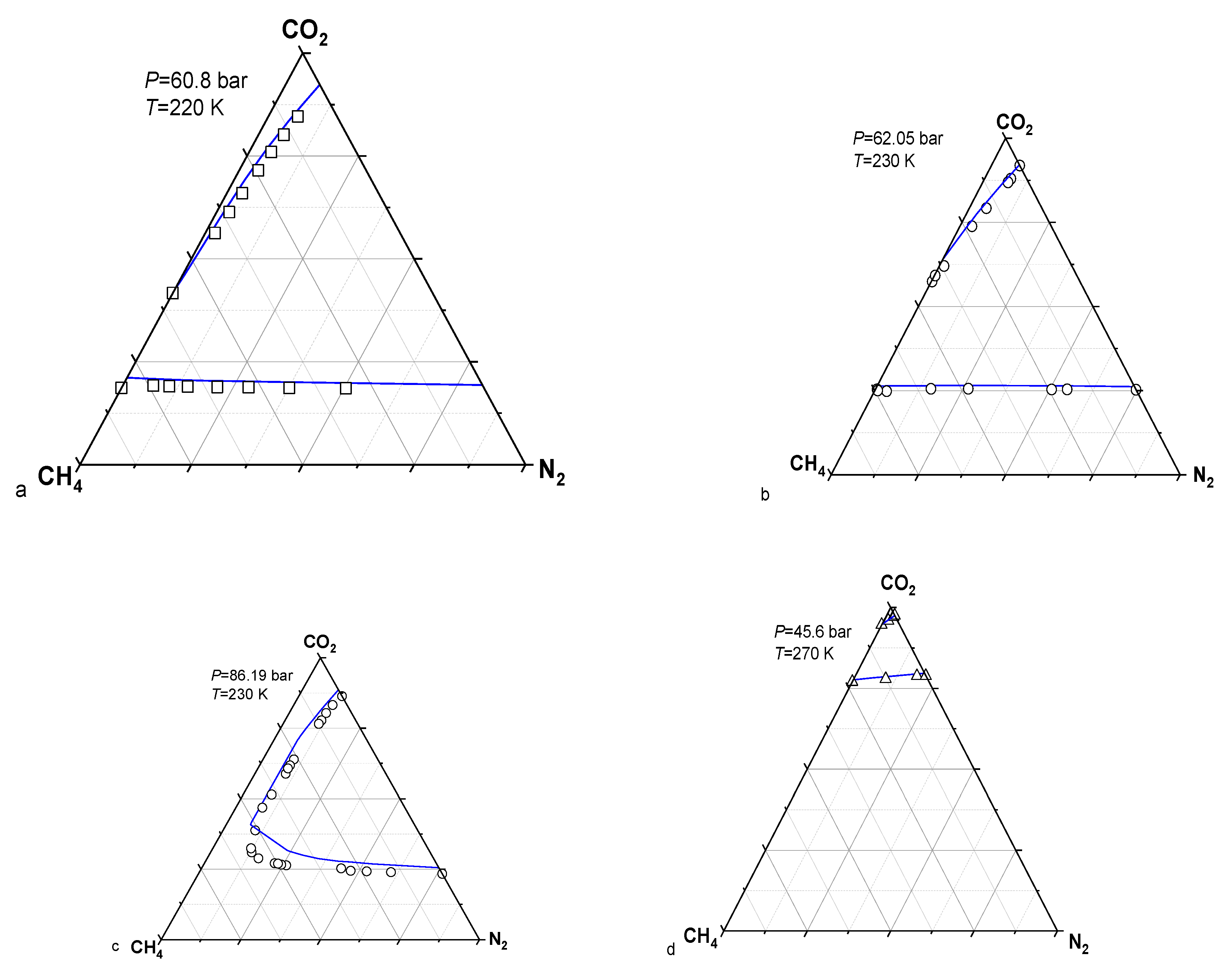
  72. Al-Sahhaf, T.A. Vapor—Liquid equilibria for the ternary system N2+ CO2+ CH4 at 230 and 250 K. Fluid Phase Equilibria 1990, 55, 159–172. [Google Scholar] [CrossRef]
  73. Al-Sahhaf, T.A.; Kidnay, A.J.; Sloan, E.D. Liquid+ vapor equilibriums in the nitrogen+ carbon dioxide+ methane system. Ind. Eng. Chem. Fundam. 1983, 22, 372–380. [Google Scholar] [CrossRef]
  74. Somait, F.A.; Kidnay, A.J. Liquid-vapor equilibriums at 270.00 K for systems containing nitrogen, methane, and carbon dioxide. J. Chem. Eng. Data 1978, 23, 301–305. [Google Scholar] [CrossRef]
  75. Lee, J.; Mather, A. The excess enthalpy of gaseous mixtures of carbon dioxide with methane. Can. J. Chem. Eng. 1972, 50, 95–100. [Google Scholar] [CrossRef]
  76. Lee, J.; Mather, A. The excess enthalpy of gaseous mixtures of nitrogen and carbon dioxide. J. Chem. Thermodyn. 1970, 2, 881–895. [Google Scholar] [CrossRef]
  77. Klein, R.; Bennett, C.; Dodgge, B. Experimental heats of mixing for gaseous nitrogen and methane. AIChE J. 1971, 17, 958–965. [Google Scholar] [CrossRef]
  78. Pitzer, K.S. Thermodynamics of electrolytes. I. Theoretical basis and general equations. J. Phys. Chem. 1973, 77, 268–277. [Google Scholar] [CrossRef] [Green Version]
  79. Akinfiev, N.N.; Diamond, L.W. Thermodynamic model of aqueous CO2–H2O–NaCl solutions from− 22 to 100 °C and from 0.1 to 100 MPa. Fluid Phase Equilibria 2010, 295, 104–124. [Google Scholar] [CrossRef]
  80. Chapoy, A.; Mohammadi, A.; Chareton, A.; Tohidi, B.; Richon, D. Measurement and modeling of gas solubility and literature review of the properties for the carbon dioxide− water system. Ind. Eng. Chem. Res. 2004, 43, 1794–1802. [Google Scholar] [CrossRef]
  81. Chapoy, A.; Mohammadi, A.H.; Richon, D.; Tohidi, B. Gas solubility measurement and modeling for methane–water and methane–ethane–n-butane–water systems at low temperature conditions. Fluid Phase Equilibria 2004, 220, 113–121. [Google Scholar] [CrossRef]
  82. Darwish, N.; Hilal, N. A simple model for the prediction of CO2 solubility in H2O–NaCl system at geological sequestration conditions. Desalination 2010, 260, 114–118. [Google Scholar] [CrossRef]
  83. Duan, Z.; Mao, S. A thermodynamic model for calculating methane solubility, density and gas phase composition of methane-bearing aqueous fluids from 273 to 523 K and from 1 to 2000 bar. Geochim. Cosmochim. Acta 2006, 70, 3369–3386. [Google Scholar] [CrossRef]
  84. Duan, Z.; Sun, R. An improved model calculating CO2 solubility in pure water and aqueous NaCl solutions from 273 to 533 K and from 0 to 2000 bar. Chem. Geol. 2003, 193, 257–271. [Google Scholar] [CrossRef]
  85. Dubessy, J.; Tarantola, A.; Sterpenich, J. Modelling of liquid-vapour equilibria in the H2O-CO2-NaCl and H2O-H2S-NaCl systems to 270 C. Oil Gas Sci. Technol. 2005, 60, 339–355. [Google Scholar] [CrossRef] [Green Version]
  86. Mao, S.; Duan, Z. A thermodynamic model for calculating nitrogen solubility, gas phase composition and density of the N2–H2O–NaCl system. Fluid Phase Equilibria 2006, 248, 103–114. [Google Scholar] [CrossRef]
  87. Portier, S.; Rochelle, C. Modelling CO2 solubility in pure water and NaCl-type waters from 0 to 300 °C and from 1 to 300 bar: Application to the Utsira Formation at Sleipner. Chem. Geol. 2005, 217, 187–199. [Google Scholar] [CrossRef]
  88. Shi, X.; Mao, S. An improved model for CO2 solubility in aqueous electrolyte solution containing Na+, K+, Mg2+, Ca2+, Cl and SO42− under conditions of CO2 capture and sequestration. Chem. Geol. 2017, 463, 12–28. [Google Scholar] [CrossRef]
  89. Søreide, I.; Whitson, C.H. Peng-Robinson predictions for hydrocarbons, CO2, N2, and H2S with pure water and NaCI brine. Fluid Phase Equilibria 1992, 77, 217–240. [Google Scholar] [CrossRef]
  90. Spivey, J.P.; McCain, W.D.; North, R. Estimating density, formation volume factor, compressibility, methane solubility, and viscosity for oilfield brines at temperatures from 0 to 275 °C, pressures to 200 MPa, and salinities to 5.7 mole/kg. J. Can. Pet. Technol. 2004, 43. [Google Scholar] [CrossRef]
  91. Mao, S.; Zhang, D.; Li, Y.; Liu, N. An improved model for calculating CO2 solubility in aqueous NaCl solutions and the application to CO2–H2O–NaCl fluid inclusions. Chem. Geol. 2013, 347, 43–58. [Google Scholar] [CrossRef]
  92. Dhima, A.; de Hemptinne, J.-C.; Jose, J. Solubility of hydrocarbons and CO2 mixtures in water under high pressure. Ind. Eng. Chem. Res. 1999, 38, 3144–3161. [Google Scholar] [CrossRef]
  93. Qin, J.; Rosenbauer, R.J.; Duan, Z. Experimental measurements of vapor–liquid equilibria of the H2O+ CO2+ CH4 ternary system. J. Chem. Eng. Data 2008, 53, 1246–1249. [Google Scholar] [CrossRef]
  94. Liu, Y.; Hou, M.; Ning, H.; Yang, D.; Yang, G.; Han, B. Phase equilibria of CO2+ N2+ H2O and N2+ CO2+ H2O+ NaCl+ KCl+ CaCl2 systems at different temperatures and pressures. J. Chem. Eng. Data 2012, 57, 1928–1932. [Google Scholar] [CrossRef]
Figure 1. Density deviations for the CH4-N2 system at different pressures. Experimental data(triangles [64], stars [52], rounds [54], squares [49]): P is the pressure, ρ cal   is the calculated density, and ρ exp is the experimental density.
Applsci 13 03659 g001
Figure 2. Experimental and calculated densities for the 0.8 mole CH4 + 0.2 mole N2 mixture at different temperatures. The experimental density data (rounds) [68], the PR (green dash lines) and SRK (blue dash lines) EOSs [67], this work (red lines): P is the pressure, ρ   is the density, and T is temperature.
Applsci 13 03659 g002
Figure 3. Vapor-liquid phase equilibria of the CH4-N2 system at different temperatures, (a) P- x N 2 / y N 2 figure at 170 K; (b) P- x CH 4 / y CH 4 figure for 170 K; (c) P- x N 2 / y N 2 figure for 115 K; (d) P- x CH 4 /   y CH 4 figure for 115 K; (e) P- x N 2 / y N 2 figure for 110 K; (f) P- x CH 4 / y CH 4 figure for 110 K. Experimental data (rounds [55], triangles [57], squares [59]), this work (solid lines): x N 2 and y N 2 are the mole fractions of N2 in the liquid and vapor phases, respectively x CH 4 and y CH 4 are the mole fractions of CH4 in the liquid and vapor phases, respectively.
Applsci 13 03659 g003aApplsci 13 03659 g003b
Figure 4. Comparisons between experimental and calculated densities for the CO2-CH4-N2 mixture at different temperatures. (a) X CO 2 = 0.0998 ,   X CH 4 = 0.6625 ,   X N 2 = 0.2477 ;   (b) X CO 2 = 0.9949 ,   X CH 4 = 0.02 ,   X N 2 = 0.0301 ; (c) X CO 2 = 0.1504 ,   X CH 4 = 0.1004 ,   X N 2 = 0.7492 ; (d) X CO 2 = 0.3346 ,   X CH 4 = 0.3319 ,   X N 2 = 0.3335 . Experimental data (squares [71]), this work (solid lines): X CO 2 is the mole fraction of CO2 in the mixture, X CH 4 is the mole fraction of CH4 in the mixture, X N 2 is the mole fraction of N2 in the mixture.
Applsci 13 03659 g004aApplsci 13 03659 g004b
Figure 5. Vapor-liquid phase equilibria for the CO2-CH4-N2 system at different temperatures and pressures, (a) T = 220 K, P = 60.8 bar; (b) T = 230 K, P = 62.05 bar; (c) T = 230 K, P = 86.19 bar; (d) T = 270 K, P = 45.6 bar. Experimental data (squares [73], rounds [72], triangles [74]), this work (solid lines).
Applsci 13 03659 g005
Figure 6. Comparisons between experimental and calculated mixing enthalpies for the CH4-CO2 mixture, (a) T = 283.15 K, P = 10.13bar; (b) T = 283.15 K, P = 30.40 bar; (c) T = 313.15 K, P = 10.13 bar; (d) T = 313.15 K, P = 30.40 bar. Experimental data (squares [75]). PR(kij = 0) (red dash curves); PR (optimal kij) (green dash curves); PR + EOS/ a r e s E , W i l s o n (blue dash curves); This work (black solid curves): h E   is   the mixing enthalpy.
Applsci 13 03659 g006
Figure 7. Comparisons between experimental and calculated mixing enthalpies for the CO2-N2 mixture, (a) T = 313.15 K, P = 10.13bar; (b) T = 313.15 K, P = 30.40 bar; (c) T = 313.15 K, P = 81.06 bar; (d) T = 313.15 K, P = 121.59 bar. Experimental data (black squares [76]). PR (kij = 0) (red dash curves); PR (optimal kij) (green dash curves); PR + EOS/ a r e s E , W i l s o n (blue dash curves); This work (black solid curves).
Applsci 13 03659 g007aApplsci 13 03659 g007b
Figure 8. Comparisons between experimental and calculated mixing enthalpies for the CH4-N2 mixture at 195.15 K and 253.15 K. (a) T = 195.15 K; (b) T = 253.15 K. Experimental data (squares [77]), this work (solid curves); the Enhanced-Predictive-PR78 (E-PPR78) EOS (dash curves).
Applsci 13 03659 g008
Figure 9. Comparisons between experimental and calculated solubilities for the CH4-CO2 mixture in water. (a) m C H 4 - y C H 4 figure at 344.15 K; (b) m C O 2   -   y C H 4   figure at 344.15 K;(c) m C H 4 - y C H 4 figure at 373.5 K; (d) m C O 2   -   y C H 4   figure at 375.5 K; (e) m C H 4 - y C H 4 figure at 324.5 K; (f) m C O 2   -   y C H 4   figure at 324.5 K. Experimental data (rounds [92], squares [93]), this work (solid curves): m C O 2     is the solubility of CO2, m C H 4 is the solubility of CH4.
Applsci 13 03659 g009
Figure 10. Comparisons between experimental and calculated solubilities for the CO2-N2 mixture in water. (a) m N 2   -   y N 2 figure at 308.15 K; (b)   m CO 2 -   y N 2 figure at 308.15 K; (c) m N 2   -   y N 2 figure at 318.15 K; (d) m CO 2 -   y N 2 figure at 318.15 K. Experimental data (squares [94]), this work (solid curves): m N 2   is   the solubility of N2.
Applsci 13 03659 g010
Figure 11. Comparisons between experimental and calculated solubilities for the CO2-N2 mixture in saline water. (a) m N 2   -   y N 2 figure; (b) m CO 2 -   y N 2 figrure. Experimental data (black squares [94]), this work (solid curves).
Applsci 13 03659 g011
Figure 12. Normalized CO2 storage capacity calculated by this EOS of CO2-CH4-N2 mixture. (a) the Normalized capacity-P figure at different temperatures for the same composition; (b) the Normalized capacity-P figure at differents compositions for the same temperatures.
Applsci 13 03659 g012
Figure 13. Calculated isochores of the CO2-CH4-N2 mixture by this EOS, (a) X CO 2 = 0.8 ,   X CH 4 = 0.1 ,   X N 2 = 0.1 ; (b) X CO 2 = 0.7 ,   X CH 4 = 0.15 ,   X N 2 = 0.15 : Vm is the molar volume.
Applsci 13 03659 g013
Table 1. Critical parameters of pure fluids.
Component i T c i   ( K ) ρ c i   ( mol / dm 3 ) References
CH490.694110.139Setzmann and Wagner [42]
CO2216.59210.625Span and Wagner [41]
N263.15111.184Span et al. [43]
Table 2. Binary interaction parameters of the CO2-CH4-N2 system.
ReferencesBinary Mixtures F i j ζ i j   ( dm 3 / mol ) ς i j   ( K ) β i j
Mao et al. [40]CH4-CO20.12844025 × 100.35751245 × 10−2−0.43720344 × 1020.10358865 × 10
Zhang et al. [34]CO2-N20.16671494 × 100.58411078 × 10−2−0.22952094 × 1020.16878787 × 10
This workCH4-N20.637399970.3812517 × 10−2−0.17790001 × 1020.1009001 × 10
Note: Subscripts i and j refer to the first component and the second component, respectively.
Table 3. Calculated PVTx and VLE deviations for the CH4-N2 mixture.
ReferencesNumber of Data PointsT-P-x Range for xCH4-(1-x) N2AAD%
StylesTotal (Used)T (K)P (bar)x
Liu and Miller [45]PVTx7 (0)91–1153–120.50.57
Rodosevich and Miller [46]PVTx8 (0)91–11543–4540.8–0.953.83
Pan et al. [47]PVTx7 (0)91–1151–110.5–0.860.11
Hiza et al. [48]PVTx21 (0)95–1401–210.5–0.950.10
Da Ponte et al. [49]PVTx182 (50)110–12015–13800.3–0.680.12
Straty and Diller [65]PVTx578 (0)82–3206–3560.32–0.70.24
Haynes and McCarty [56]PVTx85 (85)140–32010–1640.3–0.710.09
Seitz et al. [64]PVTx190 (90)323–57399–9990.1–0.90.28
Seitz and Blencoe [63]PVTx43 (0)673.15199–9990.1–0.95.36
Ababio et al. [50]PVTx83 (83)308–3339–1200.5–0.780.12
Chamorro et al. [52]PVTx242 (56)230–4009–1920.8–0.90.23
Janisch et al. [57]PVTx17 (0)129–18015–500.4–0.92.10
Li et al. [60]PVTx27 (27)17–2701–160.90.06
Gomez-Osorio et al. [54]PVTx142 (42)304–470100–13790.25–0.750.07
Brandt and Stroud [51]VLE23 (0)128–179340.05–0.981.48
Cheung and Wang [53]VLE20 (0)92–1240.2–60.85–1.05.02
Pan et al. [47]VLE60 (60)95–1200.2–250.05–15.05
Miller et al. [62]VLE11 (0)1122–130.2–0.973.30
Kidnay et al. [59]VLE83 (83)112–1802–490.1–0.991.31
McClure et al. [61]VLE8 (8)911–30.1–0.85.60
Jin et al. [58]VLE10 (10)1234–260.1–0.952.96
Parrish and Hiza [66]VLE48 (43)95–1202–200.1–0.93.14
Janisch et al. [57]VLE16 (6)130–1800.5–50.4–0.961.14
Han et al. [55]VLE77 (60)110–1234–130.7–1.02.49
Note: Deviations of the PVTx data are the density deviations, and the deviations of VLE data are the equilibrium composition deviations. AAD is the abbreviation of average absolute deviation.
Table 4. Calculated PVTx deviations for the ternary CO2-CH4-N2 mixture.
ReferencesNT-P-x Range for xCO2-yCH4-(1-x-y) N2AAD%
T (K)P (bar)xy
McElroy et al. [59]242303–3336–1260–0.99980–0.9990.45
Seitz et al. [60]42474.1510000.0–1.00.0–1.00.28
Seitz et al. [55]271323–573199–9990.1–0.80.1–0.80.28
Zhang et al. [61]200293.15–353.255–1800.098–0.99490.02–0.65250.52
Le et al. [1]84305.155–6000.499–0.8990.0505–0.3310.82
Note: Deviations of the PVTx data are the density deviations. N is the Number of data points, AAD is the abbreviation of average absolute deviation.
Table 5. Ranges of pure gas solubility models.
Pure GasTP Salinity   ( m NaCl ) References
CH4273–523 K1–2000 bar0–6 mol/kgDuan and Mao [83]
CO2273.15–723.15 K1–1500 bar0–4.5 mol/kgMao et al. [91]
N2273–590 K1–600 bar0–6 mol/kgMao and Duan [86]
Disclaimer/Publisher’s Note: The statements, opinions and data contained in all publications are solely those of the individual author(s) and contributor(s) and not of MDPI and/or the editor(s). MDPI and/or the editor(s) disclaim responsibility for any injury to people or property resulting from any ideas, methods, instructions or products referred to in the content.

