
The Influence of the Magnetic Field Line Curvature on Wall Erosion near the Hall Thruster Exit Plane

Abstract
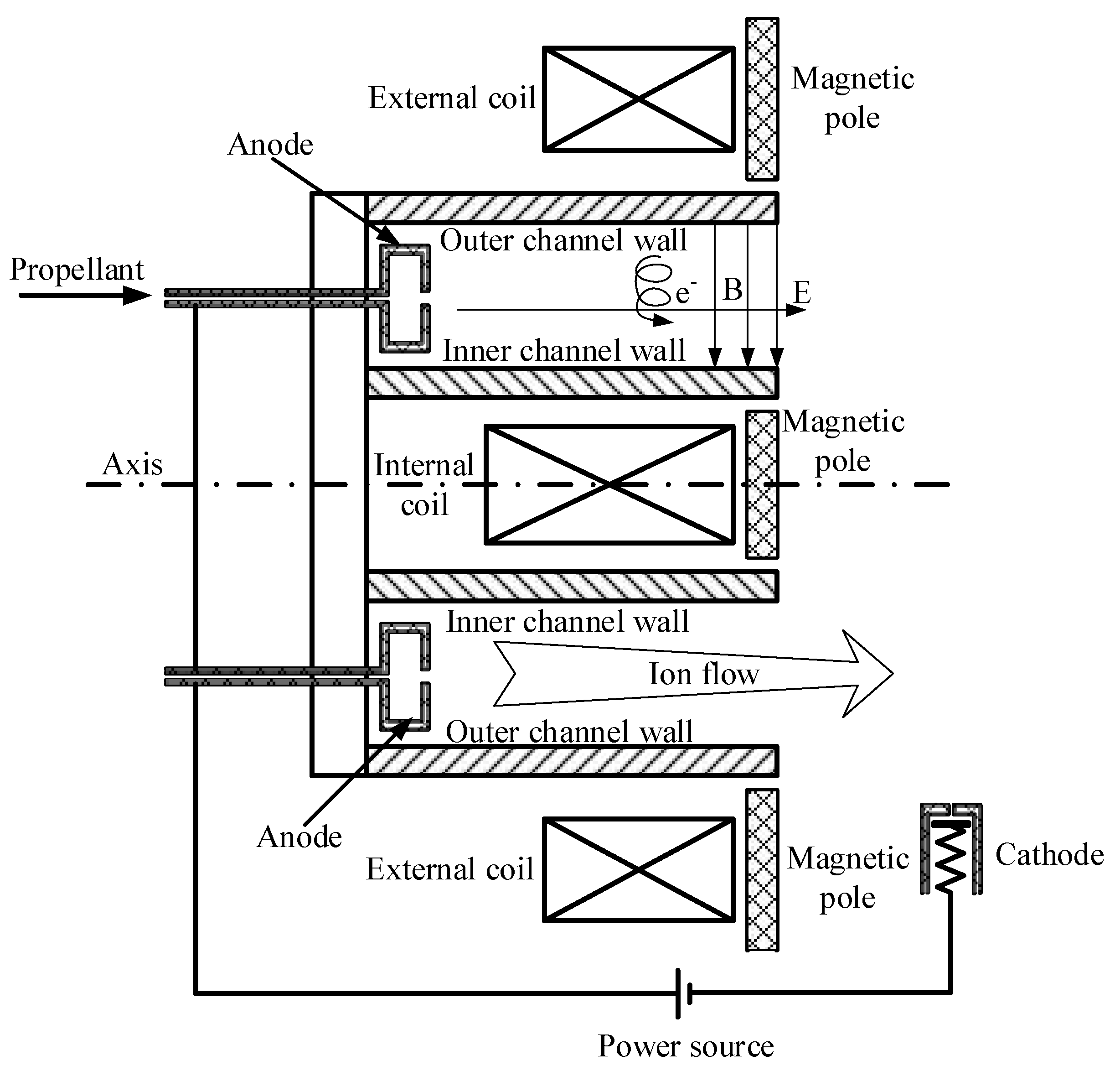
:1. Introduction
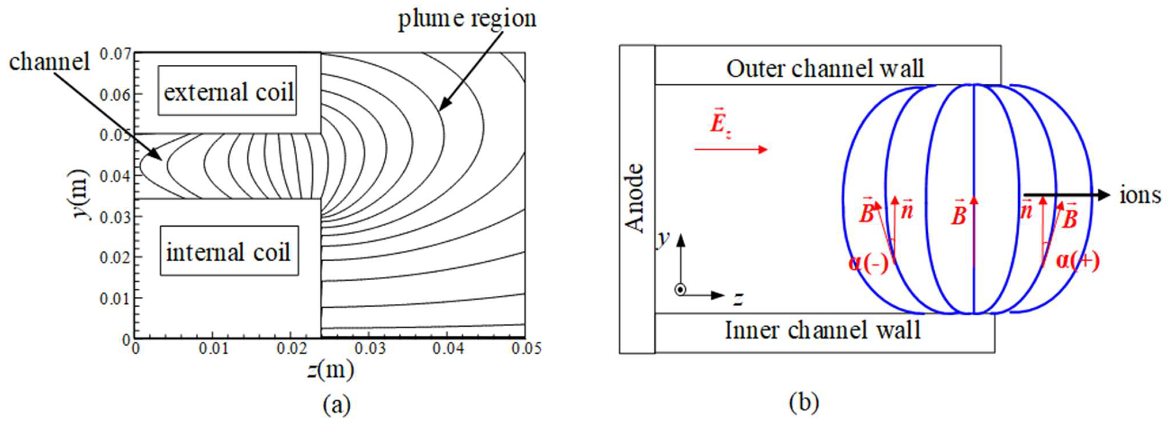
2. Theory and Calculation Model
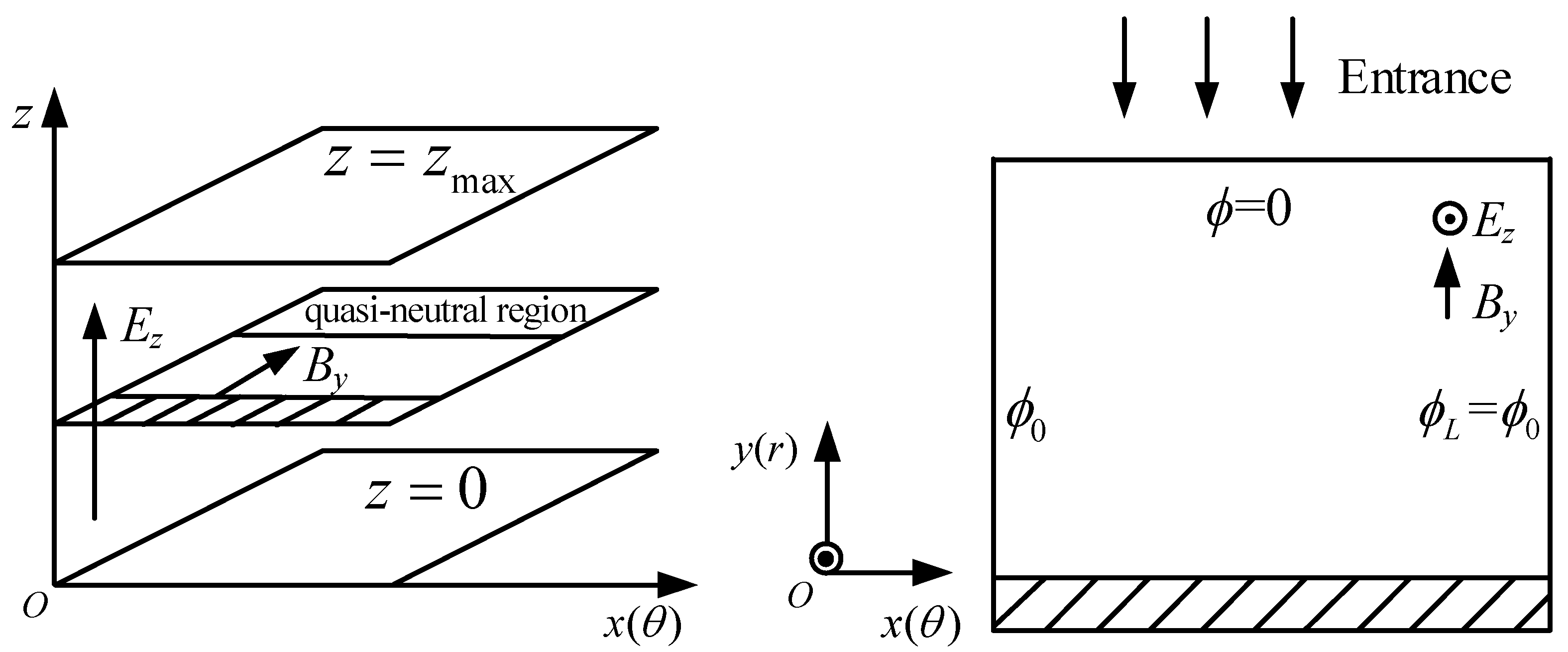
2.1. PIC Simulation Model
2.2. Model Settings
2.3. Sputtering Model
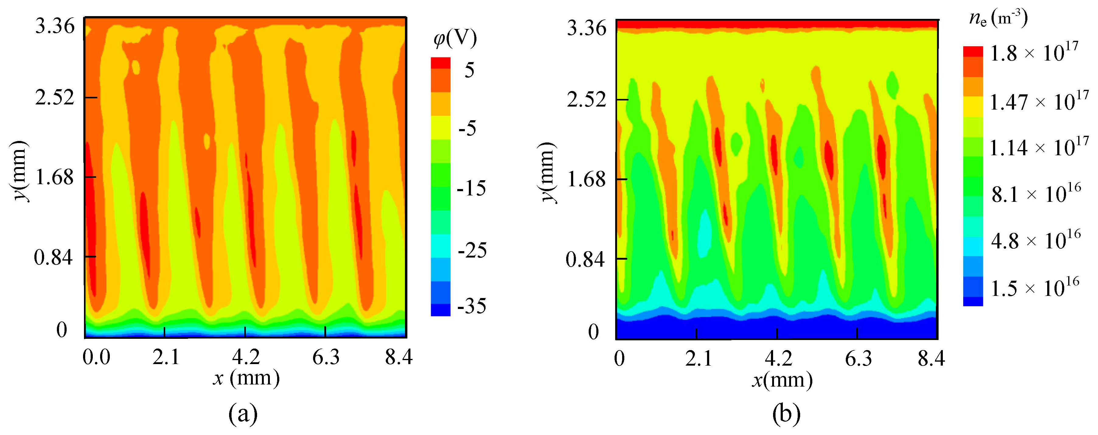
3. Results and Discussions
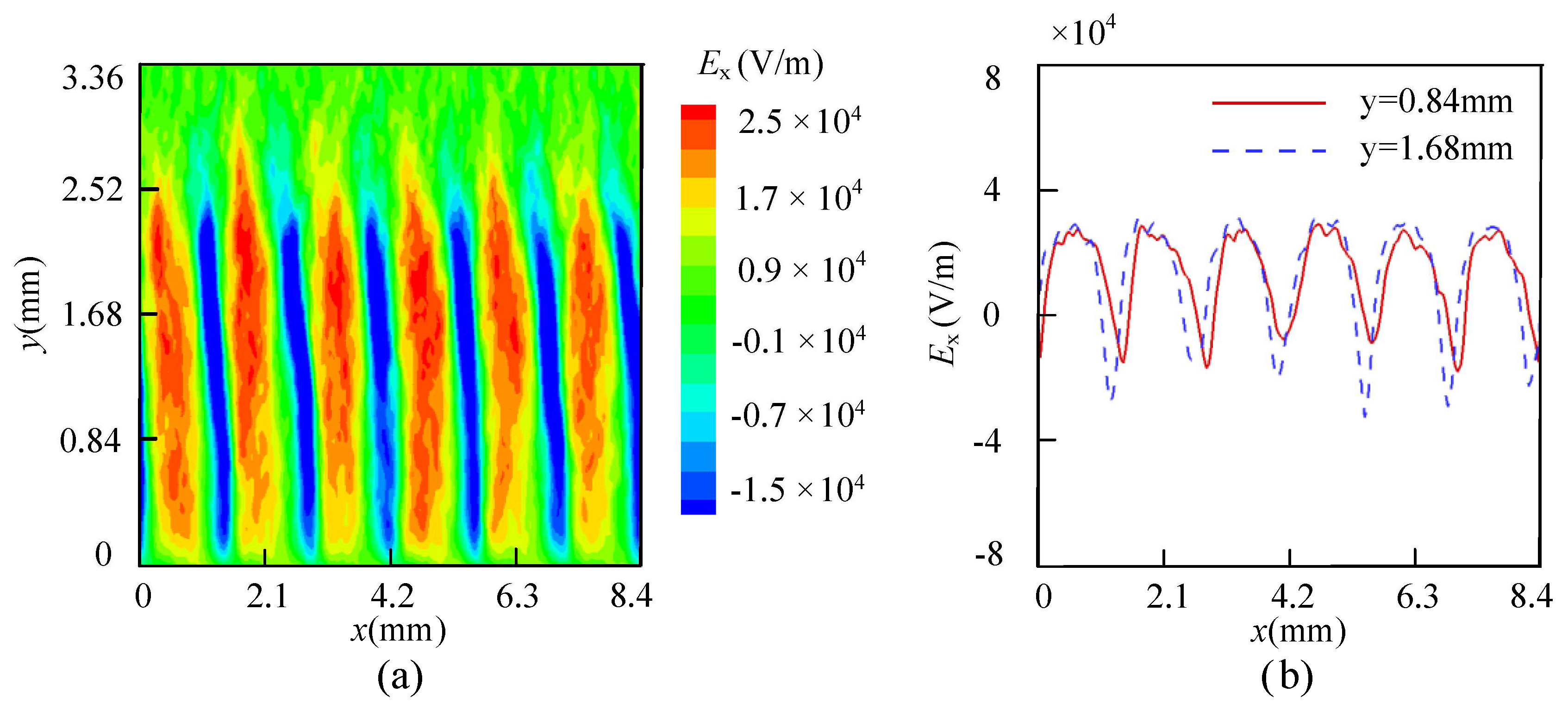
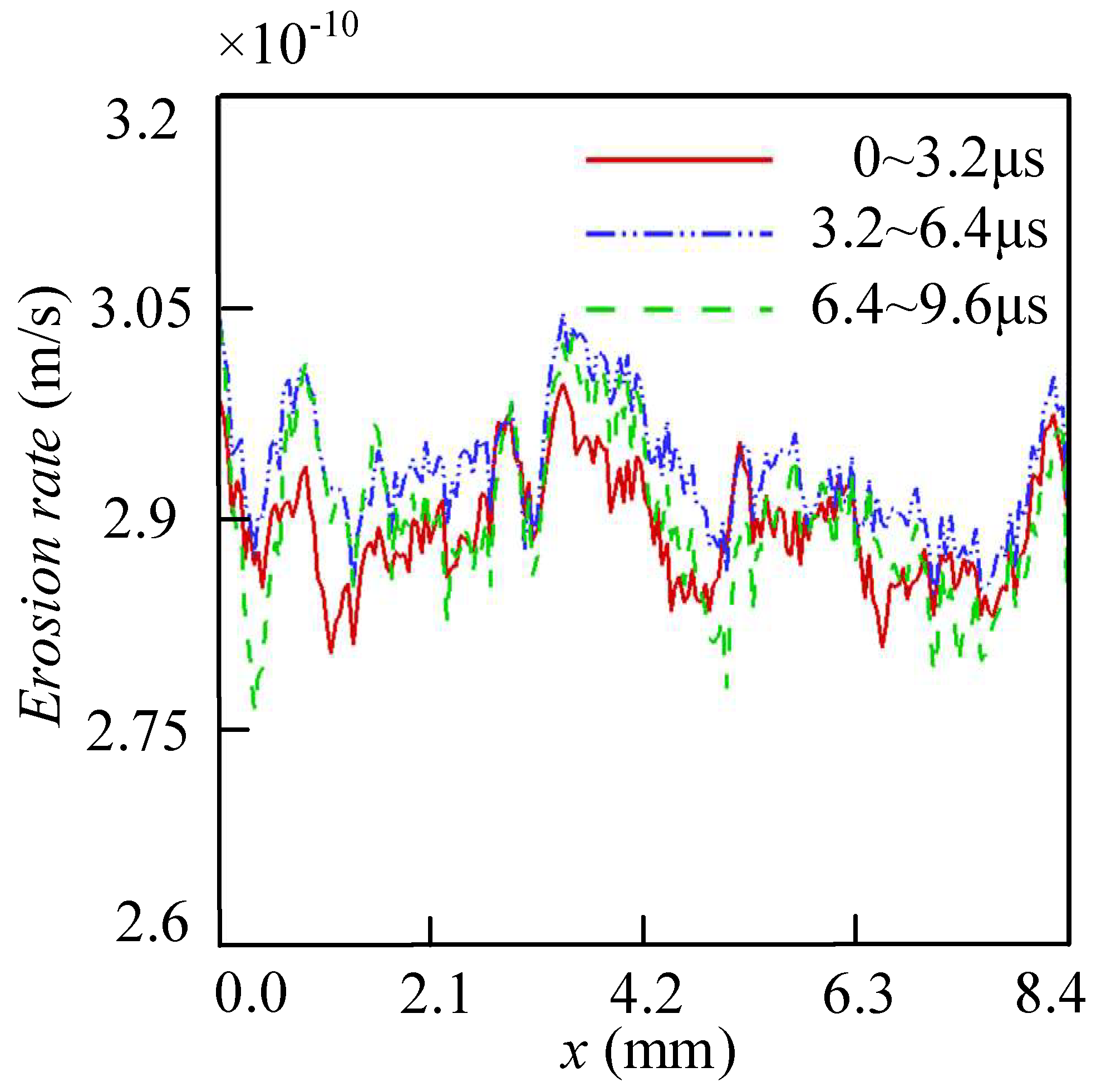
3.1. Wall Erosion When the Value of α Is 0
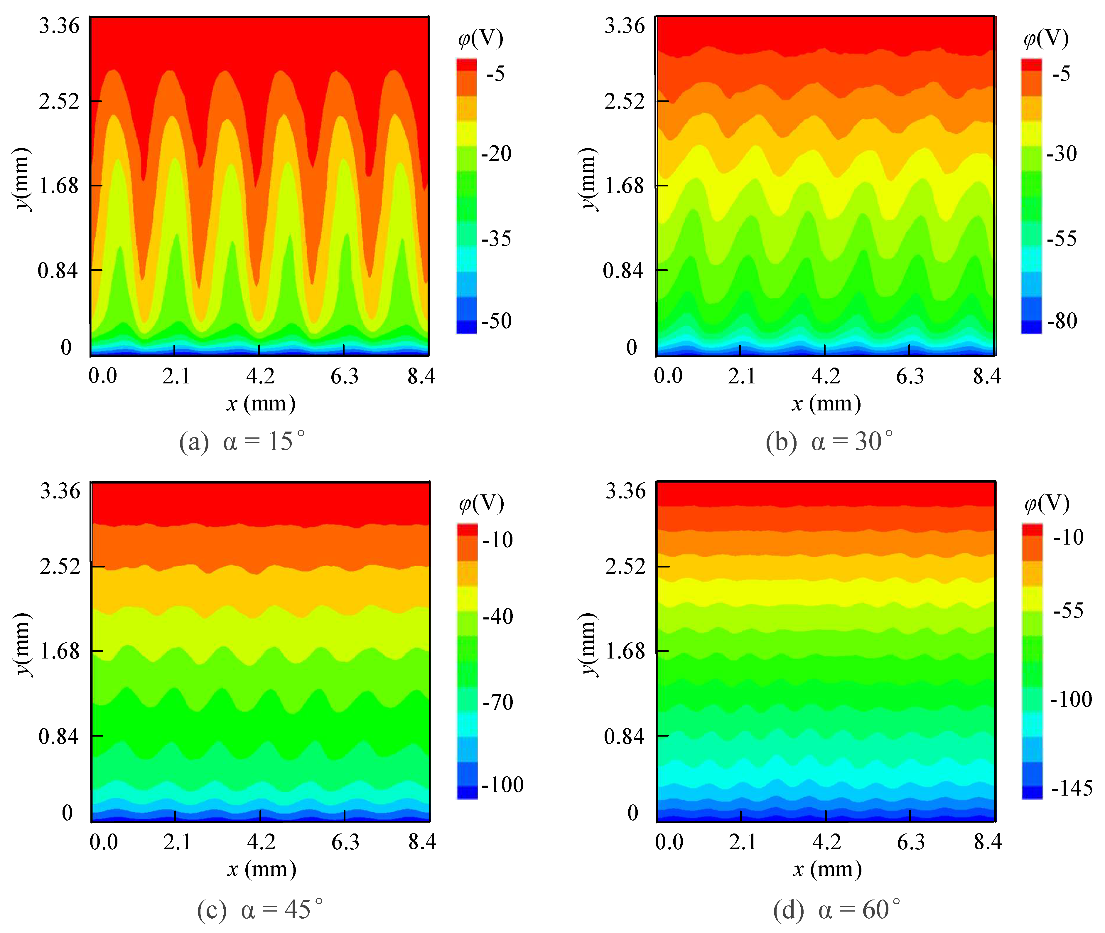
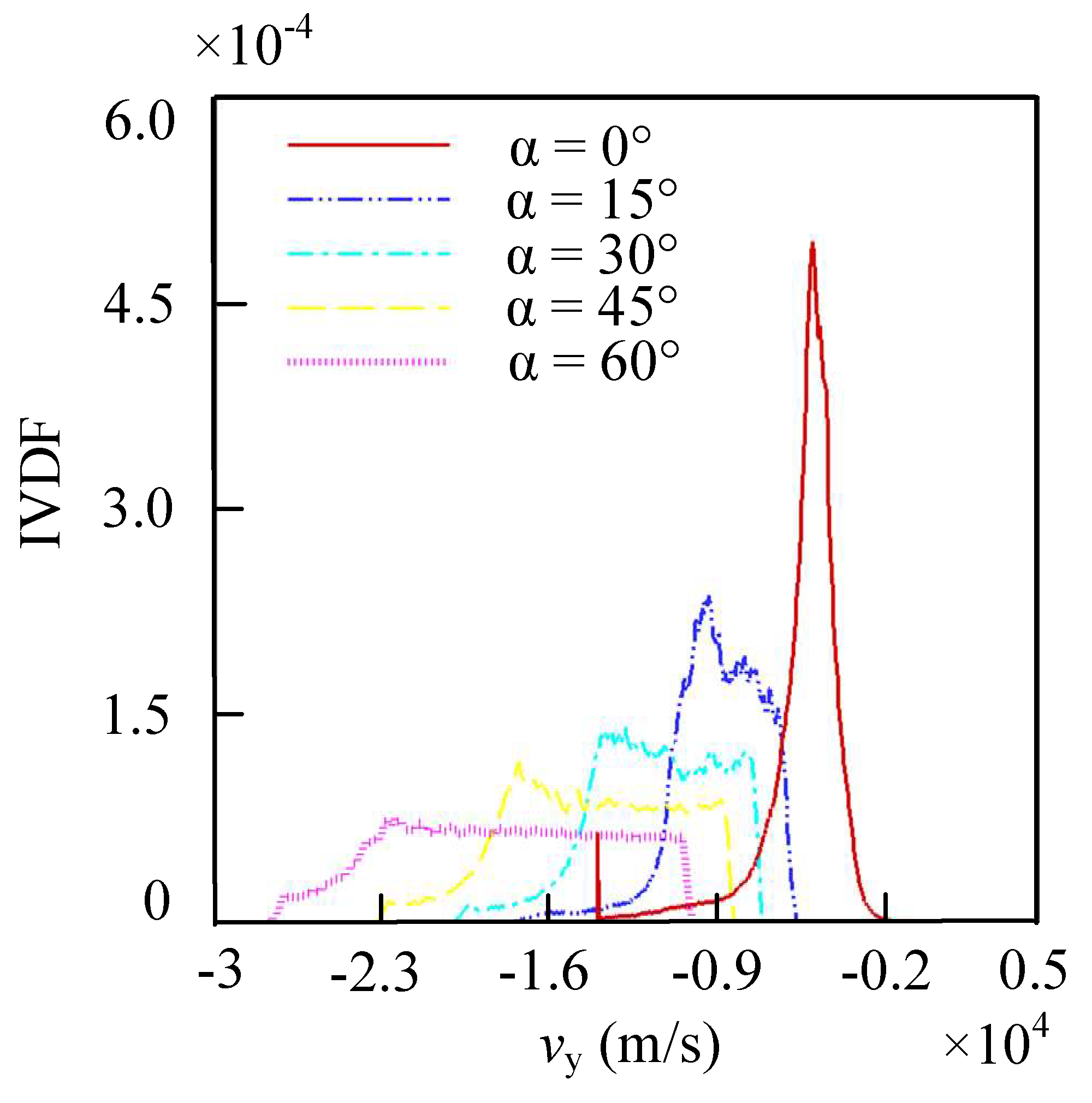
3.2. Wall Erosion When the Value of α Is Positive
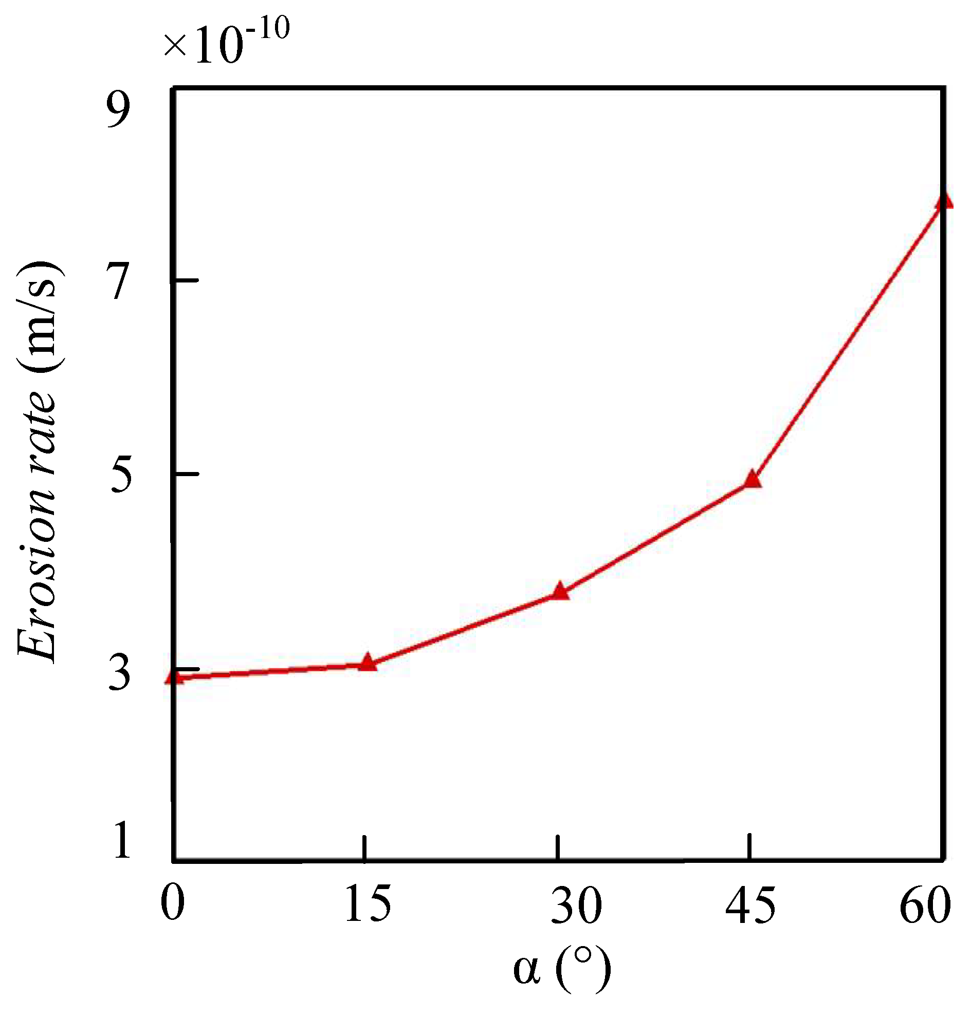
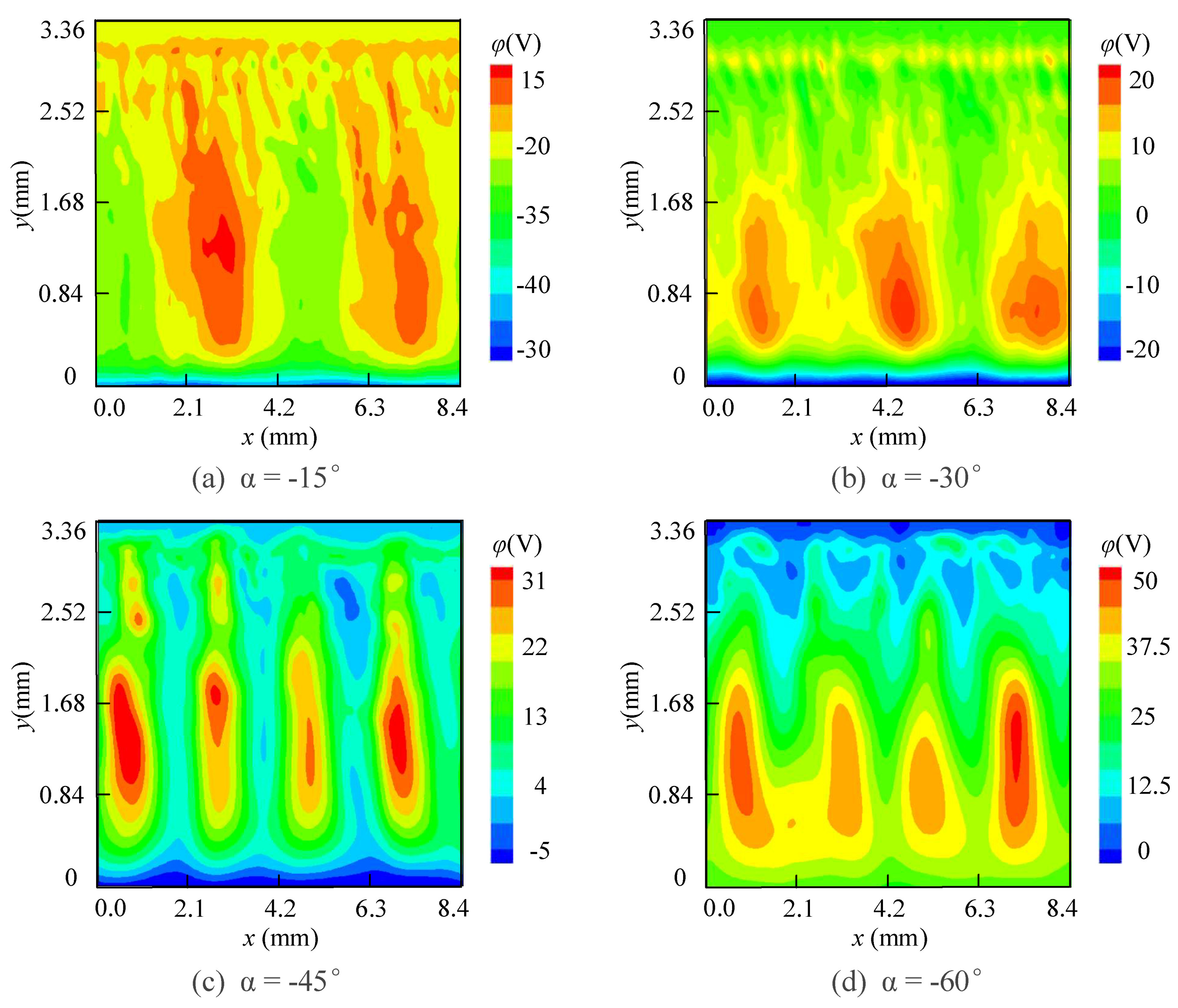
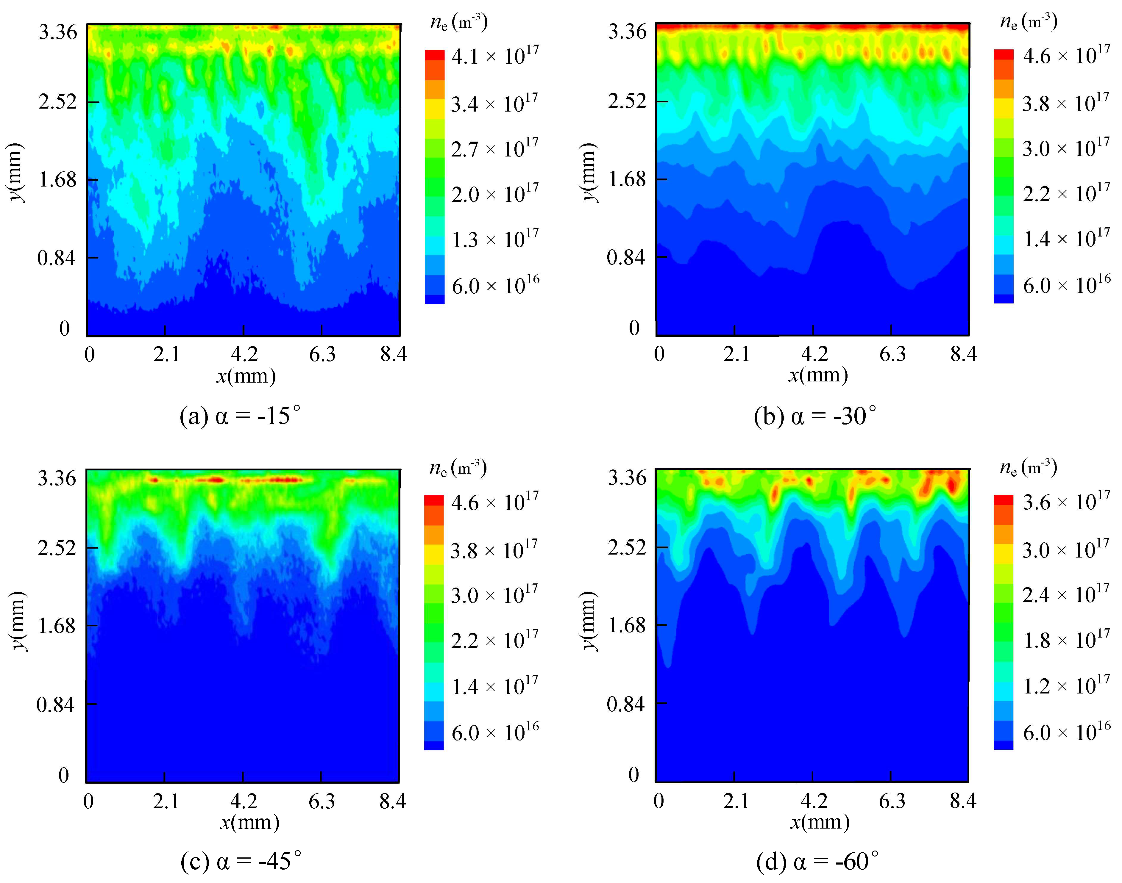
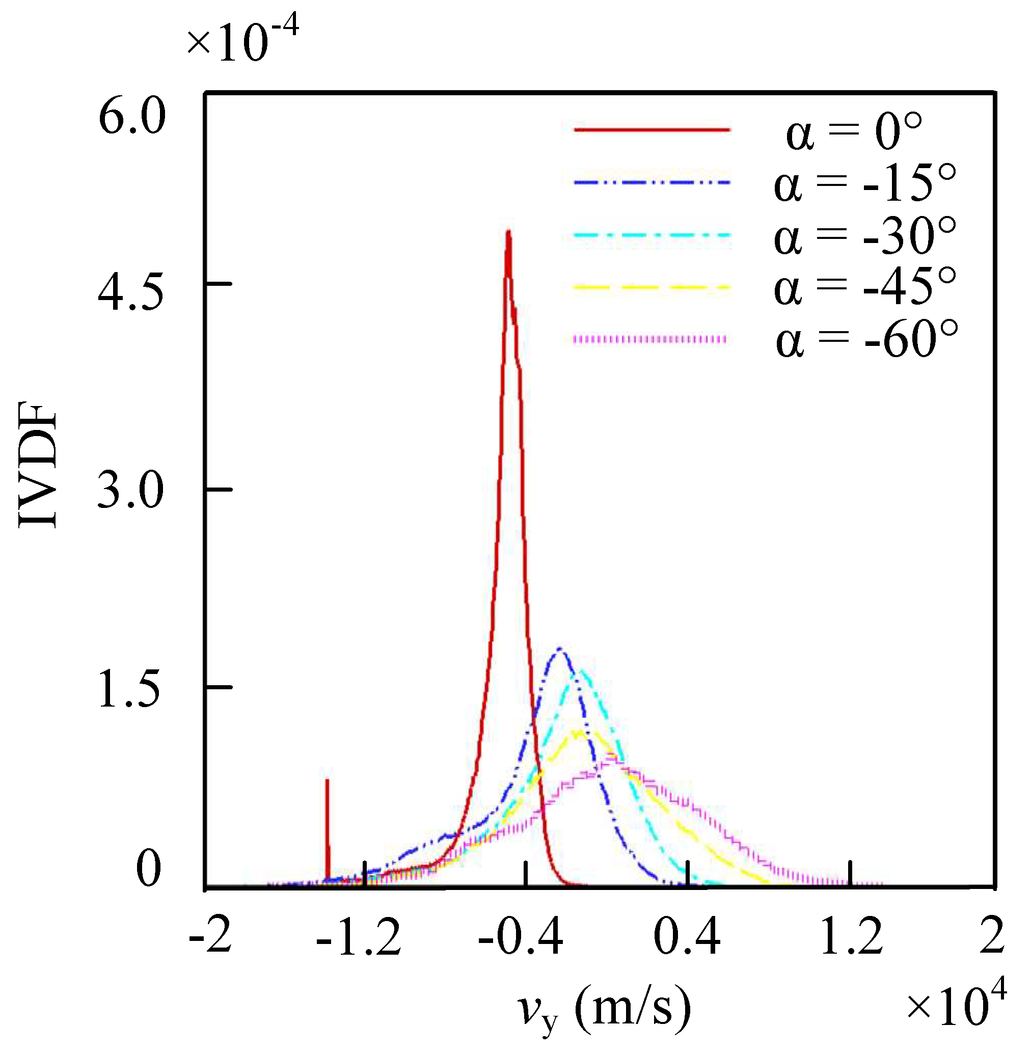
3.3. Wall Erosion under Negative α
4. Conclusions
Author Contributions
Funding
Institutional Review Board Statement
Informed Consent Statement
Data Availability Statement
Conflicts of Interest
Nomenclature
| B | Magnetic field, T |
| Bz | axial magnetic field, T |
| By | radial magnetic field, T |
| e | elementary charge, C |
| E | electric field, V/m |
| Ez | axial electric field, V/m |
| Ex | azimuthal electric field, V/m |
| oscillating azimuthal electric field, V/m | |
| Eth | sputtering threshold, eV |
| En | Sputtering energy, eV |
| J | flux density, m−2·s−1 |
| Lx | azimuthal domain length, m |
| Ly | radial domain length, m |
| Lz | axial domain length, m |
| me | Electron mass, kg |
| mi | ion mass, kg |
| n0 | Ion density in quasineutral region, m−3 |
| ne | Electron density in simulation, m−3 |
| ni | Ion density in simulation, m−3 |
| Np | Number of particles per cell |
| N | atomic density, Kg/m3 |
| q | erosion rate, m/s |
| R | Simulation domain, m3 |
| S | ion energy sputtering coefficient |
| Δt | time step, s |
| Te | electron temperature, eV |
| v | velocity, m/s |
| Δx | grid spacing, m |
| Y | sputtering yield |
| Y’ | ion incident angle dependent sputtering yield |
| Greek | |
| 𝛼 | tilt angle of magnetic line, ° |
| 𝜖 | vacuum permittivity, F/m |
| λDe | Debye length, m |
| Φ | Electric potential, V |
| 𝜃 | Ion incidence angle, ° |
| Subscripts | |
| e | electronic |
| i | ionic |
| ωpe | electron plasma frequency, rad/s |
| x | Azimuth direction |
| y | Radial direction |
| z | Axial direction |
References
- Goebel, D.M.; Katz, I. Fundamentals of Electric Propulsion: Ion and Hall Thrusters; John Wiley & Son Inc.: Hoboken, NJ, USA, 2008; pp. 325–389. [Google Scholar]
- Oleson, S.R.; Myers, R.M.; Kluever, C.A. Advanced Propulsion for Geostationary Orbit Insertion and North-South Station Keeping. J. Spacecr. Rockets 1997, 34, 22–28. [Google Scholar] [CrossRef] [Green Version]
- Levchenko, I.; Xu, S.; Mazouffre, S.; Lev, D.; Pedrini, D.; Goebel, D.; Garrigues, L.; Taccogna, F.; Bazaka, K. Perspectives, frontiers, and new horizons for plasma-based space electric propulsion. Phys. Plasmas 2020, 27, 020601-1–020601-30. [Google Scholar] [CrossRef] [Green Version]
- Kim, V. Main Physical Features and Processes Determining the Performance of Stationary Plasma Thrusters. J. Propuls. Power 1998, 14, 736–743. [Google Scholar] [CrossRef] [Green Version]
- Mazouffre, S.; Dubois, F.; Albarede, L.; Pagnon, D.; Touzeau, M.; Dudeck, M. Plasma induced erosion phenomena in a Hall thruster. In Proceedings of the International Conference on Recent Advances in Space Technologies, Istanbul, Turkey, 20–22 November 2003. [Google Scholar]
- Cho, S.; Yokota, S.; Komurasaki, K.; Arakawa, Y. Multilayer coating method for investigating channel-wall erosion in a Hall thruster. J. Propuls. Power 2013, 29, 278–282. [Google Scholar] [CrossRef]
- Pérez-Grande, D.; Fajardo, P.; Ahedo, E. Evaluation of Erosion Reduction Mechanisms in Hall Eect Thrusters. In Proceedings of the 34th International Electric Propulsion Conference, Hyogo-Kobe, Japan, 4–10 July 2015. [Google Scholar]
- Morozov, A.I.; Bugrova, A.I.; Desyatskov, A.V.; Ermakov, Y.A.; Kozintseve, M.V.; Lipatov, A.S.; Pushkin, A.A.; Khartchevnikov, V.K.; Churbanov, D.V. ATON-thruster plasma accelerator. In Proceedings of the Fourth All-Russian Seminar on Problems of Theoretical and Applied Electron Optics, Moscow, Russia, 21–22 October 1999; Volume 23, pp. 587–597. [Google Scholar]
- Brieda, L.; Pai, S.; Dachman, Y.; Keidar, M. Wall Interaction in Hall thrusters with Magnetic Lens Configuration. In Proceedings of the 47th AIAA/ASME/SAE/ASEE Joint Propulsion Conference & Exhibit, San Diego, CA, USA, 31 July–3 August 2011. [Google Scholar]
- Keidar, M.; Boyd, I.D. Effect of a magnetic field on the plasma plume from Hall thrusters. J. Appl. Phys. 1999, 86, 4786–4791. [Google Scholar] [CrossRef]
- Hofer, R.R.; Jankovsky, R.S. The Influence of Current Density and Magnetic Field Topography in Optimizing the Performance, Divergence, and Plasma Oscillations of High Specific Impulse Hall Thrusters. In Proceedings of the 28th International Electric Propulsion Conference, Toulouse, France, 17–21 March 2003. [Google Scholar]
- Hofer, R.R.; Gallimore, A.D. The Role of Magnetic Field Topography in Improving the Performance of a High Voltage Hall Thruster. In Proceedings of the 38th AIAA/ASME/SAE/ASEE Joint Propulsion Conference & Exhibit, Indianapolis, IN, USA, 7–10 July 2002. [Google Scholar]
- Fruchtman, A.; Cohen-Zur, A. Plasma lens and plume divergence in the Hall thruster. Appl. Phys. Lett. 2006, 89, 111501-1–111501-3. [Google Scholar] [CrossRef]
- Garrigues, L.; Hagelaar, G.; Bareilles, J.; Boniface, C.; Boeuf, J.P. Model study of the influence of the magnetic field configuration on the performance and lifetime of a Hall thruster. Phys. Plasmas 2003, 10, 4886–4892. [Google Scholar] [CrossRef]
- Liu, C.; Gu, Z.; Xie, K.; Sun, Y.; Tang, H. Influence of the Magnetic Field Topology on Hall Thruster Discharge Channel Wall Erosion. IEEE Trans. Appl. Supercond. 2012, 22, 4904105. [Google Scholar]
- Liu, J.; Li, H.; Hu, Y.; Liu, X.; Ding, Y.; Wei, L.; Yu, D.; Wang, X. Particle-in-cell simulation of the effect of curved magnetic field on wall bombardment and erosion in a hall thruster. Contrib. Plasma Phys. 2019, 59, e201800001. [Google Scholar] [CrossRef]
- Yu, D.; Zhang, F.; Liu, H.; Li, H.; Yan, G.; Liu, J. Effect of electron temperature on dynamic characteristics of two-dimensional sheath in Hall thrusters. Phys. Plasmas 2008, 15, 104501-1–104501-3. [Google Scholar] [CrossRef]
- Wang, J.J.; Yong, C.; Kafafy, R.; Martinez, R.; Williams, L. Numerical and Experimental Investigations of Crossover Ion Impingement for Subscale Ion Optics. J. Propuls. Power 2015, 24, 562–570. [Google Scholar] [CrossRef]
- Han, D.; Wang, J.; He, X. A Nonhomogeneous Immersed-Finite-Element Particle-in-Cell Method for Modeling Dielectric Surface Charging in Plasmas. IEEE Trans. Plasma Sci. 2016, 44, 1326–1332. [Google Scholar] [CrossRef]
- Lafleur, T.; Chabert, P. The role of instability-enhanced friction on ‘anomalous’ electron and ion transport in Hall-effect thrusters. Plasma Sources Sci. Technol. 2017, 27, 015003-1–015003-19. [Google Scholar] [CrossRef]
- Bai, J.; Cao, Y.; He, X.; Peng, E. An implicit particle-in-cell model based on anisotropic immersed-finite-element method. Comput. Phys. Commun. 2021, 261, 107655-1–107655-11. [Google Scholar] [CrossRef]
- Yu, D.; Li, Y. Volumetric erosion rate reduction of Hall thruster channel wall during ion sputtering process. J. Phys. D Appl. Phys. 2007, 40, 2526–2532. [Google Scholar] [CrossRef]
- Peter, S. Theory of Sputtering. I. Sputtering Yield of Amorphous and Polycrystalline Targets. Phys. Rev. 1969, 184, 383–416. [Google Scholar]
- Yamamura, Y.; Tawara, H. Energy dependence of ion-induced sputtering yields from monatomic solids at normal incidence. At. Data Nucl. Data Tables 1996, 62, 149–253. [Google Scholar] [CrossRef]
- Seah, M. An accurate semi-empirical equation for sputtering yields, II: For neon, argon and xenon ions. Nucl. Instrum. Methods Phys. Res. B 2005, 229, 348–358. [Google Scholar] [CrossRef]
- Yamamura, Y. An empirical formula for angular dependence of sputtering yields. Radiat. Eff. 1984, 80, 57–72. [Google Scholar] [CrossRef]
- Lafleur, T.; Baalrud, S.D.; Chabert, P. Characteristics and transport effects of the electron drift instability in Hall-effect thrusters. Plasma Sources Sci. Technol. 2017, 26, 024008-1–024008-14. [Google Scholar] [CrossRef] [Green Version]


| Symbol | Parameter | Value |
|---|---|---|
| electronic quality | 9.109 × 10⁻³¹ kg | |
| ion mass | 6.63 × 10⁻²⁶ kg | |
| area size | 8.4 mm × 3.36 mm × 8.4 mm | |
| grid length | 4.2 × 10⁻⁵ m | |
| Time Step | 6.4 × 10⁻¹² s | |
| Electric field | 2 × 10⁴ V/m | |
| Magnetic induction | 0.03 T | |
| Ion density in quasi-neutral region | n0 | 2.5 × 10¹⁷/m3 |
| Number of particles per cell | 100 | |
| electron temperature | 10 eV | |
| Electronic Debye length | 4.2 × 10⁻⁵ m |
Disclaimer/Publisher’s Note: The statements, opinions and data contained in all publications are solely those of the individual author(s) and contributor(s) and not of MDPI and/or the editor(s). MDPI and/or the editor(s) disclaim responsibility for any injury to people or property resulting from any ideas, methods, instructions or products referred to in the content. |
© 2023 by the authors. Licensee MDPI, Basel, Switzerland. This article is an open access article distributed under the terms and conditions of the Creative Commons Attribution (CC BY) license (https://creativecommons.org/licenses/by/4.0/).
Share and Cite
Quan, L.; Cao, Y.; Tian, B.; Gong, K. The Influence of the Magnetic Field Line Curvature on Wall Erosion near the Hall Thruster Exit Plane. Appl. Sci. 2023, 13, 3547. https://doi.org/10.3390/app13063547
Quan L, Cao Y, Tian B, Gong K. The Influence of the Magnetic Field Line Curvature on Wall Erosion near the Hall Thruster Exit Plane. Applied Sciences. 2023; 13(6):3547. https://doi.org/10.3390/app13063547
Chicago/Turabian StyleQuan, Lulu, Yong Cao, Bin Tian, and Keyu Gong. 2023. "The Influence of the Magnetic Field Line Curvature on Wall Erosion near the Hall Thruster Exit Plane" Applied Sciences 13, no. 6: 3547. https://doi.org/10.3390/app13063547