Classification of Mineral Foam Flotation Conditions Based on Multi-Modality Image Fusion

Abstract

Accurate and rapid identification of mineral foam flotation states can increase mineral utilization and reduce the consumption of reagents. The traditional flotation process concentrates on extracting foam features from a single-modality foam image, and the accuracy is undesirable once problems such as insufficient image clarity or poor foam boundaries are encountered. In this work, a classification method based on multi-modality image fusion and CNN-PCA-SVM is proposed for work condition recognition of visible and infrared gray foam images. Specifically, the visible and infrared gray images are fused in the non-subsampled shearlet transform (NSST) domain using the parameter adaptive pulse coupled neural network (PAPCNN) method and the image quality detection method for high and low frequencies, respectively. The convolution neural network (CNN) is used as a trainable feature extractor to process the fused foam images, the principal component analysis (PCA) reduces feature data, and the support vector machine (SVM) is used as a recognizer to classify the foam flotation condition. After experiments, this model can fuse the foam images and recognize the flotation condition classification with high accuracy.

1. Introduction

Mineral foam flotation is a beneficiation method used to obtain high-quality minerals. The traditional mining industry has been relying on manual observation of foam to monitor the flotation production conditions, which is subjective and inefficient. Therefore, the use of machine learning for foam flotation work classification is gradually becoming a research hotspot [1]. Oktaba et al. [2] first used an image algorithm to predict the copper content in the foam. Lu et al. [3] proposed a flotation foam size distribution feature extraction approach. Li et al. [4] proposed a floatation detection based on deep learning and a support vector machine. Sameer H. Morar et al. [5] proposed a machine vision technique to measure the rate at which lamellae on the froth surface burst. Zhang et al. [6] proposed a flotation dosing state recognition method based on multiscale CNN features and a ranks automatic encoder kernel extreme learning machine. In the above studies, although machine learning was used to process clear mineral foam images, problems such as insufficient clarity of foam images and poor foam boundaries were ignored. Infrared gray images are less susceptible to interference from complex conditions such as light and smoke but have disadvantages such as inconspicuous details and poor visibility. Visible images can capture a wealth of detailed information. Infrared and visible images present features that are inherent to almost all objects [7]. If these two modality images are used directly, a large amount of redundant information will be generated, which is not conducive to the subsequent work. Due to the ubiquitous and complementary characteristics of infrared and visible images, their fusion technology has solved the above problems and has been widely used. Remote sensing [8], object recognition [7,9], detection [10], and surveillance [11] are classical applications of infrared and visible image fusion. Therefore, in this paper, infrared and visible image fusion techniques are used to process foam images.

In the past few decades, multiscale transformation (MST) has achieved success in areas such as infrared and visible image fusion and is the most active area in image fusion [4]. Generally, MST-based fusion methods include three basic steps. Firstly, the source image is decomposed to obtain low and high-frequency information. Secondly, the low-frequency and high-frequency information is fused according to the corresponding fusion rules. Finally, the fused high and low-frequency bands are used to perform the corresponding inverse transform to obtain the final fused image. The commonly used MST methods in image fusion include Laplace Pyramid (LP) [12], Wavelet Transform [13], Contourlet Transform [14], Non-subsampled Contourlet Transform (NSCT) [15], and Non-subsampled Shearlet Transform (NSST) [16], among which NSST has a great advantage of no direction number limitation and avoiding the Pseudo-Gibbs effect. In addition to the image transform selection, the high and low-frequency coefficient fusion strategy is also a key issue. The high frequency is usually chosen to fuse the maximum absolute value and the simple rule of sampling the weighted average of the low frequency to obtain the fusion coefficients [12]. Since most of the image energy is in the low-frequency sub-bands, the average fusion will reduce the contrast and lose the energy information of the source image. In this paper, the pulse-coupled neural network algorithm (PCNN) is used for high-frequency fusion, and the PCNN is a biological neural network derived from the cortical model of Echorn et al. [17], which has features such as global coupling and pulse synchronization and is well suited as a tool for image fusion. Specifically, PCNN is usually used to extract the activity level of the decomposition coefficients of the MST. 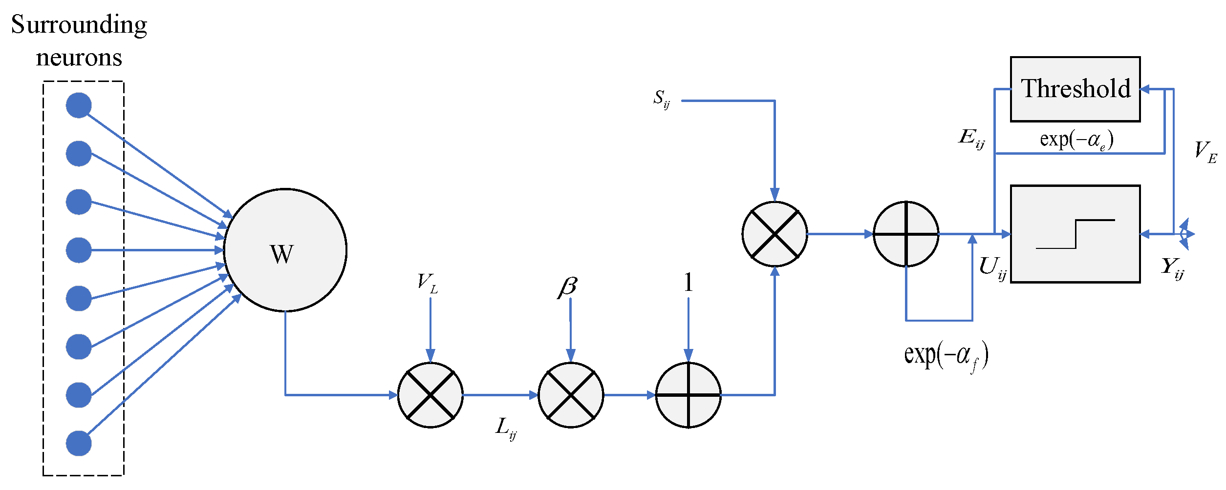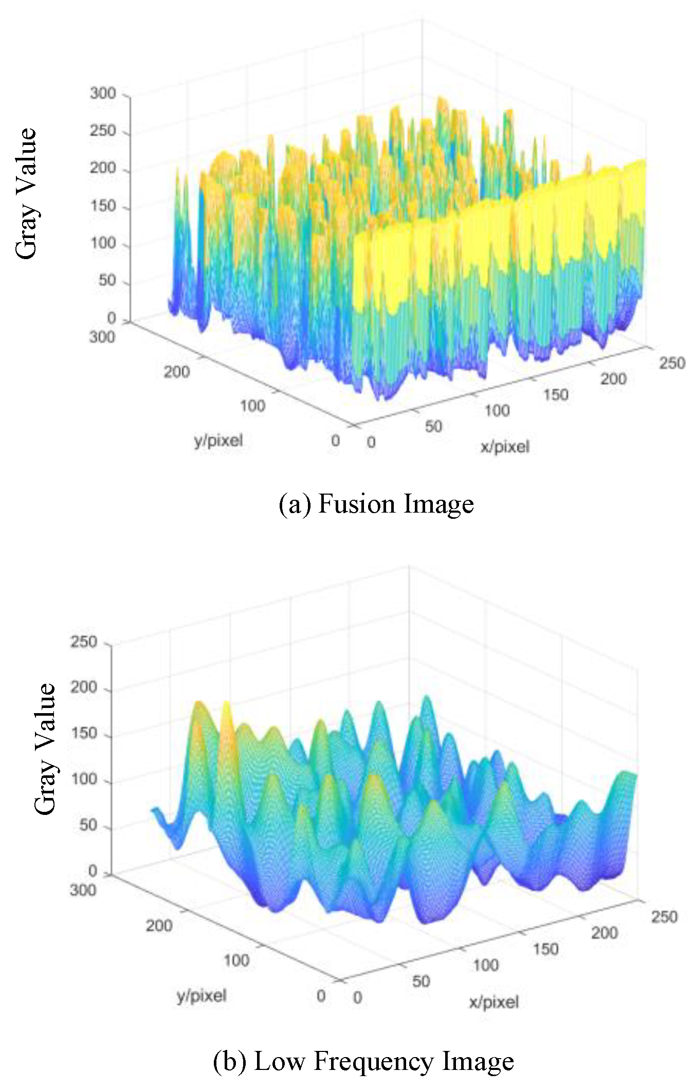In most cases, the parameters of PCNNs are empirically or manually entered, which largely limits the performance of the algorithm [18], and parametric adaptive PCNN (PAPCNN) [19] is introduced into the field of foam image fusion to overcome the difficulty of setting free parameters. For low-frequency fusion, this paper proposes a new low-frequency fusion strategy based on image quality detection, which obtains the fusion weights of low frequency by detecting the image quality of low-frequency sub-bands and adjusts the fusion weight according to the different image quality of different low-frequency sub-bands, which not only retains the background information contained in low frequency but also retains a small amount of detailed information.

There is a strong correlation between foam features and flotation conditions, and a condition recognition model can be established through various features of foam images. Liu et al. [20] proposed to introduce a gray correlation matrix to extract foam textures and to use a self-organizing neural network to identify the foam condition; Patel et al. [21] proposed a support vector machine regression (SVR) based algorithm that can better predict the quality of iron ore images. Guyon [22] proposed an SVM-RFE model, which eliminates features one by one in a recursive manner to reduce the data dimensionality. From the above references, it can be seen that there are large errors, redundant information, and poor relations in some features. Deep learning solves the above problems. Additionally, dynamic data distribution [4,23], disease detection [24], and image recognition [25] are typical applications of CNN and deep learning. Convolutional neural networks can extract effective features from images and perform deep learning to avoid complex feature extraction. The steps are convolution, pooling and other operations [25], extraction of features with discriminatory, feeding into classifiers for target recognition for training, and using the trained classifiers to complete the operation of identity recognition considering unknown targets [26,27].

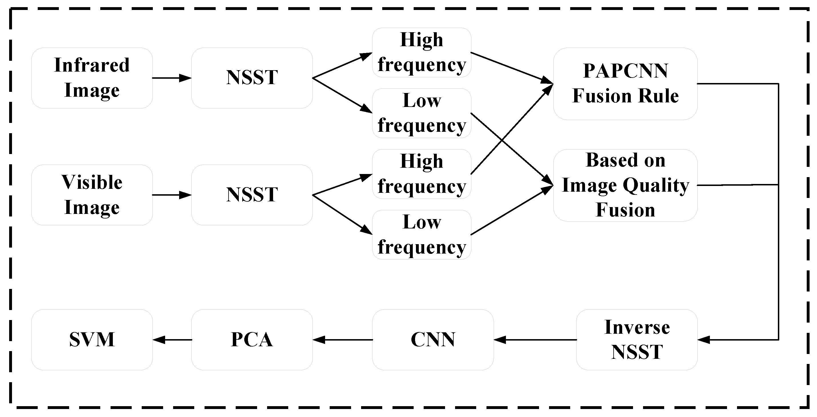
Based on the above research, this paper proposes a mineral foam flotation classification model based on multi-modality image fusion in visible and infrared gray. Firstly, the source image is scale decomposed using NSST. Secondly, the fusion of high-frequency sub-bands uses PAPCNN, and the fusion of low-frequency sub-bands is based on an image quality detection fusion method. Thirdly, NSST inversion reconstructs the new fused image. Finally, the image features are extracted using CNN, and after dimensionality reduction by PCA, the mineral foam images are classified using SVM.

2. Methods

2.1. Foam Image Fusion

After fusing the mineral foam images, the images can be divided into three categories, as shown in Figure 1., according to characteristics of foam working conditions. The characteristics are: (a) overflow foam, with a reflective surface and rough texture, indicating that the phenomenon is caused by excessive addition of flotation reagent; (b) normal foam, with suitable flotation reagent, mineral concentration and grinding fineness, flotation foam size, uniform distribution, well-defined, and the best flotation performance; (c) sinking foam, the liquid level drops, the foam cannot be scraped out, most of them are small foams, and the foam collapses seriously due to insufficient grinding fineness, a sudden increase in processing volume, or insufficient concentration of flotation reagent. Therefore, only (b) is qualified foam, and (a) and (c) are unqualified foams. When category (a) foam occurs, the amount of flotation reagent can be reduced appropriately or the amount of mineral can be increased. When category (c) foam occurs, the amount of flotation reagent or the fineness of minerals should be increased.

2.1.1. Non-Subsampled Shearlet Transform (NSST)

Compared with early MST methods such as the pyramid and wavelet, the Shearlet can capture the detailed features of an image more effectively. The Shearlet transform process is similar to the Contourlet transform process, but the directional filter in Contourlet becomes the Shearlet filter. In addition, the inverse Shearlet transform process only requires summing the Shearlet filter instead of inverse directional filter banks as in Contourlet [19].

Despite the many advantages of the Shearlet, the Shearlet lacks translation invariance, which is a critical feature for image fusion to prevent the Gibbs phenomenon due to the lack of translation invariance. To overcome this drawback, Gao [16] et al. proposed NSST, which does not use the downsampling process in the process of the Shearlet transform. NSST includes non-downsampling multi-scale decomposition by non-subsampled pyramid filters (NSPFs) and directional localization by Shift Invariant Shearlet (SFBs) [28], which has multi-scale, multi-direction, and shift invariance, and avoids Gibbs phenomenon.

The NSST first decomposes the source image by K-layer NSPF to obtain the sub-band images with the same size as the source image, including K high-frequency sub-bands and 1 low-frequency sub-bands. After multi-scale decomposition, the high-frequency sub-bands are decomposed with SFB for direction localization to obtain high-frequency coefficients in different directions. Figure 2 shows a three-stage flow chart of NSST decomposition.

2.1.2. Parameter Adaptive Pulse Coupled Neural Network (PAPCNN)

PCNN is the earliest neural-network model based on the cat vision principle, which has global coupling and pulse synchronization. PCNN is based on iterative computation and can extract effective information directly without learning and training. The application of PCNN in image processing is usually a single-layer network with two-dimensional array input. There is a one-to-one correspondence between the input image pixels and PCNN neurons, so the number of neurons is equal to the number of pixels. Each neuron relates to adjacent neurons for information transmission and coupling. There are five parameters in the PCNN model that need to be set by yourself, including the attenuation coefficient, the link strength, and so on [29]. The PAPCNN model is shown in Formula (1):

$$\begin{array}{l}{F}_{ij}[n]=S_{ij}\\ L_{ij}[n]=V_L{\displaystyle \sum _{kl}{W}_{ijkl}{Y}_{kl}[n-1]}\\ U_{ij}[n]=e^{-{\alpha }_f}{U}_{ij}[n-1]+F_{ij}[n](1+\beta L_{ij}[n])\\ Y_{ij}[n]=\{\begin{array}{l}1, if U_{ij}[n]>E_{ij}[n-1]\\ 0, otherwise\end{array}\\ E_{ij}[n]=e^{-{\alpha }_e}{E}_{ij}[n-1]+V_E{Y}_{ij}[n]\end{array}$$

(1)

$F_{ij}[n]$ and $L_{ij}[n]$ are the two main inputs of positional neurons at position $(i,j)$ in iteration n: feedback input and connection input. In the whole iterative process, $F_{ij}[n]$ is the intensity of the input image $S_{ij}$, and $L_{ij}[n]$ is associated with the firing state of the eight adjacent neurons in the previous iteration through the synaptic weight $W_{ijkl}$.

$$W_{ijkl}=\left[\begin{array}{ccc}0.5& 1& 0.5\\ 1& 0& 1\\ 0.5& 1& 0.5\end{array}\right]$$

(2)

$U_{ij}[n]$ is the internal activity, and when it is compared with the dynamic threshold $E_{ij}[n-1]$ of the previous iteration, the neuron $N_{ij}$ is judged whether to start ($Y_{ij}[n]=1$) or not to start ($Y_{ij}[n]=0$). If the neuron $N_{ij}$ fires successfully once, the dynamic threshold $E_{ij}[n]$ will increase with amplitude $V_E$. If the neuron $N_{ij}$ fails to fire, the dynamic threshold will decay with $e^{-{\alpha }_e}$ coefficient. The parameters $V_L$ and $V_E$ denote the amplitudes of the connection input L and the dynamic threshold E, and the parameters ${\alpha }_f$ and ${\alpha }_e$ denote L and E [30]. $Y_{ij}[n]=0,U_{ij}[n]=0,E_{ij}[n]=0$ when this model is initialized. Therefore, all neurons with non-zero intensity fire in the first iteration. There are five self-set parameters in the PAPCNN model: ${\alpha }_f$, ${\alpha }_e$, $V_L$, $V_E$ and $\beta$, as shown in Formula (3).

$$\begin{array}{l}{\alpha }_f=\log (1/\sigma (S))\\ {\alpha }_e=\ln (\frac{\frac{V_E}{S^{\prime }}}{\frac{1-e^{-3{\alpha }_f}}{1-e^{-{\alpha }_f}}+6\beta V_L{e}^{-{\alpha }_f}})\\ V_L=1\\ V_E=e^{-{\alpha }_f}+1+6\beta V_L\\ \beta =\frac{(S_{\max }/S^{\prime })-1}{6}\end{array}$$

(3)

where $\sigma (S)$ denotes the standard deviation of input image S, $S^{\prime }$ and $S_{\max }$ denote the normalized Otsu threshold and the maximum intensity of the input image. The architecture of the PAPCNN model is shown in Figure 3.

The absolute value of the high-frequency sub-band is taken as the network input, that is, the feedback input is $F_{ij}[n]=\left|H_S^{l,k}\right|,S\in \{I,V\}$,$I,V$, which respectively represent the infrared foam image and the visible foam image, and the activity of the high-frequency coefficient is measured by the total number of firing in the entire iterative process. The number of firings is accumulated by adding the following steps at the end of each iteration:

$$T_{ij}[n]=T_{ij}[n-1]+Y_{ij}[n]$$

(4)

Therefore, the number of firings for each neuron is $T_{ij}[N]$, and N is the total number of iterations. For the corresponding high-frequency sub-bands $H_I^{l,k}$ and $H_V^{l,k}$, their PAPCNN firing times can be calculated using $T_{I,ij}^{l,k}[N]$ and $T_{V,ij}^{l,k}[N]$, respectively. The high-frequency fusion rule is shown in Formula (5):

$$H_F^{l,k}(i,j)=\{\begin{array}{l}{H}_V^{l,k}(i,j), if T_{V,ij}^{l,k}[N]\ge T_{I,ij}^{l,k}[N]\\ H_I^{l,k}(i,j), otherwise\end{array}$$

(5)

This indicates that the coefficient with the larger firing number will be selected as the fusion coefficient.

2.1.3. Fusion Rules Based on Image Quality Detection

The low-frequency sub-bands represent the mostly smooth regions of the image, which contain most of the image energy and typically represent the background. The pixel-intensity distribution of the image is also mainly reflected in the low-frequency information. The traditional simple average low-frequency fusion method will cause the loss of image energy and detail loss of the fused image, and the fused image will reduce the contrast, which is not in accordance with human visual perception [12]. According to the above problems, a new low-frequency fusion rule based on image quality detection is proposed to evaluate and quantify image information quality, spatial gradient, and other image quality evaluations of visible and infrared low-frequency sub-band images. The low-frequency fusion weights are determined by the image quality, and weights will be adjusted according to different low-frequency sub-bands with high flexibility, maintaining the high-contrast features of the fused image. The fusion image preserves the background information and energy information contained in the low-frequency, which facilitates subsequent observation and processing.

Image quality detection evaluates the quality of low-frequency images. The following evaluation coefficients are selected to evaluate low-frequency images, and the weights are assigned and fused to the low-frequency images according to the evaluation results.

1, Entropy EN, the mathematical formula for measuring the amount of information contained in a low-frequency image is defined as follows:

$$EN=-{\displaystyle \sum _{l=0}^{L-1}{p}_l {\log }_2 p_l}$$

(6)

L is the number of gray levels and $p_l$ is the normalized histogram of the corresponding gray levels in the low-frequency image. The larger the EN, the more information is contained in the low-frequency image, but if there is more noise in the image, the EN value will also be high. Therefore, EN is used as an auxiliary measure.

2, Standard Deviation SD, reflects the distribution and contrast of low-frequency images, and the mathematical formula is defined as follows:

$$SD=\sqrt{{\displaystyle {\sum }_{i=1}^M{\displaystyle {\sum }_{j=1}^N{(L(i,j)-\mu )}^2}}}$$

(7)

$\mu$ is the average value of low-frequency images. High-contrast images can produce larger SD. The human visual system is more sensitive to high-contrast images. The larger the SD, the better the visual effect of low-frequency images.

3, Spatial Frequency SF, is a gradient-based image quality standard, which is divided into a horizontal gradient and a vertical gradient, also known as the spatial row frequency RF and the column frequency CF. The SF metric can effectively measure the gradient distribution of the image and reveal the details and texture of the image. The mathematical formula is defined as follows:

$$\begin{array}{l}SF=\sqrt{R{F}^2+C{F}^2}\\ RF=\sqrt{{\displaystyle {\sum }_{i=1}^M{\displaystyle {\sum }_{j=1}^N{(L(i,j)-L(i,j-1))}^2}}}\\ CF=\sqrt{{\displaystyle {\sum }_{i=1}^M{\displaystyle {\sum }_{j=1}^N{(L(i,j)-L(i-1,j))}^2}}}\end{array}$$

(8)

The higher SF value means that the low-frequency image contains rich edge information and texture information.

4, Average Gradient AG, the gradient information of a low-frequency image is quantized, and the formula is defined as follows:

$$AG=\frac{1}{MN}{\displaystyle \sum _{i=1}^M{\displaystyle \sum _{j=1}^N\sqrt{\frac{\nabla F_x^2(i,j)+\nabla F_y^2(i,j)}{2}}}}$$

(9)

where $\nabla F_x(i,j)=L(i,j)-L(i+1,j)$, $\nabla F_y(i,j)=L(i,j)-L(i,j+1)$. The higher the AG value is, the more gradient information is contained in the low-frequency image. The formula for a low-frequency image fusion is as follows:

$$\begin{array}{l}{L}_F={\omega }_1{L}_I+{\omega }_2{L}_V\\ {\omega }_1{}^{\prime }=E{N}_I+S{D}_I+S{F}_I+A{G}_I\\ {\omega }_2{}^{\prime }=E{N}_V+S{D}_V+S{F}_V+A{G}_V\\ {\omega }_1=\frac{{\omega }_1{}^{\prime }}{{\omega }_1{}^{\prime }+{\omega }_2{}^{\prime }},{\omega }_2=\frac{{\omega }_2{}^{\prime }}{{\omega }_1{}^{\prime }+{\omega }_2{}^{\prime }}\end{array}$$

(10)

It shows that the higher the weight of the low-frequency image after fusion, the higher the low-frequency image with high image quality. Comparison of the low-frequency image and the fused image as shown in Figure 4.

Then, the fused image F is obtained by performing the inverse NSST on $\{H_F^{l,k}(i,j),L_F\}$. The image fusion flow chart is shown in Figure 5. The low-frequency fusion method proposed in this paper performs a quality assessment on the low-frequency image to determine the fusion weight of the low-frequency image. The fused low-frequency image not only retains the detailed background information but also highlights the foam target. So, the fused foam image not only contains rich texture details but also highlights the foam target. It is beneficial to feature extraction and working condition classification of foam flotation.

2.2. Image Classification Based on CNN-PCA-SVM

A complete CNN consists of an input layer, convolution layers, pooling layers, full connection layers, and an output layer. The input layer is mainly used for image data reception. The image data is directly transferred to subsequent hidden layers for forward propagation and error back-propagation training. The convolution layer is mainly used for feature extraction of input image data, which will output a feature map of input image data and transfer it to the next hidden layer. The pooling layer is usually used to solve the case of excessive computation and low-computational efficiency of the feature maps. The fully connected layer converts the pooled feature graph into a one-dimensional vector [31].

PCA is one of the most widely used data dimensionality reduction algorithms. The main idea of PCA is to map n-dimensional features to k-dimensional. By calculating the covariance matrix of the data, the eigenvalues and eigenvectors of the covariance matrix are obtained, and the matrix consisting of eigenvectors corresponding to k features with the largest eigenvalue is selected, thus realizing the dimensionality reduction of feature data [32].

SVM is a statistical-based machine learning method [33] for non-linear separable problems, where the non-linear problem is transformed into a linear separable problem in a high-dimensional space. The approach used is to introduce a kernel function $K(x_i,x_j)$, which must satisfy the Mercer condition, and the Mercer kernel approximately corresponds to a nonlinear mapping $\psi :R^n\to H$ from the input space to the high-dimensional Hilbert space.

$$K(x_i,x_j)=(\psi (x_i)·\psi (x_j))$$

(11)

Nonlinear mathematical formula of SVM:

$$\begin{array}{c}W(\alpha )={\displaystyle \sum _{i=1}^n{\alpha }_i}-\frac{1}{2}{\displaystyle \sum _{i,j=1}^n{\alpha }_i}{\alpha }_j{y}_i{y}_j(\psi (x_i)·\psi (x_j))\\ ={\displaystyle \sum _{i=1}^n{\alpha }_i}-\frac{1}{2}{\displaystyle \sum _{i,j=1}^n{\alpha }_i}{\alpha }_j{y}_i{y}_{j}K(x_i,x_j)\end{array}$$

(12)

The classification function is:

$$\begin{array}{cc}\hfill f(x)& =\mathrm{sgn}({\displaystyle \sum _{i=1}^n{\alpha }^{\ast }{}_i}{y}_i\psi (x_i)·\psi (x)+b^{\ast })\hfill \\ & =\mathrm{sgn}({\displaystyle \sum _{i=1}^n{\alpha }^{\ast }{}_i}{y}_{i}K(x_i,x)+b^{\ast })\hfill \end{array}$$

(13)

In this paper, CNN is used to extract the feature vectors of flotation froth images using a VGG16 network [34] and a Sigmoid activation function. Although a large amount of sample data provides rich information for training, it also increases redundant information, so PCA is used to reduce the feature dimension and extract the key features of the image, which can greatly preserve the data features while reducing the correlation between adjacent pixels of the image. The SoftMax classifier in CNN can only make the output data of the fully connected layer conform to the probability distribution, which cannot improve the classification effect, so the SoftMax classifier of CNN is changed to SVM for classification, and the reduced-dimensional data is used as the input of SVM for image classification. The CNN model for feature extraction is shown in Figure 6. The structure of the CNN-PCA-SVM model is shown in Figure 7. Due to the limitation of the number of datasets, training CNN from scratch does not achieve the desired effect. Using transfer learning can solve this issue [35]. VGG16 is adopted as our starting point, which is pre-trained on ImageNet.

3. Results

3.1. Algorithm Flow

The whole algorithm schematic is shown in Figure 8.

This algorithm is mainly divided into six main parts. The specific steps are as follows: 1. multi-scale decomposition of infrared and visible gray foam images using NSST; 2. low-frequency fusion algorithm based on image quality method for low-frequency sub-band images of infrared gray and visible gray images, and PAPCNN fusion algorithm for high-frequency; 3. inverse NSST fusion of fused high and low-frequency sub-band images; 4. fuse images using CNN for feature extraction; 5. reduce the dimension of the feature matrix using PCA; 6. classify the condition of the reduced feature matrix using SVM.

3.2. Experimental Data

All the experiments in this paper were run on Windows10, MATLAB2022a, python3.9, TensorFlow 2.10.0. The dataset of this paper is collected from Guangxi China Tin Group Co., Ltd. (Liuzhou, China) and is characterized by comprehensiveness, richness, and authenticity. The experiment is divided into two parts, the first part is image fusion, and the second part is image classification. There are 3900 visible and infrared gray images respectively, and a total of 3900 images are fused. All source images were scaled to the same spatial resolution of 224 × 224 pixels. To avoid complexity, the scale of foam images was adjusted from 0-255 to 0-1.

3.2.1. Image Fusion

The parameters of the image fusion algorithm are set. Two main parameters are set: (1) the number of NSST decomposition sub-band levels, and (2) the number of iterations of PAPCNN.

(1) The level K of NSST decomposition sub-band levels is from 1 to 4 respectively, and the direction number of each decomposition level is determined. The direction number generally decreases from fine scale to coarse scale. In this paper, the number of directions is set to 16, 16, 8, and 8 from fine to coarse. The number of directions of each level corresponding to different decomposition sub-band stages is shown in

Table 1. The number of NSST decomposition sub-band levels and the direction number of each level.

Number of Decomposition Sub-Bands	The Direction Number of Each Level
1	16
2	16, 16
3	16, 16, 8
4	16, 16, 8, 8

.

In this experiment, the fusion image is evaluated based on Peak Signal to Noise Ratio (PSNR), Mutual Information (MI), Average Gradient (AG), Mean Square Error (MSE), Standard Deviation (SD), and Visual Quality Fidelity (VIF) [7]. PSNR is the ratio of peak power to noise power in the fused image, which reflects the distortion in the fusion process. The larger the value is, the closer the fused image is to the source image, and the less distortion is produced by the fusion method. MI is a quality index that measures the amount of information transferred from the source image to the fused image. A larger value indicates that more information is transferred from the source image to the fused image, indicating a good fusion performance. AG quantifies the gradient information of the fused image to represent its details and textures. The larger the value, the more gradient information the fused image contains and the better the performance of the fusion algorithm. MSE indicates the error between the fused image and the source images. The smaller the value, the better the fusion performance, which means that the fused image is closer to the source image and the error in the fusion process is smaller. SD is based on the statistical concept that reflects the distribution and contrast of the fused image. The higher the contrast of the fused image, the higher the SD value, which means that the fused image achieves good visuals. VIF measures the information fidelity of the fused image, which is consistent with the human visual system. By measuring the fidelity of visual information between the fused image and each source image, the higher the value, the better the performance.

Figure 9 shows the effect of parameter K on the fused image indices, and the number of iterations N of PAPCNN is fixed at 110. In the case of N = 4, most of the indices of the sample data are the best except for the MI index which gradually decreases. From the above information, it can be seen that when K = 4, most of the indices of image fusion are better and the effect of image fusion is better.

(2) Number of PAPCNN iterations, is set to 70, 90, 110, 130, and 150. The results are shown in Figure 10, where fixed K = 4. As shown in Figure 10, the sample foam images have the best performance, where data 1 has the best performance except MI at N = 110, data 2 has the best performance except PSNR at N = 110, and data 3 has the best performance at N = 110 except MI. Therefore, combining Figure 9 and Figure 10, we can get the best effect of image fusion when K = 4 and N = 110.

The image fusion method in this paper is compared with the method of [18], the method of [36], and the maximum fusion method. The fused image indexes are shown in Figure 11. For the PSNR, the fusion method in this paper is the best. For most of the samples, the MI index is the best. In this paper, the MSE index and the error are smaller, the fusion performance is better, and the fusion method obtains the smallest index value. The SD and VIF indices, this method is significantly better than other fusion methods. In summary, it can be concluded that the performance index of the method in this paper is better than the method of [18], the method of [36], and the maximum fusion method. The fusion method proposed in this paper has less distortion, more gradient information, less fusion error, and high contrast implying a good visual effect.

3.2.2. Image Classification

By adding noise, rotation and translation to the image, the data were expanded to 4500 foam images of pixel size 224 × 224 × 3 (1500 images per type). The noisy images were added to improve the robustness of the model. Since the original images were gray images, these images were uniformly converted into RGB images for feature extraction by convolution neural network.

Three hundred foam images of each type were separated separately to form a blind dataset (not known to a trained model with previous tool configurations) [37]. The training dataset and testing dataset are divided into 80%/20%. They were constructed with 960 foam images and 240 foam images, respectively, under three different conditions. Meanwhile, the model was trained using a 10-fold cross-validation approach [23].

For the structure of the neural network, we chose the VGG16 model. Because the data sample is small and transferring learning, we fine-tuned the CNN parameters that had already been trained on ImageNet. The learning rate of the proposed model was 0.0001. Epoch was set to 100, batch size was set to 32, dropout was set to 0.5 and the activation function used the ReLu function.

After extracting 1000 features using the CNN, standardization has been performed on the data [24]. Three hundred eigenvalues were selected as shown in Figure 12. In the SVM model, the two parameters with the RBF kernel have the greatest influence on the accuracy: penalty parameter ($c$) and gamma ($\gamma$). We referred to the data in [4] and finally chose $c=10,\gamma =0.01$.

As shown in Figure 13, the confusion matrix of the 10-fold cross-validation mode is demonstrated. The classification accuracy is 93.7%.

Table 2. Performance indicators of classification considering 10-fold cross-validation mode.

Type	Precision	Recall	F1	Accuracy (%)
Overflow	0.97	0.88	0.92	-
Normal	0.91	0.95	0.93	-
Sinking	0.94	0.98	0.96	-
Average	0.94	0.94	0.94	93.7

shows performance indicators of classification considering a 10-fold cross-validation mode. Figure 14 shows the confusion matrix of the training dataset. The classification accuracy is 95.9%.

Table 3. Performance indicators of classification considering training dataset.

Type	Precision	Recall	F1	Accuracy (%)
Overflow	0.98	0.93	0.95	-
Normal	0.94	0.97	0.95	-
Sinking	0.96	0.98	0.97	-
Average	0.96	0.96	0.96	95.9

shows performance indicators of classification considering the training dataset. Figure 15 shows the confusion matrix of the testing dataset. The classification accuracy is 94.2%.

Table 4. Performance indicators of classification considering testing dataset.

Type	Precision	Recall	F1	Accuracy (%)
Overflow	0.97	0.88	0.92	-
Normal	0.90	0.96	0.93	-
Sinking	0.96	0.98	0.97	-
Average	0.94	0.94	0.94	94.2

shows performance indicators of classification considering the testing dataset.

The confusion matrix of the CNN-PCA-SVM model considering the blind dataset is shown in Figure 16.

Table 5. Performance indicators of classification considering the testing dataset.

Type	Precision	Recall	F1	Accuracy (%)
Overflow	0.92	0.90	0.91	-
Normal	0.90	0.92	0.91	-
Sinking	0.96	0.95	0.95	-
Average	0.93	0.92	0.92	92.3

shows performance indicators of classification considering the blind dataset.

Processing time for classification as shown in

Table 6. Processing time for classification.

Type	Running Time (sec)
10-fold cross-validation mode	7064
Training dataset	3405
Testing dataset	203
Blind dataset	216

. From the above graphs, it can be learned that the average accuracy of CNN-PCA-SVM reaches 92.3%, with high average classification accuracy and efficiency. The VGG16-PCA-SVM model surpassed the existing models adopted in other literature, as shown in

Table 7. Accuracy comparison of different models with existing models.

Model	Accuracy (%)
[38]	85.5
[39]	90.3
[40]	91.6
[4]	89.3
This model	92.3

. The experimental results show that the CNN-PCA-SVM model performs better in the small dataset of foam images and the model for foam flotation classification, which meets the industrial requirements. The running time for classification prediction of a foam image is 0.24 s.

4. Conclusions and Future Directions

In this paper, a new foam image fusion method is proposed. The fused mineral foam image contains rich texture detail features and highlights the mineral foam outline, which is beneficial to mineral foam flotation feature extraction and conditions classification.

The CNN-PCA-SVM model based on Multi-modal foam image fusion was successfully proposed, which can classify three foam conditions. After effective design, training, testing, and verification, the classification accuracy is 92.3% considering the blind dataset.

This shows that the image fusion model proposed in this paper is suitable for feature extraction of mineral foam images, which can be used for cross-domain image fusion. The classification model is applicable to the classification of mineral foam quality, and this trained classification model can be used for cross-domain data distribution.

The future work will feed the model with a large amount of data to reduce misclassification, increase the robustness of the model in a highly noisy environment through model augmentation [41], and build a real-time detection error classification system.

References

1. Gui, W.; Yang, C.; Xu, D.-G.; Lu, M.; Xie, Y. Machine-vision-based Online Measuring and Controlling Technologies for Mineral Flotation—A Review. Acta Autom. Sin. 2013, 39, 1879–1888. [Google Scholar] [CrossRef]
2. Moolman, D.W.; Aldrich, C.; Van Deventer, J.S.J.; Stange, W.W. Digital image processing as a tool for on-line monitoring of froth in flotation plants. Miner. Eng. 1994, 7, 1149–1164. [Google Scholar] [CrossRef]
3. Lu, M.; Gui, W.H.; Peng, T.; Xie, Y.F. Equivalent size distribution feature extraction of flotation froth image. Control. Decis. 2015, 30, 131–136. [Google Scholar]
4. Li, Z.; Gui, W.; Zhu, J. Fault detection in flotation processes based on deep learning and support vector machine. J. Cent. South Univ. 2019, 26, 2504–2515.1. [Google Scholar] [CrossRef]
5. Morar, S.H.; Bradshaw, D.J.; Harris, M.C. The use of the froth surface lamellae burst rate as a flotation froth stability measurement. Miner. Eng. 2012, 36, 152–159. [Google Scholar] [CrossRef]
6. Zhang, J.; Liao, Y.; Chen, S.; Wang, W. Floatation Dosing State Recognition Based on Multiscale CNN Features and RAE-KELM. Laser Optoelectron. Prog. 2021, 58, 417–426. [Google Scholar]
7. Ma, J.; Ma, Y.; Li, C. Infrared and visible image fusion methods and applications: A survey. Inf. Fusion 2019, 45, 153–178. [Google Scholar] [CrossRef]
8. Fernandez-Beltran, R.; Haut, J.M.; Paoletti, M.E.; Plaza, J.; Plaza, A.; Pla, F. Remote Sensing Image Fusion Using Hierarchical Multimodal Probabilistic Latent Semantic Analysis. IEEE J. Sel. Top. Appl. Earth Obs. Remote Sens. 2019, 11, 4982–4993. [Google Scholar] [CrossRef]
9. Singh, R.; Vatsa, M.; Noore, A. Integrated multilevel image fusion and match score fusion of visible and infrared face images for robust face recognition. Pattern Recognit. 2008, 41, 880–893. [Google Scholar] [CrossRef] [Green Version]
10. Liu, Y.; Chen, X.; Wang, Z.; Wang, Z.J.; Ward, R.K.; Wang, X. Deep learning for pixel-level image fusion: Recent advances and future prospects. Inf. Fusion 2018, 42, 158–173. [Google Scholar] [CrossRef]
11. Kumar, P.; Mittal, A.; Kumar, P. Fusion of Thermal Infrared and Visible Spectrum Video for Robust Surveillance; Springer: Berlin/Heidelberg, Germany, 2006; pp. 528–539. [Google Scholar]
12. Liu, Y.; Liu, S.; Wang, Z. A general framework for image fusion based on multi-scale transform and sparse representation. Inf. Fusion 2015, 24, 147–164. [Google Scholar] [CrossRef]
13. Li, H.; Manjunath, B.; Mitra, S. Multisensor Image Fusion Using the Wavelet Transform. Graph. Model. Image Process. 1995, 57, 235–245. [Google Scholar] [CrossRef]
14. Do, M.N.; Vetterli, M. The contourlet transform: An efficient directional multiresolution image representation. IEEE Trans. Image Process. A Publ. IEEE Signal Process. Soc. 2005, 14, 2091–2106. [Google Scholar] [CrossRef] [Green Version]
15. Zhang, Q.; Guo, B. Multifocus image fusion using the nonsubsampled contourlet transform. Signal Process. 2009, 89, 1334–1346. [Google Scholar] [CrossRef]
16. Gao, G.; Xu, L.; Feng, D. Multi-focus image fusion based on non-subsampled shearlet transform. IET Image Process. 2013, 7, 633–639. [Google Scholar]
17. Eckhorn, R.; Reitboeck, H.J.; Arndt, M.T.; Dicke, P. Feature Linking via Synchronization among Distributed Assemblies: Simulations of Results from Cat Visual Cortex. Neural Comput. 2014, 2, 293–307. [Google Scholar] [CrossRef]
18. Yin, M.; Liu, X.; Liu, Y.; Chen, X. Medical Image Fusion With Parameter-Adaptive Pulse Coupled Neural Network in Nonsubsampled Shearlet Transform Domain. IEEE Trans. Instrum. Meas. 2019, 68, 49–64. [Google Scholar] [CrossRef]
19. Chen, Y.; Park, S.K.; Ma, Y.; Ala, R. A new automatic parameter setting method of a simplified PCNN for image segmentation. IEEE Trans. Neural Netw. 2011, 22, 880–892. [Google Scholar] [CrossRef]
20. Liu, W.; Lu, M.; Wang, F.; Wang, Y. Extraction of Textural Feature and Recognition of Coal Flotation Forth. CIESC J. 2003, 830–835. Available online: https://kns.cnki.net/kcms2/article/abstract?v=3uoqIhG8C44YLTlOAiTRKgchrJ08w1e7ZCYsl4RS_3i2FXAmiHbArp5T3rBRxOFO-FKDw_byrUbXt_3qgLxiKUMvj38ZwLPQ&uniplatform=NZKPT (accessed on 5 March 2023).
21. Patel, A.K.; Chatterjee, S.; Gorai, A.K. Development of a machine vision system using the support vector machine regression (SVR) algorithm for the online prediction of iron ore grades. Earth Sci. Inform. 2019, 12, 197–210. [Google Scholar] [CrossRef]
22. Guyon, I.; Weston, J.; Barnhill, S.; Vapnik, V. Gene Selection for Cancer Classification using Support Vector Machines. Mach. Learn. 2002, 46, 389–422. [Google Scholar] [CrossRef]
23. Kale, A.P.; Wahul, R.M.; Patange, A.D.; Soman, R.; Ostachowicz, W. Development of Deep Belief Network for Tool Faults Recognition. Sensors 2023, 23, 1872. [Google Scholar] [CrossRef]
24. Nahiduzzaman, M.; Goni, M.O.F.; Anower, M.S.; Islam, M.R.; Ahsan, M.; Haider, J.; Gurusamy, S.; Hassan, R.; Islam, M.R. A Novel Method for Multivariant Pneumonia Classification Based on Hybrid CNN-PCA Based Feature Extraction Using Extreme Learning Machine with CXR Images. IEEE Access 2021, 9, 147512–147526. [Google Scholar] [CrossRef]
25. Simonyan, K.; Zisserman, A. Very Deep Convolutional Networks for Large-Scale Image Recognition. Comput. Sci. 2014. Available online: https://arxiv.org/abs/1409.1556 (accessed on 5 March 2023).
26. Shafiq, M.; Gu, Z. Deep Residual Learning for Image Recognition: A Survey. Appl. Sci. 2022, 12, 8972. [Google Scholar] [CrossRef]
27. Wagner, S.A. SAR ATR by a combination of convolutional neural network and support vector machines. IEEE Trans. Aerosp. Electron. Syst. 2016, 52, 2861–2872. [Google Scholar] [CrossRef]
28. Easley, G.; Labate, D.; Lim, W.Q. Sparse directional image representations using the discrete shearlet transform. Appl. Comput. Harmon. Anal. 2007, 25, 25–46. [Google Scholar] [CrossRef] [Green Version]
29. Pacifici, F.; Del Frate, F. Automatic Change Detection in Very High Resolution Images with Pulse-Coupled Neural Networks. IEEE Geosci. Remote Sens. Lett. 2010, 7, 58–62. [Google Scholar] [CrossRef] [Green Version]
30. Wang, Z.; Ma, Y.; Cheng, F.; Yang, L. Review of pulse-coupled neural networks. Image Vis. Comput. 2009, 28, 5–13. [Google Scholar] [CrossRef]
31. Guan, S.; Zhang, Y.; Tian, Z. Research on Human Behavior Recognition based on Deep Neural Network. In Proceedings of the 3rd International Conference on Mechatronics Engineering and Information Technology(ICMEIT 2019), Dalian, China, 29–30 March 2019; pp. 793–797, Analysis and Extension of the PCA Method. [Google Scholar]
32. Catanzaro, B.; Sundaram, N.; Keutzer, K. Fast support vector machine training and classification on graphics processors. In Proceedings of the 25th International Conference on Machine Learning, Helsinki, Finland, 5–9 July 2008; pp. 104–111. [Google Scholar]
33. Kramar, V.A.; Alchakov, V.V.; Dushko, V.R.; Kramar, T.V. Application of support vector machine for prediction and classification. J. Phys. Conf. Ser. 2018, 1015, 032070. [Google Scholar] [CrossRef]
34. Jiang, X.; Liu, J.; Wang, L.; Lei, B.; Hu, M. Flotation condition recognition based on multi-scale convolutional neural network and LBP algorithm. J. Min. Sci. Technol. 2023, 8, 202–212. [Google Scholar]
35. Ng, H.W.; Nguyen, V.D.; Vonikakis, V.; Winkler, S. Deep Learning for Emotion Recognition on Small Datasets Using Transfer Learning. In Proceedings of the 2015 ACM on International Conference on Multimodal Interaction, Seattle, WA, USA; pp. 443–449. Available online: https://dl.acm.org/doi/10.1145/2818346.2830593 (accessed on 5 March 2023).
36. Chen, J.; Li, X.; Luo, L.; Mei, X.; Ma, J. Infrared and visible image fusion based on target-enhanced multiscale transform decomposition. Inf. Sci. 2020, 508, 64–78. [Google Scholar] [CrossRef]
37. Bajaj Naman, S.; Patange Abhishek, D.; Jegadeeshwaran, R.; Pardeshi Sujit, S.; Kulkarni Kaushal, A.; Ghatpande Rohan, S. Application of metaheuristic optimization based support vector machine for milling cutter health monitoring. Intell. Syst. Appl. 2023, 18. Available online: https://www.sciencedirect.com/science/article/pii/S2667305323000212 (accessed on 5 March 2023).
38. Fu, Y.; Aldrich, C. Froth image analysis by use of transfer learning and convolutional neural networks. Miner. Eng. 2018, 115, 68–78. [Google Scholar] [CrossRef]
39. Wang, X.; Chen, S.; Yang, C.; Xie, Y. Process working condition recognition based on the fusion of morphological and pixel set features of froth for froth flotation. Miner. Eng. 2018, 128, 17–26. [Google Scholar] [CrossRef]
40. Fu, Y.; Aldrich, C. Flotation froth image recognition with convolutional neural networks. Miner. Eng. 2019, 132, 183–190. [Google Scholar] [CrossRef]
41. Patange, A.D.; Pardeshi, S.S.; Jegadeeshwaran, R.; Zarkar, A.; Verma, K. Augmentation of Decision Tree Model Through Hyper-Parameters Tuning for Monitoring of Cutting Tool Faults Based on Vibration Signatures. J. Vib. Eng. Technol. 2022, 22, 781–789. [Google Scholar] [CrossRef]
Figure 1. Classification diagram of foam flotation conditions.
Applsci 13 03512 g001
Figure 2. Diagram of NSST three-level decomposition.
Applsci 13 03512 g002
Figure 3. The architecture of the PAPCNN model.
Applsci 13 03512 g003
Figure 4. Foam image 3D display diagram.
Applsci 13 03512 g004
Figure 5. Schematic of the foam image fusion method.
Applsci 13 03512 g005
Figure 6. CNN model for features extraction.
Applsci 13 03512 g006
Figure 7. Structure of CNN-PCA-SVM model.
Applsci 13 03512 g007
Figure 8. Schematic of the foam image fusion and classification.
Applsci 13 03512 g008
Figure 9. The influence of parameters K on the performance of fused image.
Applsci 13 03512 g009
Figure 10. The influence of parameters N on the performance of fused images.
Applsci 13 03512 g010
Figure 11. Image indexes of different fusion methods.
Applsci 13 03512 g011
Figure 12. Relationship between PCA dimensions and accuracy.
Applsci 13 03512 g012
Figure 13. Confusion matrix of 10-fold cross-validation mode.
Applsci 13 03512 g013
Figure 14. Confusion matrix of the training dataset.
Applsci 13 03512 g014
Figure 15. Confusion matrix of the testing dataset.
Applsci 13 03512 g015
Figure 16. VGG16-PCA-SVM confusion matrix of the blind dataset.
Applsci 13 03512 g016