E-APTDetect: Early Advanced Persistent Threat Detection in Critical Infrastructures with Dynamic Attestation

Abstract

Advanced Persistent Threats (APTs) represent a complex series of techniques directed against a particular organization, where the perpetrator is able to hide its presence for a longer period of time (e.g., months, years). Previous such attacks have demonstrated the exceptional impact that a cyber attack may have on the operation of Supervisory Control And Data Acquisition Systems (SCADA), and, more specifically, on the underlying physical process. Existing techniques for the detection of APTs focus on aggregating results originating from a collection of anomaly detection agents. However, such approaches may require an extensive time period in case the process is in a steady-state. Conversely, this paper documents E-APTDetect, an approach that uses dynamic attestation and multi-level data fusion for the early detection of APTs. The methodology leverages sensitivity analysis and Dempster-Shafer’s Theory of Evidence as its building blocks. Extensive experiments are performed on a realistic Vinyl Acetate Monomer (VAM) process model. The model contains standard chemical unit operations and typical industrial characteristics, which make it suitable for a large variety of experiments. The experimental results conducted on the VAM process demonstrate E-APTDetect’s ability to efficiently detect APTs, but also highlight key aspects related to the attacker’s advantage. The experiments also highlight that the adversary’s advantage is affected by two major factors: the number of compromised components; and, the precision of manipulation.

1. Introduction

Traditional Supervisory Control And Data Acquisition Systems (SCADA) with isolated networks hosting proprietary hardware and protocols have transitioned towards a modern architectural model. Nowadays, SCADA systems embrace modern technological advancements offering operational benefits of control, reliability, and safety, while delivering services for new applications in various directions (e.g., Smart Grids). This pervasive modernization, however, has brought upon a new wave of cyber-security threats that exploit vulnerabilities with significant impact on the physical process [1,2].

Recently, an increasing amount of research has focused on more sophisticated attack vectors that have been found in Advanced Persistent Threats (APTs). APTs represent a complex series of techniques directed against a particular organization, where the perpetrator is able to hide its presence for a longer period of time (e.g., months, years). In this scenario, the attacker may remain undetected while conducting various operations such as infecting hosts, propagating from one network to another, gathering and sending information outside the system, and changing the behavior of critical industrial components (e.g., Programmable Logical Controllers—PLCs). Examples of well-known APTs in the industrial sector include the Stuxnet malware [1], Duqu [3], and, more recently, cyber attacks against energy infrastructures [2].

In order to address the detection of APTs, various techniques have been proposed. Traditionally, firewalls, Intrusion Detection Systems, and Intrusion Prevention Systems, combined with network segmentation and the deployment of these components in several parts of the network, can provide a first level of defense [4]. However, to address unknown attacks, anomaly detection proved to bring significant advantages in detecting abnormal behavior [5,6]. In addition to these, recent techniques particularly address APTs by quantifying the output of a wide variety of anomaly detection algorithms and techniques [7,8,9,10].

While previous APT detection techniques have focused on aggregating results originating from a collection of anomaly detection agents [8,9,11] that base their decisions on system observations, we consider a more proactive approach aimed to facilitate early APT detection. Accordingly, this paper documents E-APTDetect, an approach for the early detection of APTs that uses dynamic attestation. Attestation is an approach for verifying the behavior of remote devices. In this context, the entity that triggers the attestation is called attester, while the verified entity is called the attestee. In the case of dynamic attestation, the attester verifies the dynamic behavior of a running system (i.e., of the attestee) by issuing a challenge that triggers certain changes (e.g., in the execution flow). The attester then records the behavior of the attestee and compares it to an expected value in order to verify the runtime integrity of the attested system.

To realize the concept of dynamic attestation, E-APTDetect uses system dynamics. System dynamics, originally proposed by Forrester [12], is an approach for understanding the behavior of complex systems over time. System dynamics has been used in various fields of science, including socio-economic systems, and policy, but in the context of industrial systems as well [13]. We adopt system dynamics as a way to enable attester agents to measure the change in the behavior of the physical process and then use this approach to assess the degree of deviation from normal according to the values learned apriori. The individual observations reported by attester agents are then fused via Dempster-Shafer’s theory of evidence. Extensive experiments performed on the Vinyl Acetate Monomer (VAM) process model [14] demonstrate E-APTDetect’s ability to detect APTs efficiently, but also highlight key aspects related to the attacker’s advantage.

To summarize, the paper brings the following contributions:

• A new approach for the detection of APTs that leverages dynamic attestation;
• Reduced time for APT detection in the context of steady-state processes;
• Example computation of mass functions for the application of the Dempster-Shafer’s theory of evidence, and computation of the adversary’s advantage;
• Extensive experimental results that leverage the VAM process.

The remainder of this paper is organized as follows. Section 2 provides an overview of related studies. Then, Section 3 describes E-APTDetect’s architecture and details. This is followed by extensive experimental results in Section 4. The paper concludes in Section 5.

2. Related Work

In light of complex threats such as the Stuxnet malware [1], there have been numerous attempts made towards enhancing the security of existing and future industrial installations [15,16]. In fact, a considerable amount of research has been allocated to understanding the design of comprehensive anomaly detection systems for the industrial realm [17]. Anomaly detection techniques can learn the normal behavioral patterns of the underlying infrastructure (both physical and cyber) and detect APTs [5].

To this end, we start by mentioning the work of Cárdenas, et al. [18], where it was demonstrated that, by incorporating knowledge of the physical process in the control loop, it is possible to detect traditional computer attacks that change the behavior of the underlying physical process. Consequently, by leveraging the knowledge of the physical process, the detection can focus on the attack target, rather than on the various strategies that an adversary may undertake. More recently, in [19], Giraldo, et al., stepped further and designed an attack-resilient controller. In terms of detection, [19] adopted the non-parametric cumulative sum model.

The work of Nai Fovino, et al. [20,21] built on the assumption that every attack on ICS will ultimately lead to a transition of the system from a secure state to a critical state. Critical state descriptions are created by process engineers and are used by detection engines to estimate the state of the process. Essentially, in their work, the authors elaborated a new critical state-based industrial firewall that blocks commands that would force the process to a critical state.

More recently, the applicability of data clustering techniques for anomaly detection was explored by the work of Kiss, et al. [22]. The Gaussian mixture model was compared to the K-means clustering technique, and the superior performance of the former was demonstrated in the context of a chemical process. A similar attempt for the classification of different events was undertaken by Wang and Mao in [23]. Here, an ensemble of two models of one-class classification was developed. Its performance was demonstrated in the context of two industrial installations (an electric arc furnace and a wind tunnel) and several public datasets. In the direction of multivariate statistical analysis, we find the work of Daegeun Ha, et al. [24]. Here, the multi-mode principal component analysis (PCA) was used together with the K-nearest neighbor algorithm for process monitoring and data classification. The approach was evaluated in the context of a mixed refrigeration physical process. In a similar direction, Portnoy, et al. [25] developed a weighted adaptive recursive PCA approach for fault detection in a natural gas transmission pipeline. Conversely, Chen, et al. [26], aimed at reducing the size of the monitored parameter space with the help of a multisensor fusion strategy. The approach was tested in the context of state estimation of a small power network. Similarly, Genge, et al. [27] developed a PCA-based anomaly detection strategy to reduce the data dimensionality and to detect anomalies in the industrial Internet of Things. By leveraging Dempster-Shaffer’s Theory of Evidence, Enachescu, et al. [28] fused evidence from several detectors. Each detector was built as a neural network-based estimator of the next process measurement.

Especially in power systems, the problem of defending against cyber attacks has received significant attention. Accordingly, Zhao, et al. [29], used the measurements from a limited number of Phasor Measurement Units (PMUs) in conjunction with robust projection statistics to perform effective statistical consistency verification against measurements. In [30], the secure state estimation problem was formulated as a non-convex minimization problem. In the same work, the satisfiability modulo theory was used to derive a detection engine for the power system’s abnormal behavior.

While, as already mentioned, several techniques adopted data fusion to improve the detection performance to enable the detection of APTs, more recently, several works have particularly addressed the detection requirements for APTs. Huang and Zhu briefly in [31], and more elaborately in [7] developed a game theoretical approach to address the detection of APTs. In the formulated game, the attacker follows network protocols and the change of patterns to evade detection, while the user designs the security policies to deter cyber attackers.

Joloudari, et al. [32] adopted machine learning techniques, and suggested that deep learning techniques encapsulating multi-layered extraction of features may exhibit the best performance for the timely detection of APTs. Javed, et al. [33] concluded that the Adaboost classifier outperforms other machine learning algorithms for detecting and classifying complex APT signatures. Ghafir, et al. [34] adopted an ensemble machine learning approach building on eight distinct detection methods. Subsequently, the authors used correlation techniques to distinguish related alerts. Lastly, the authors developed an attack prediction technique that estimates the probability of future similar APTs. Zimba, et al. [35] developed a semi-supervised learning approach that uses network characteristics to detect APTs. Finite state machines were employed to model the state transitions and to infer the presence of APTs in the case of deviations.

Lastly, we mention the work of Rubio, et al. [8,9], where opinion dynamics was suggested to track APTs through all of its stages. As demonstrated, opinion dynamics can correlate different anomalies measured over time, thus aggregating the persistence of threats.

As shown above, the scientific literature provides a rich palette of anomaly detection techniques applicable to the detection of APTs. These techniques range from simple statistical computations to more complex frameworks embracing the latest machine learning algorithms, and data aggregation, alongside correlation techniques. Compared to prior works, the approach documented in this paper distinguishes itself as follows. First, to the best of our knowledge, the documented technique is the first approach to embrace an active attestation methodology for the detection of APTs. Accordingly, the developed technique actively triggers an expected behavior from the underlying physical process, which can effectively reduce the time to detect the presence of such APTs. In comparison, since prior techniques focused on observation, without embracing active intervention, they cannot detect, for example, (apparently) inactive compromised components, since such components are inactive as part of normal operational planning. Second, the developed technique comprises additive and multiplicative operations, which, compared to more advanced machine learning techniques, provide higher chances of integration in a distributed industrial realm, where computational power is not homogeneous.

We note, however, that the approach proposed in this paper can also be viewed as complementary to existing anomaly detection techniques. More specifically, related techniques can indicate a possible raising suspicion on the presence of APT. Subsequently, the proposed approach can bring additional evidence on the presence of APT by triggering critical components and expecting a particular dynamics that can be monitored and observed for possible abnormalities.

3. Materials and Methods

3.1. Overview

E-APTDetect builds on the cyber attack impact assessment methodology developed in [13]. Accordingly, we presume an attester agent that triggers the attestation procedure against the attestee, which, in our case, denotes the physical process controlled by the SCADA system. The attester selects one or more control variables, which would attest a particular sub-set of components of the SCADA system. The behavior of the attested components is measured by sensors, which are collected by regular agents. The regular agents also perform fundamental computations, and send the calculated behavior to the attester.

The developed attestation scheme of SCADA systems is based on the fundamental laws of physics, where changes in control parameter values have a particular impact on measured parameters, hereinafter called observed variables. As an example illustration of this concept, let us assume an industrial installation such as the boiling water power plant shown in Figure 1. This showcases the plant model published by Bell and Åström in [36]. The model represents a 160 MW oil-fired electric power plant based on the Sydsvenska Kraft AB plant in Malmö, Sweden.

In the context of this process, a slightly opened fuel valve, for example, will trigger an increase in the water temperature, which will subsequently increase the pressure in the boiler. In case other valves do not change their position, the increased pressure will yield an increase in the rotation of the turbine, which, subsequently, will increase the generated power. According to this procedure, one may attest the correct behavior of several subsystems that are physically and, perhaps, digitally interconnected.

3.2. Dynamic Attestation

Next, we proceed to the description of the basic building blocks of the proposed dynamic attestation scheme. We start with a brief overview of system dynamics, followed by the description of the developed technique.

3.2.1. System Dynamics and Sensitivity Analysis

For the purposes of dynamic attestation, we build on Forrester’s system dynamics [12], and its later refinement on sensitivity assessment, as unfolded in the work of Huang, et al. [37]. In Forrester’s original work, sensitivity analysis was developed as a means to assess control loop dominance. That is, to identify the control loops that dominate the system’s behavior. By following several steps, each variable of interest is deactivated by replacing it with a constant value. Subsequently, the process behavior is observed over a specific time period in order to determine if it exhibits the same or a different pattern.

Later, in the work of Huang, et al. [37], system dynamics was refined with the ability to assess the sensitivity of control loops. Sensitivity analysis measures how sensitive a model is to changes to its control parameter values. Accordingly, Huang, et al. proposed a quantitative analysis of loop dominance that measures the relative variance between the process behavior in the deactivated control loop case and the reference model behavior. Essentially, this approach quantifies the relative contribution of a control loop to the process behavior.

Lastly, Genge, et al. [13] further applied sensitivity analysis towards the assessment of the impact of cyber attacks on critical infrastructures. The approach triggers particular changes to variables used by control loops in an attempt to replicate various possible cyber attacks. Then, the impact of these changes is quantified, and, ultimately aggregated into a numeric value aimed at showcasing the sensitivity of a particular infrastructure to various cyber attacks.

3.2.2. Developed Dynamic Attestation

Let $\mathcal{S}$ denote the set of attestable subsystems. These represent a series of components, which can be attested by leveraging a collection of control and observable variables. Let $u^s$, and $y^s$ denote a control variable, and an observable variable, respectively, associated with subsystem $s\in \mathcal{S}$. Let ${\mathcal{B}}^s$ denote a set of attestable behavioural scenarios associated with a particular subsystem s. An attestable behavioural scenario consists of a series of interventions that are performed on several control variables, which then trigger a certain expected behaviour measurable via observable variables.

Let $Y_s^0\left(t\right)$ denote the intervention-free measurement performed on $y^s$ at time t, and $Y_s^b\left(t\right)$ the measurement performed on $y^s$ at time t in scenario $b\in {\mathcal{B}}^s$.

Then, the intervention-free mean value for $y^s$, denoted by ${\overline{Y}}_s^0$, performed in a time window $T^0$ is defined according to Equation (1):

$$\begin{array}{c}\hfill {\overline{Y}}_s^0={\displaystyle \frac{1}{n}}\sum _{t\in T^0}{Y}_s^0\left(t\right),n=\left|T^0\right|.\end{array}$$

(1)

Next, for each behaviour scenario $b\in {\mathcal{B}}^s$ applied during time window $T^b$, the mean value for $y^s$, denoted by ${\overline{Y}}_s^b$, is computed according to Equation (2):

$$\begin{array}{c}\hfill {\overline{Y}}_s^b={\displaystyle \frac{1}{n}}\sum _{t\in T^b}{Y}_s^b\left(t\right),n=\left|T^b\right|.\end{array}$$

(2)

According to these definitions, each regular agent calculates the cross co-variance for each $y^s$ between the intervention-free, and the intervention scenario b according to Equation (3):

$$\begin{array}{c}\hfill C(y^s,b)={\displaystyle \frac{1}{n}}\sum _{t\in T^b}{\displaystyle \frac{(Y_s^b\left(t\right)-{\overline{Y}}_s^b)(Y_s^0\left(t\right)-{\overline{Y}}_s^0)}{{\overline{Y}}_s^0{\overline{Y}}_s^b}},n=\left|T^b\right|.\end{array}$$

(3)

For all $y^s$ and scenarios b, C is hereinafter called the impact matrix. This quantifies the relation between the magnitude of interventions and their measured impact on the physical process.

3.3. Two-Level Decision Fusion System

We assume a set of detectors, where each detector can express its belief on each of the system’s states. Detectors leverage one or more sequences of $C(y^s,b)$ values, in order to formulate a particular decision. Dempster-Shaffer’s (D-S) theory of evidence is then used to build a two-level decision fusion system [38].

3.3.1. Dempster-Shaffer Theory of Evidence

In the frame of the D-S theory of evidence, $\mathsf{\Theta }$ denotes a finite, non-empty set of exhaustive and mutually exclusive hypotheses. $\mathsf{\Theta }$ is often called the frame of discernment, where each hypothesis denotes a particular state that can be reported by detectors. Let ${\theta }_i$ denote an element of $\mathsf{\Theta }$, and $2^{\mathsf{\Theta }}$ the powerset of $\mathsf{\Theta }$ such that:

$$\begin{array}{c}\hfill \mathsf{\Theta }=\{{\theta }_1,{\theta }_2,{\theta }_3,\dots \},\\ \hfill 2^{\mathsf{\Theta }}=\{\varnothing ,\left\{{\theta }_1\right\},\left\{{\theta }_2\right\},\dots ,\{{\theta }_1,{\theta }_2\},\{{\theta }_1,{\theta }_3\},\dots ,\mathsf{\Theta }\}.\end{array}$$

(4)

The basic probability assignment (BPA) function, also known as the mass function m, assigns a belief value to each element of the powerset $2^{\mathsf{\Theta }}$, and is defined as follows:

$$\begin{array}{c}\hfill m(\varnothing )=0,m\left(H\right)\ge 0,\sum _{H\subseteq 2^{\mathsf{\Theta }}}m\left(H\right)=1,\forall H\subseteq 2^{\mathsf{\Theta }}.\end{array}$$

(5)

By leveraging the mass function m, one can assign probabilities to the elements of the powerset. This is a significant advantage of the D-S framework, since other approaches such as the Bayesian, assign probabilities to single elements of $\mathsf{\Theta }$. Subsequently, the D-S theory’s flexibility provides an approach to distinguish certain system states, but it also provides the ability to express ignorance. For example, we might know that evidence points to hypothesis $H=\{{\theta }_1,{\theta }_2\}$ with a high probability but at the same time, it might provide no information (complete ignorance) whether the system is in ${\theta }_1$ or ${\theta }_2$. Furthermore, it is crucial that the “Theory of Evidence” calculates the probability that the evidence supports a hypothesis rather than calculating the probability of the hypothesis itself (like the traditional probabilistic approach).

The D-S theory of evidence provides the means to combine (e.g., fuse) independent evidence (e.g., $m_1$, and $m_2$) on two hypotheses B and C into a single evidence:

$$\begin{array}{c}\hfill m_{1,2}\left(H\right)=m_1\left(H\right)\oplus m_2\left(H\right)=\frac{1}{1-K}\sum _{B\cap C=H}{m}_1\left(B\right)m_2\left(C\right),\end{array}$$

(6)

where $K={\sum }_{B\cap C=\varnothing }{m}_1\left(B\right)m_2\left(C\right)$. An obvious extension of the formula above is the combination of multiple hypotheses. That is, $m_1$ and $m_2$ are first combined into $m_{1,2}$, which is then combined with $m_3$ to obtain $m_{1,2,3}$, and so on. For a set of mass functions $m_1,m_2,\dots ,m_N$, the fusion on hypothesis H is defined as:

$$\begin{array}{c}\hfill m_{1,2,\dots ,N}\left(H\right)=((m_1\left(H\right)\oplus m_2\left(H\right))\oplus )\dots \oplus m_N\left(H\right)).\end{array}$$

(7)

3.3.2. Decision Fusion

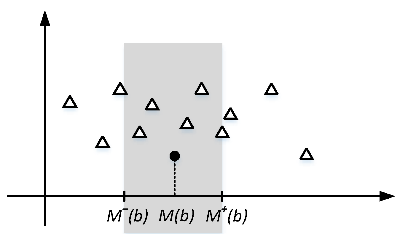
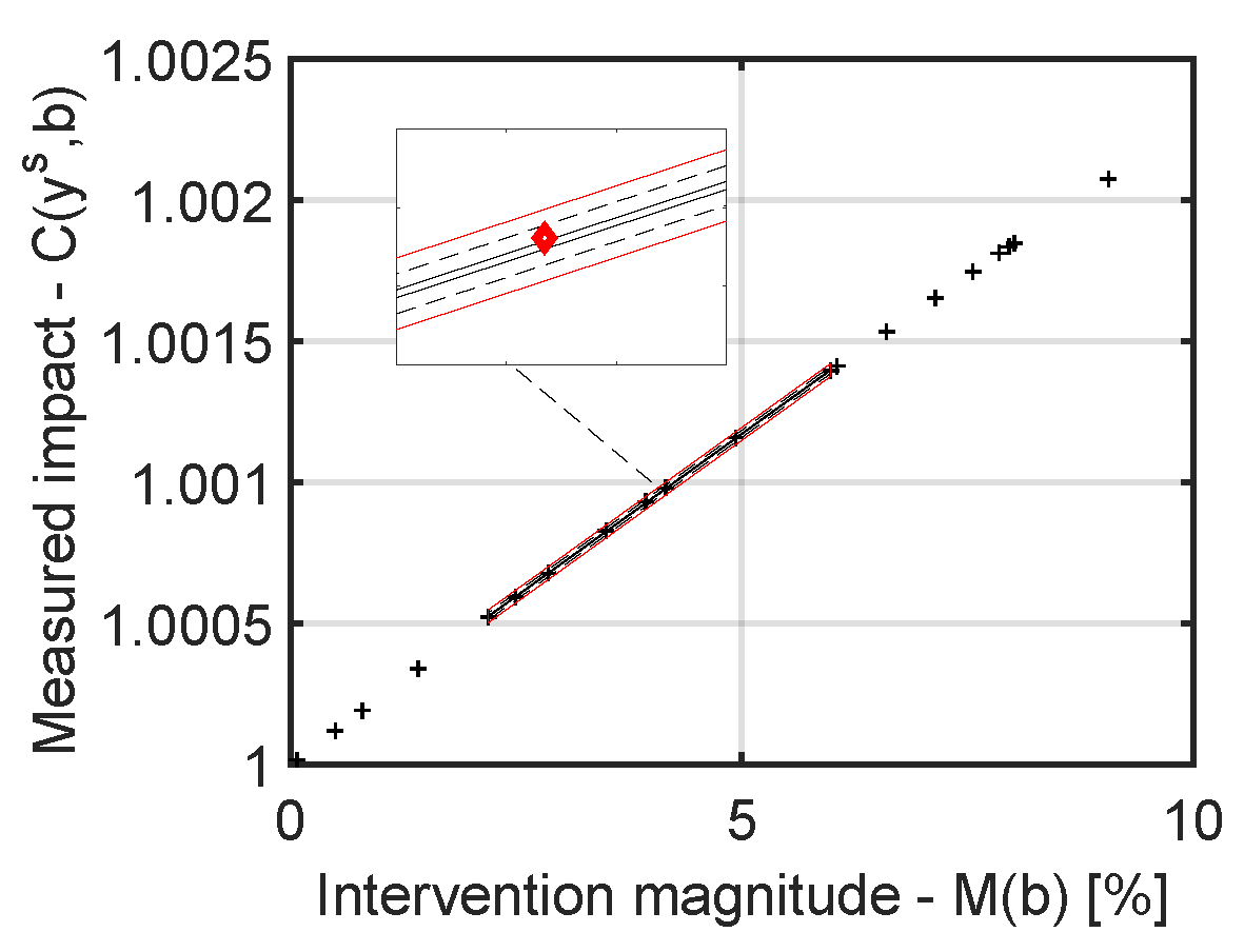
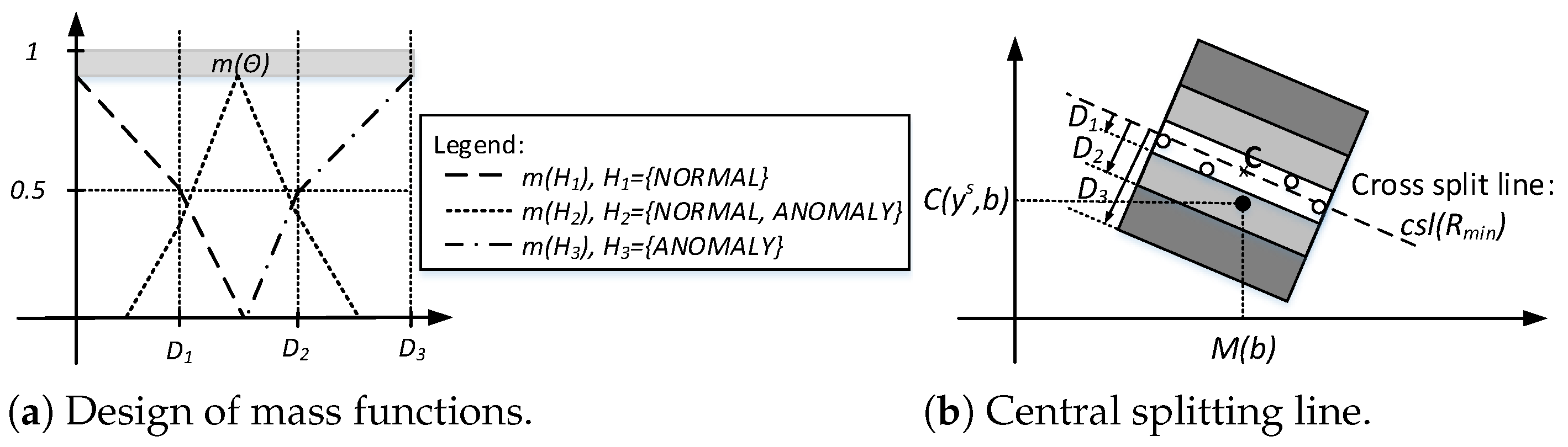
According to the D-S theory of evidence, we develop a fusion framework for detecting abnormal behavior, which could also be an indicator of the presence of an APT. According to D-S, we use $\mathsf{\Theta }$ to denote the set of all possible states upon which detectors have the ability to express certain evidence. We presume that each detector can express its belief in each of the system states.

For simplicity and clarity of presentation, we presume that for each observable variable, there is a detector in place. The frame of discernment $\mathsf{\Theta }$ is assumed to include three states, namely, ANOMALY, NORMAL, and $\mathsf{\Theta }$. Consequently, each detector needs to express its belief on a particular hypothesis $H\subseteq 2^{\mathsf{\Theta }}$, and on $\mathsf{\Theta }$. We use $m\left(\mathsf{\Theta }\right)$ to express the degree of uncertainty associated with a particular detector.

A significant aspect of the D-S framework is the definition of the mass function. For this purpose, expert knowledge can be included in order to model the output of the mass function. However, to aid the procedure, we develop an approach that uses the k Nearest Neighbours (kNN) for regression computation, and embrace expert knowledge for parameter estimation. In the following, the steps for the definition of mass functions are detailed.

• Step 1. For a new behaviour $b^{\prime }$ that is to be attested, let $M\left(b^{\prime }\right)$ denote the magnitude of the intervention, and $C(y^s,b^{\prime })$ the computed impact. The value of $M\left(b^{\prime }\right)$ can be computed in various ways, a straightforward approach would be the sum of deviations of control variable values from their mean values. In other cases (e.g., where timing is relevant for instance), a combination of the timing of applying interventions on control variables, and their deviation, could also be used for this purpose. Next, to establish the value of k, we first assume that the magnitude of the attested intervention is comparable with apriorily learned neighbouring interventions. Accordingly, and, by leveraging expert knowledge on the attested infrastructure, the lower $M^{-}\left(b^{\prime }\right)$ and upper $M^{+}\left(b^{\prime }\right)$ bounds of $M\left(b^{\prime }\right)$ ($M^{-}\left(b^{\prime }\right)<M^{+}\left(b^{\prime }\right)$) are determined (see Figure 2). Then, the set of relevant points, that is, the set of values to be used in the attestation of this new intervention, is determined according to Equation (8):

  $$\begin{array}{c}\hfill R_{y^s{b}^{\prime }}=\left\{C(y^s,b)|M^{-}\left(b^{\prime }\right)\le M\left(b\right)\le M^{+}\left(b^{\prime }\right),\forall b\in {\mathcal{B}}^s\right\}.\end{array}$$

  (8)
  According to the equation above, k equals the number of elements in $R_{y^s{b}^{\prime }}$.
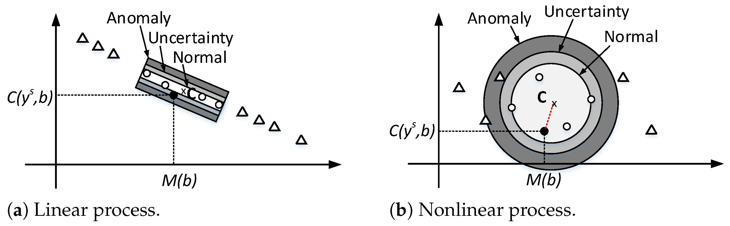
• Step 2. In the next phase, the coordinates of the centroid C given by the values in $R_{y^s{b}^{\prime }}$ are determined:

  $$\begin{array}{c}\hfill {\mathbf{C}}_x=\frac{1}{k}\sum _{b\in {\mathcal{B}}^s}M\left(b\right),\mathrm{where}C(y^s,b)\in R_{y^s{b}^{\prime }},\\ \hfill {\mathbf{C}}_y=\frac{1}{k}\sum _{b\in {\mathcal{B}}^s}C(y^s,b).\end{array}$$

  (9)
• Step 3. This last step determines the values for the mass functions for each hypothesis H. Unfortunately, various types of processes exhibit different behaviour. Some processes exhibit an approximately linear behaviour (considering possible measurement inaccuracies, and random noise), while others have a nonlinear behaviour. For each case, the estimate of the mass function should be particularly adapted.

In order to ease the design of the mass function, we illustrate two cases that could be applicable. For example, in the case of a linear process, the coordinates of the centroid C computed in the previous step represent the center of several rectangles. As shown in Figure 3a, the white rectangle is the minimal bounding box that encapsulates all the k selected values. Accordingly, a new value that fits within the area of this rectangle is associated with normal behaviour. A second rectangle with the same center as the previous one, but with larger sides, yields the uncertainty area. Lastly, outside the area of the two priorly mentioned rectangles values are considered to be anomalous.

Conversely, in the case of a nonlinear process, the coordinates of the centroid C may be given by the center of several circle-like shapes. As shown in Figure 3b, similarly to the linear case, we consider three shapes, where the radius of each shape determines the association of a new measurement to a particular state.

Considering the various opportunities to build the mass function, and also taking into account the particular behaviour of the physical process, we assume that $\mathcal{F}$ denotes the function that returns the allocation of a new attested value to a particular state: ANOMALY, NORMAL, and $\mathsf{\Theta }$ (for uncertainty). According to this allocation, the probability assignment for each hypothesis changes with the identified state.

As a last step, the fusion system applies the D-S rules to combine independent evidence from the implemented detectors. Since each intervention b yields a different system behaviour, and consequently, attestation result, a two-level fusion system is envisioned: Level 1 fuses decisions from individual detectors; and Level 2 fuses the decisions output by Level 1 associated to each intervention $b\in {\mathcal{B}}^s$.

3.4. Attestation Cost

Interventions, such as the ones described as part of the proposed attestation scheme, may have certain costs. For instance, in the case of the power plant model shown in Figure 1, a slight increase in the opening of the fuel valve, even for a brief time period, can increase costs in terms of used products (e.g., fuel and water), but also in terms of operational costs. However, we note that the developed methodology builds on quantifying the sensitivity of the process to certain changes. As a result, these changes may also be negative in the sense that reducing input material (e.g., by closing the feed valve) is also an option for applying the proposed methodology. Nevertheless, even in this case, there can be plant-specific operational costs that need to be taken into account while performing the attestation.

Accordingly, for ${\$}_{Prod}^b$ and ${\$}_{Op}^b$ denoting the cost of products and the costs of operations for performing attestation in scenario b, respectively, the total cost of the attestation is expressed via the following equation:

$$\begin{array}{c}\hfill {\$}_{ATT}=\sum _{s\in \mathcal{S}}\sum _{b\in {\mathcal{B}}^s}\left({\$}_{Prod}^b+{\$}_{Op}^b\right).\end{array}$$

(10)

3.5. APT Detection Time Reduction

The reduction in detection time provided by the developed methodology can be estimated as follows. We presume that the process is in the behavioural scenario $b_1$ at time $t_1$. Furthermore, we assume a subsequent behaviour $b_2$ that the process will exhibit in the future at time $t_2$. Since observation-based anomaly detection techniques require certain dynamics that would be expected in the transition from $b_1$ to $b_2$, an APT, in the best-case scenario may be detected at the moment of this transition. As a result, in the worst-case scenario, the improvement in the detection time brought by the developed technique is estimated to be at least $t_2-t_1$. Obviously, a more precise estimation requires a case-by-case assessment.

3.6. Analysis on the APT’s Advantage

We presume that an APT is considered successful in the case that the output of the level 2 fusion attributes the most mass value to the NORMAL hypothesis. Accordingly, let N denote the total number of detectors, where (for simplicity) we assumed that each detector is configured to attest the behaviour of one observable variable. Then, let P denote the number of compromised observable variables. We use the term compromised detector to denote a detector that uses a compromised observable variable as its input. Subsequently, we use F to denote the remaining number of non-compromised (attack-free) detectors, such that $N=P+F$.

Since an attacker may wish to increase his chances of not being detected, then he/she will try to predict the next best value for a compromised observable variable. Therefore, the best scenario for an attacker is when the compromised detectors activate only the NORMAL and $\mathsf{\Theta }$ hypothesis. Subsequently, the remaining non-compromised detectors will output the actual detected system state ANOMALY, alongside $\mathsf{\Theta }$.

According to these assumptions, let $X_p^P=m_{1,2,P}$, $Z_p^P=m_{1,2,P}$ denote the P-th fusion on the attacker’s mass functions on hypothesis NORMAL, and, $\mathsf{\Theta }$, respectively. Let $Y_f^F=m_{1,2,F}$, $Z_f^F=m_{1,2,F}$ denote the F-th fusion on the clear (non-compromised) mass functions on hypothesis ANOMALY, and $\mathsf{\Theta }$, respectively. Then, by means of deduction, we obtained the following recursive formulas, which express the result of fusion on P compromised detectors:

$$\begin{array}{c}\hfill X_p^P=\sum _{i=1}^P{a}_i^P{X}_p^{P-i+1}{Z}_p^{i-1},\\ \hfill \mathrm{where}{a}_i^P=a_{i-1}^{P-1}+a_i^{P-1},\mathrm{and}{a}_{i-1}^{P-1}=0,\mathrm{if}P-1=0;a_i^{P-1}=1,\mathrm{if}P=i.\end{array}$$

(11)

Similarly, for the case of the non-compromised (attack-free) F detectors, we obtained the following equations:

$$\begin{array}{c}\hfill Y_f^F=\sum _{i=1}^F{b}_i^F{Y}_f^{F-i+1}{Z}_f^{i-1},\\ \hfill \mathrm{where}{b}_i^F=b_{i-1}^{F-1}+b_i^{F-1},\mathrm{and}{b}_{i-1}^{F-1}=0,\mathrm{if}F-1=0;b_i^{F-1}=1,\mathrm{if}F=i.\end{array}$$

(12)

Next, we fuse the two mass functions $X_p^P$ and $Y_f^F$ on all hypothesis obtaining the following final mass function ($m_f$, where $K=X_p^P{Y}_f^F$):

$$\begin{array}{c}\hfill m_f\left(\mathrm{NORMAL}\right)=\frac{1}{1-K}{X}_p^P{Z}_f^F,m_f\left(\mathrm{ANOMALY}\right)=\frac{1}{1-K}{Y}_f^F{Z}_p^P,\\ \hfill m_f\left(\mathsf{\Theta }\right)=\frac{1}{1-K}{Z}_p^P{Z}_f^F.\end{array}$$

(13)

The advantage of the attacker Avd(APT) is then defined as:

$$\begin{array}{c}\hfill \mathtt{Adv}\left(\mathtt{APT}\right)=m_f\left(\mathrm{ANOMALY}\right)-m_f\left(\mathrm{NORMAL}\right).\end{array}$$

(14)

Consequently, as long as $\mathtt{Avd}\left(\mathtt{APT}\right)>0$, the attack is not reported by the decision fusion system. Therefore, the following condition needs to hold:

$$\begin{array}{c}\hfill \frac{1}{1-K}{X}_p^P{Z}_f^F>\frac{1}{1-K}{Y}_f^F{Z}_p^P.\end{array}$$

(15)

By eliminating the fraction from the left and right sides we obtain the following simplified equation:

$$\begin{array}{c}\hfill X_p^P{Z}_f^F>Y_f^F{Z}_p^P.\end{array}$$

(16)

Subsequently, by replacing the specific values we obtain that:

$$\begin{array}{c}\hfill Z_f^F\sum _{i=1}^P{a}_i^P{X}_p^{P-i+1}{Z}_p^{i-1}>Z_p^P\sum _{i=1}^F{b}_i^F{Y}_f^{F-i+1}{Z}_f^{i-1}.\end{array}$$

(17)

The equation above shows that the advantage of the attacker is influenced by the precision of the compromised elements, as well as, by the number of compromised process outputs. However, we observe that a larger number of compromised elements ($P>F$) but with lower precision ($X_p^P<Y_f^F$) will have a negative impact on the attacker’s advantage. Therefore, the attacker needs to strive and achieve high precision for predicting the correct value of compromised variables. Otherwise, even for a large number of compromised components, the attack may still be reported.

3.7. Summary of the Attestation Algorithm

The steps of the attestation procedure have been summarized in Algorithm 1. Accordingly, its input consists of the attested subsystem $s\in \mathcal{S}$, the known behavioral scenarios (${\mathcal{B}}^s$), and the new behavioral scenarios ${\mathcal{B}}^{{}^{\prime }s}$ that are computed for attestation purposes. Note that, for initialization purposes, the impact matrices for ${\mathcal{B}}^s$ are computed according to the previous equations. Next, the attestation of the new behavioral scenarios ${\mathcal{B}}^{{}^{\prime }s}$ can be performed. According to Algorithm 1, the steps are performed for each $b^{\prime }\in {\mathcal{B}}^{{}^{\prime }s}$ and each $s\in \mathcal{S}$. Consequently, the more sub-systems and behavioral scenarios are attested, the procedure becomes more time-intensive. Note that the algorithm also summarizes the Level 1 and Level 2 fusion. Here, $m^1$ and $m^2$ are used to denote Level 1 and Level 2 fusion, respectively.  

Algorithm 1: Attestation procedure including Level 1 and Level 2 fusion

4. Results

A prototype of E-APTDetect was developed in Matlab. In the following, E-APTDetect’s performance is evaluated in the context of the Vinyl Acetate Monomer (VAM) process model [14] (see Figure 4).

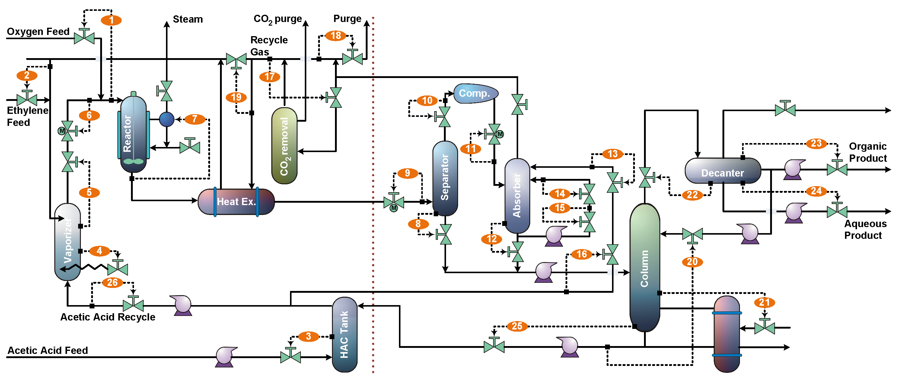
4.1. Process Description

The VAM process is a realistic model since VAM is a fundamental ingredient in a wide variety of industrial and consumer products including paints, adhesives, resins, and many other. It is the product of a large-scale chemical process consisting of several basic unit operations including: a vaporizer, a catalytic plug-flow reactor, a feed-effluent heat exchanger (FEHE), a vapor/liquid separator, a gas compressor, an absorber, a CO${}_2$ removal system, an azeotropic distillation column with a decanter, and a tank for the liquid recycle stream. The VAM is produced starting from fresh and recycled Ethylene (C${}_2$H${}_4$), Oxygen (O${}_2$), and acetic acid (HAc). These are converted into vinyl acetate, producing as byproducts the water (H${}_2$O) and carbon dioxide (CO${}_2$) components. The fresh C${}_2$H${}_4$ stream is combined with an inert C${}_2$H${}_6$ component.

The following equations describe the functionality of the VAM:

$$\begin{array}{c}\hfill C_2{H}_4+C{H}_{3}COOH+1/2O_2\to C{H}_2=CHOCOC{H}_3+H_{2}O,\\ \hfill C_2{H}_4+3O_2\to 2C{O}_2+2H_{2}O.\end{array}$$

(18)

For a detailed process description, readers are referred to [14]. According to [14], the VAM process is subject to two essential safety constraints:

• The oxygen composition must not exceed 8 mol% in the gas recycle loop. This is needed so that the process remains outside the explosivity envelope of ethylene;
• The pressure in the gas recycle loop and distillation column cannot exceed 140 psia because of the mechanical construction limit of the process vessels.

The VAM model has been made available to a broader audience by Rong Chen et al. [39] in the form of Matlab code. It includes 246 states, 26 control variables, and 43 observed variables. Readers are referred to [39] for a complete description of the model. Figure 4 depicts the main components and control loops of the VAM process.

Figure 5 depicts the normal operation of the VAM process (VAMP) based on a selection of two observed variables. It can be seen that the process exhibits two major states: an initialization phase, followed by a stable state.

4.2. Scenario Attestation

4.2.1. Scenario Description

Roughly, the VAM process can be divided into two sub-systems: reaction and refinement. The reaction part generates the main components (vinyl acetate), while the refinement is responsible for the distillation of the vinyl acetate product such that it meets certain quality specifications. We demonstrate the developed methodology by considering the first sub-system, which is found on the left side of the vertical dashed line shown in Figure 4. The scenario comprises the measurements related to the following components: Vaporizer, Reactor, Heat exchanger, CO₂ removal, and HAC Tank. In total, 18 measured (observed) variables are used.

In terms of behavioural scenarios, two scenarios have been selected. The first scenario involves changes on the ethylene feed valve (C${}_2$H${}_4$, control variable #2), and the second scenario includes changes on the acetic acid feed valve (HAC, control variable #3).

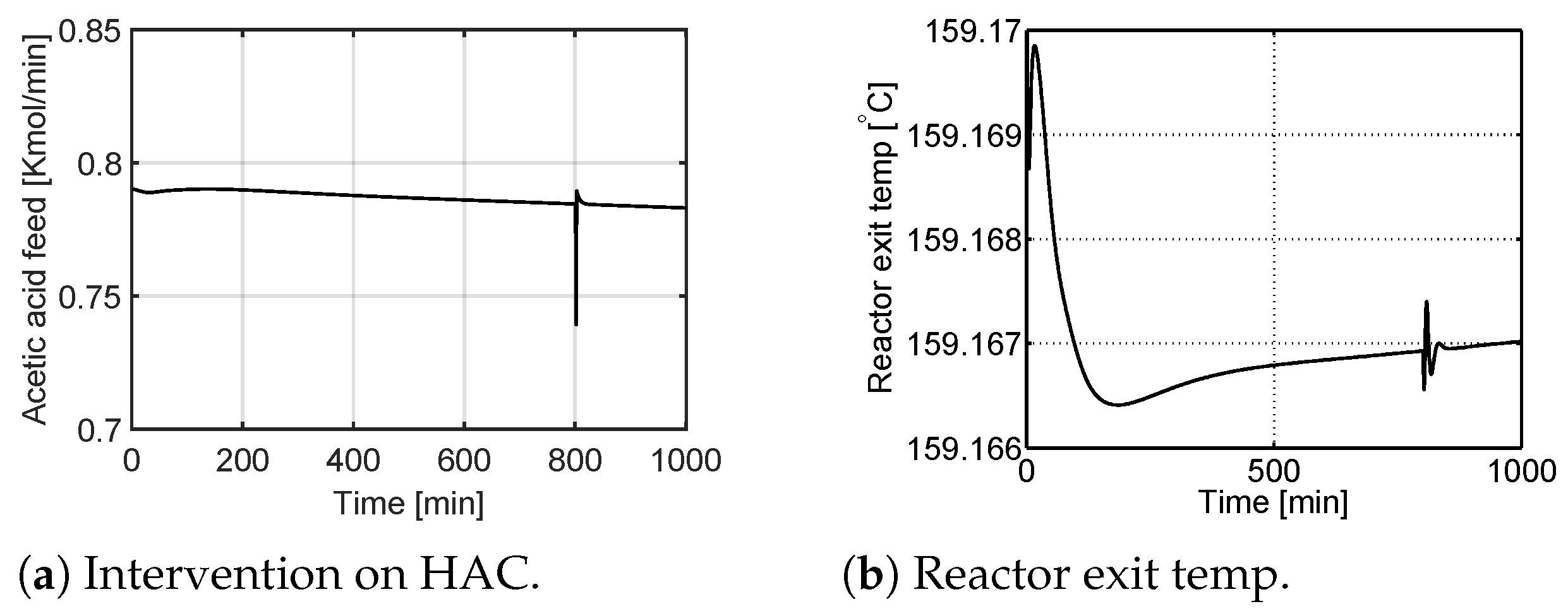
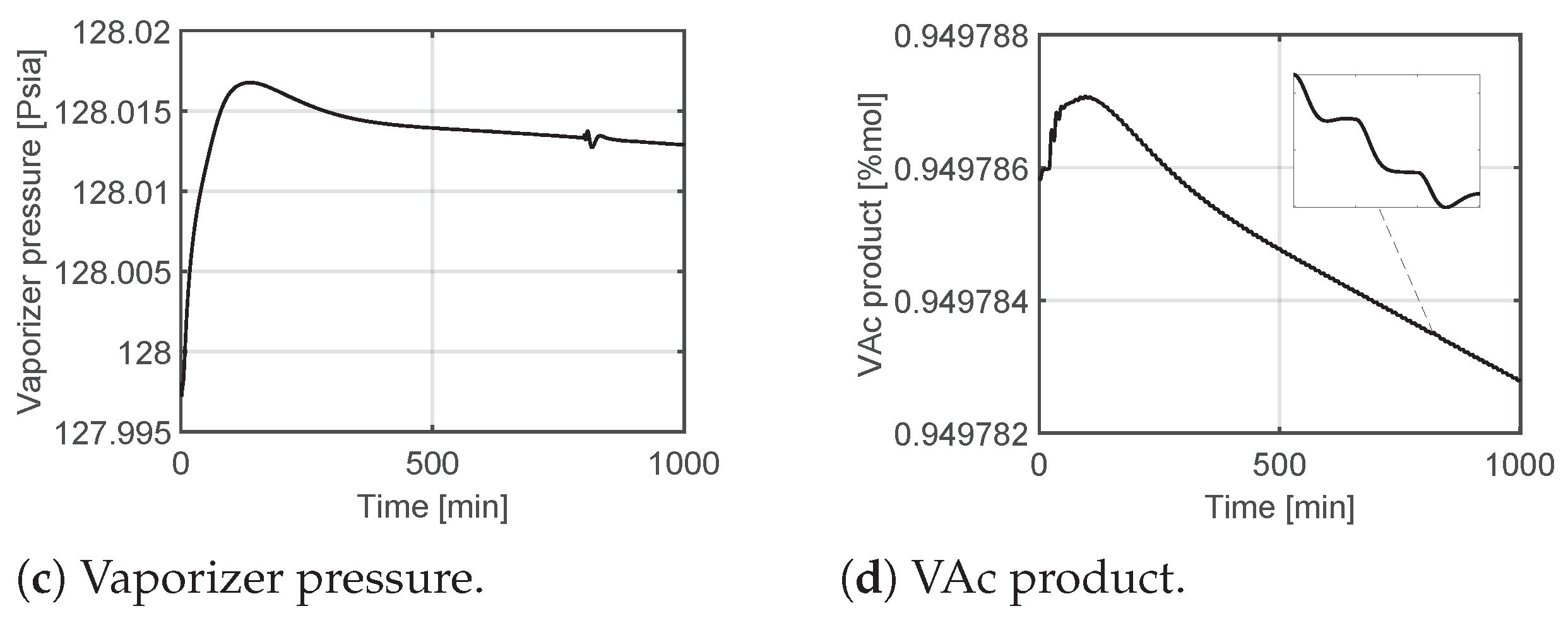
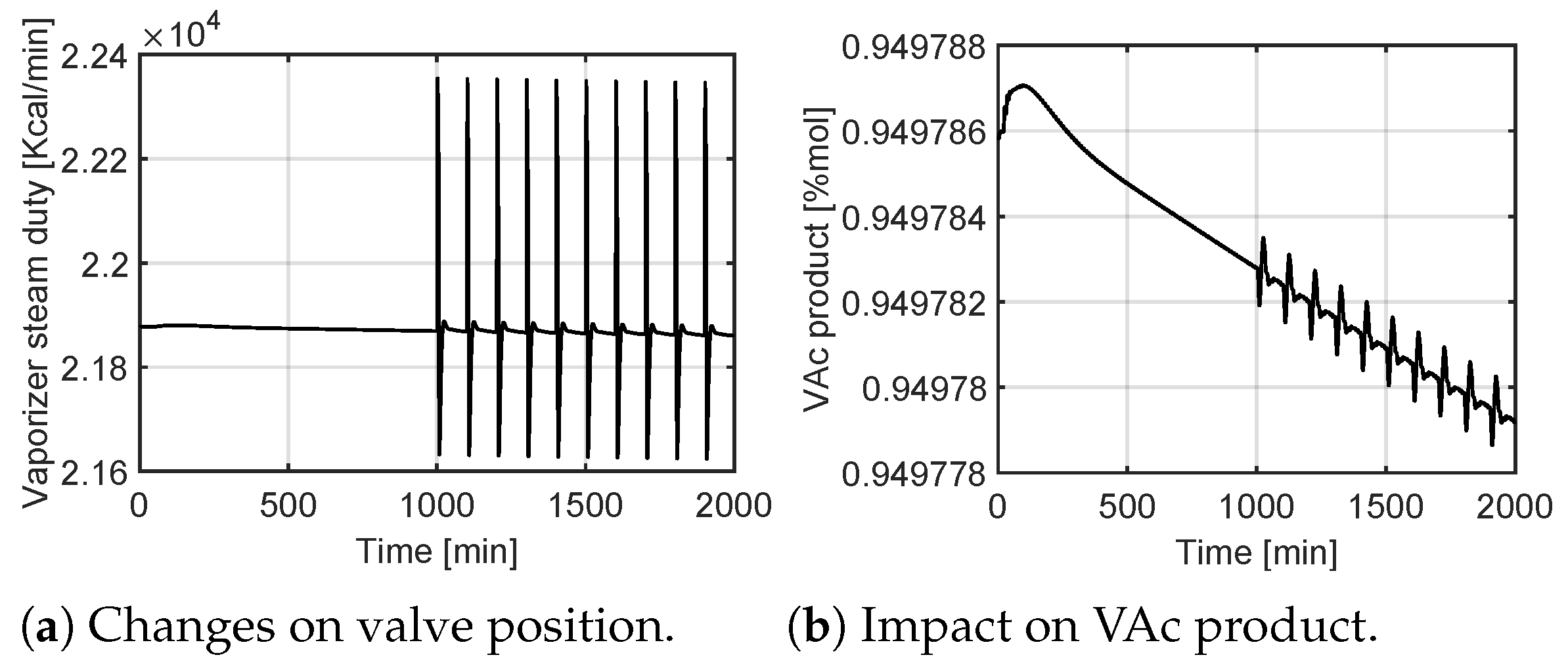
4.2.2. Intervention Example

First, a single intervention was triggered in the two selected scenarios (see Figure 6 and Figure 7). Accordingly, at 800 min within the simulation, a sudden change of 6% of the fed HAC and C${}_2$H${}_4$ products was triggered for 1 min. This has led to minor changes in the value of observable variables. While this intervention is visible in the case of the shown variables, note that, as an absolute value, the intervention causes minor deviations (e.g., less than 1% in most cases). Subsequently, the impact on the production of vinyl acetate (VAc) is minor, and therefore, the cost of this attestation, at least from the required products, is negligible. Obviously, the operational costs (i.e., ${\$}_{Op}$) might be more meaningful considering the necessary preparations and the large number of involved components. Nevertheless, the benefits of attestation may outweigh the involved operational costs.

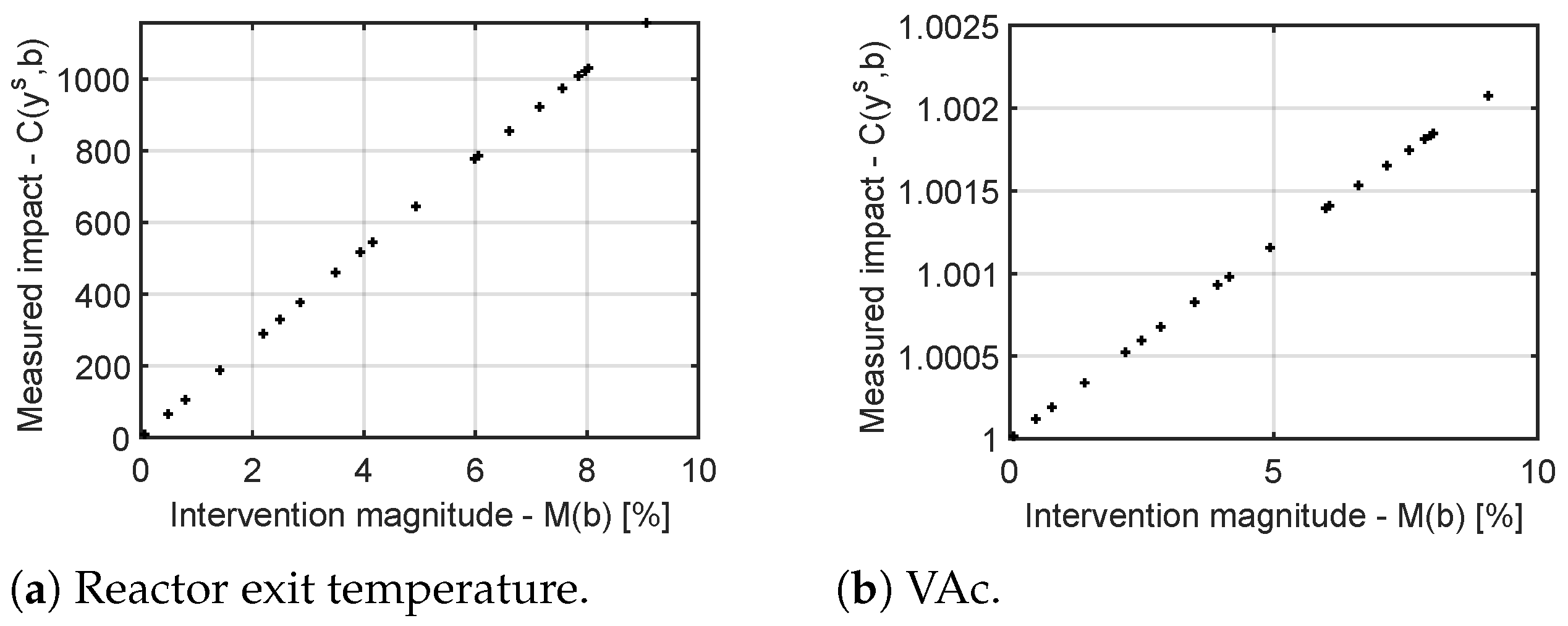
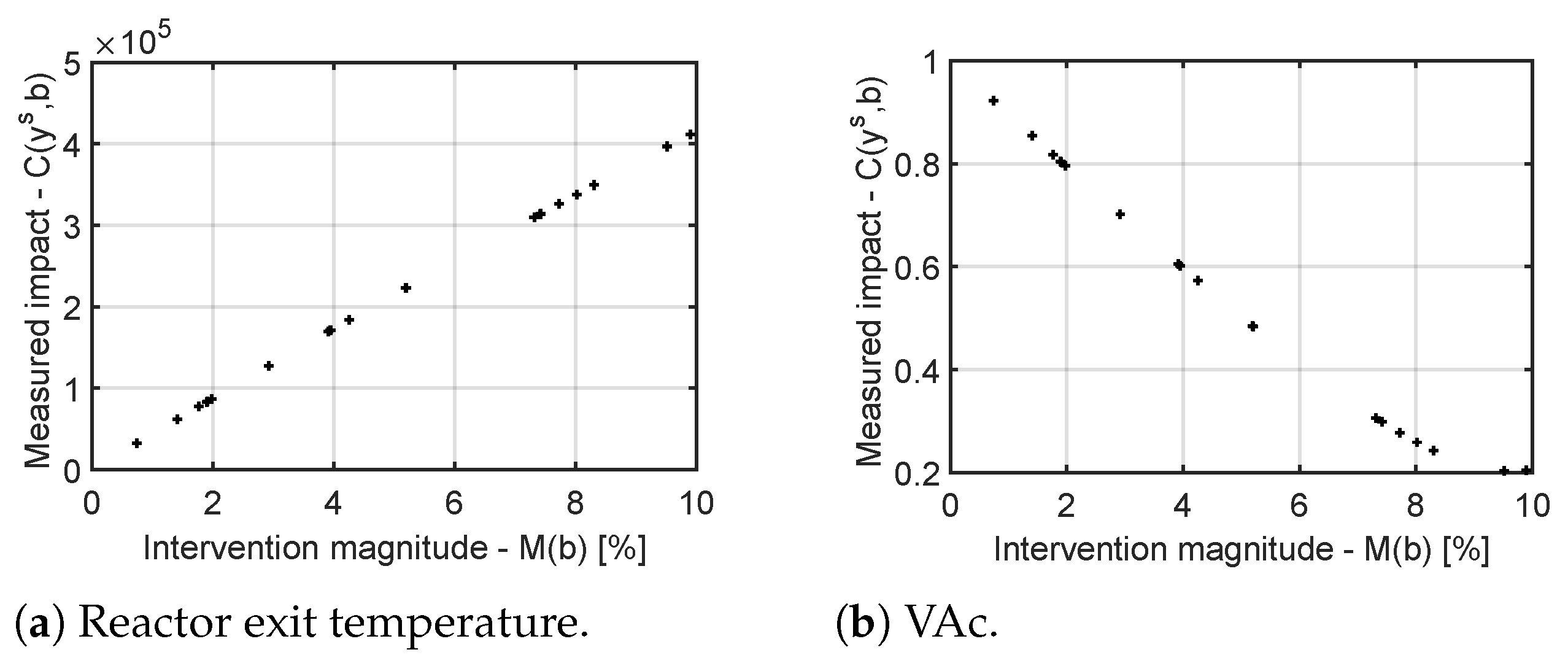
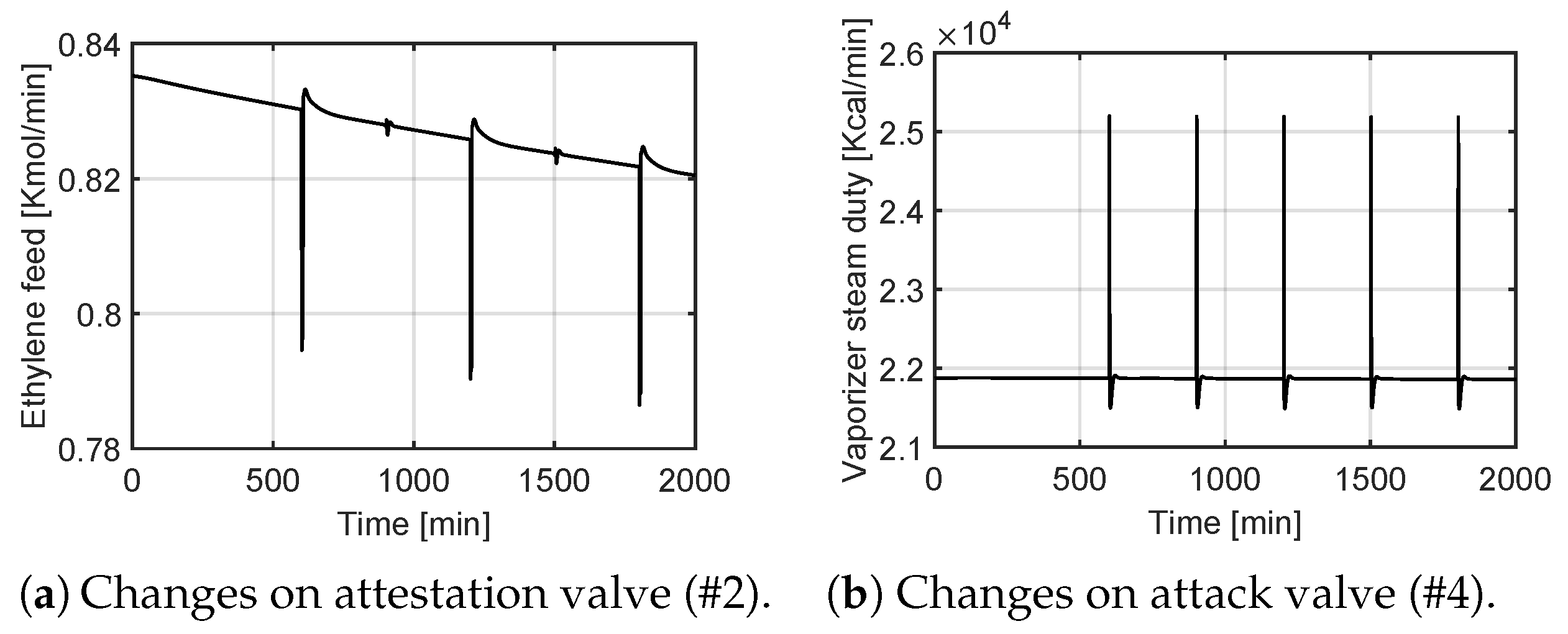
4.2.3. Random Interventions

In the next phase of the demonstration, for each of the two scenarios, we randomly performed 20 interventions, each one applying a slight decrease of the specific feed product (i.e., HAC and C${}_2$H${}_4$). In each of the cases, the change was limited to a maximum of 10% from the absolute value of the product and lasted for 1 min. For illustration purposes, we selected two observable variables from each of the two scenarios. In the case of the intervention on the HAC product, as shown in Figure 8a, the process exhibited a linear relation with respect to the intervention magnitude. As shown here, for each intervention of a particular magnitude ($M\left(b\right)$) the impact $C(y^s,b)$ was computed. The end result is a linear correspondence for all involved observable variables. Note that within these experiments the magnitude of intervention constitutes the deviation that is applied in %.

A similar behaviour was observed in the case of interventions on the C${}_2$H${}_4$ feed valve. As illustrated in Figure 9a, once again, the reactor exit temperature, and the VAc (as well as all the other observable variables) exhibit linear behaviour. In this case, however, the VAc shows a linear, yet inverse behaviour, compared to the interventions on HAC.

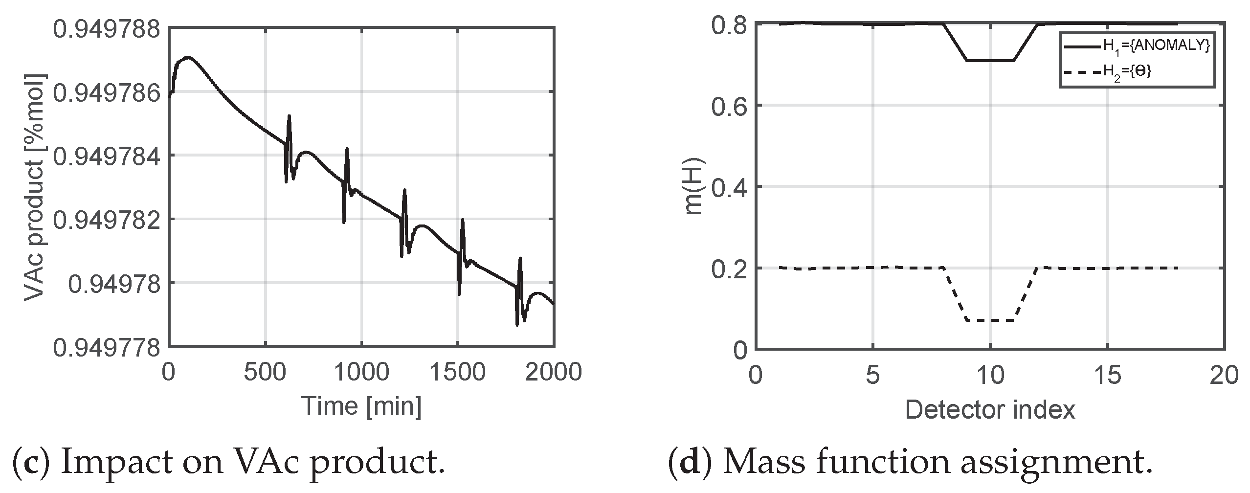
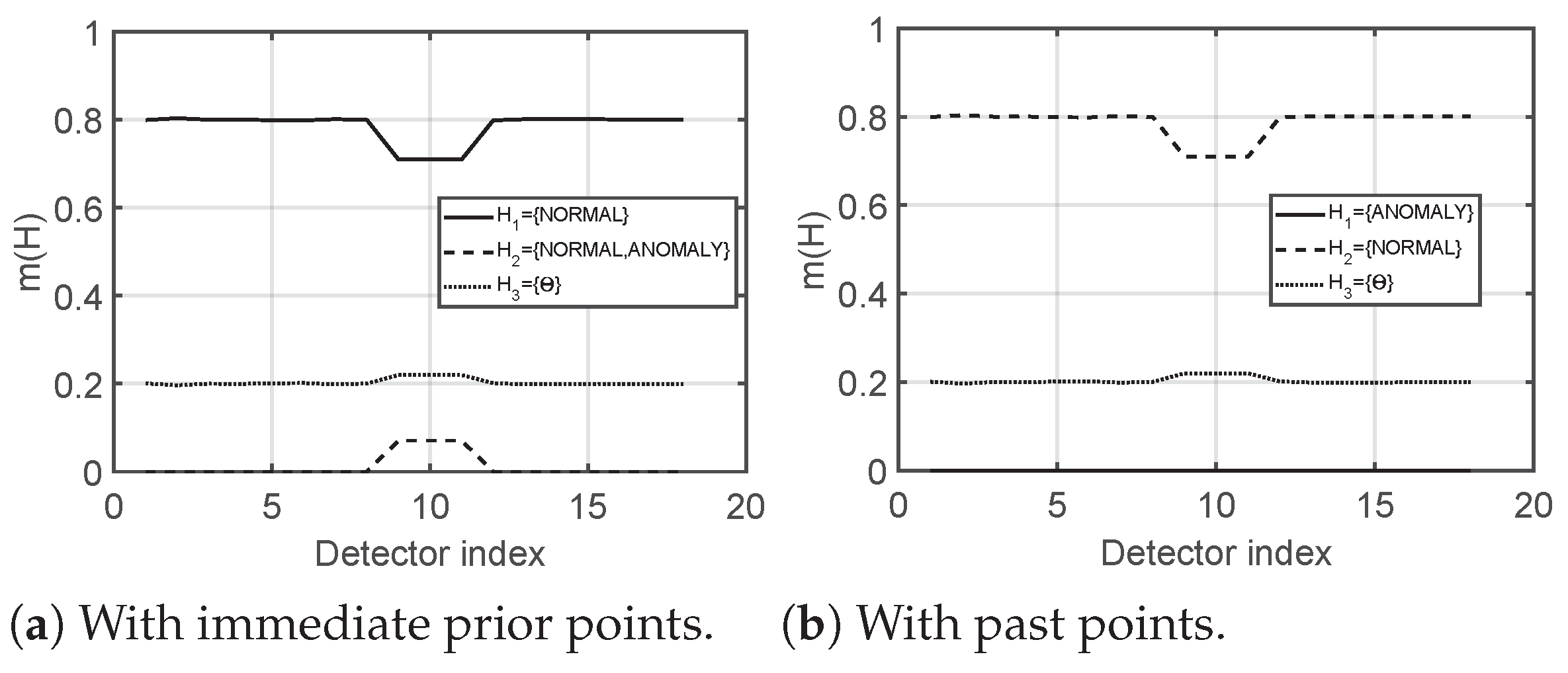
4.2.4. Constructing the Mass Functions

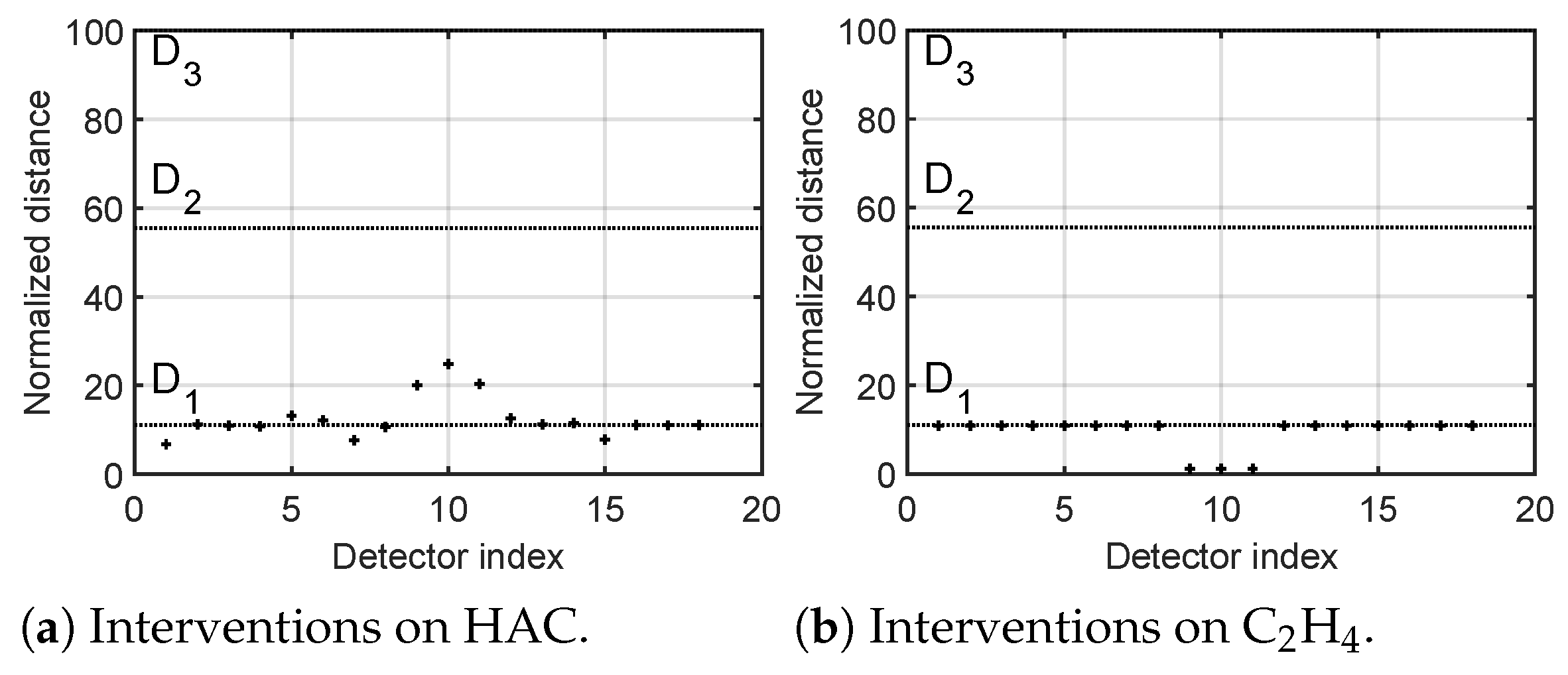
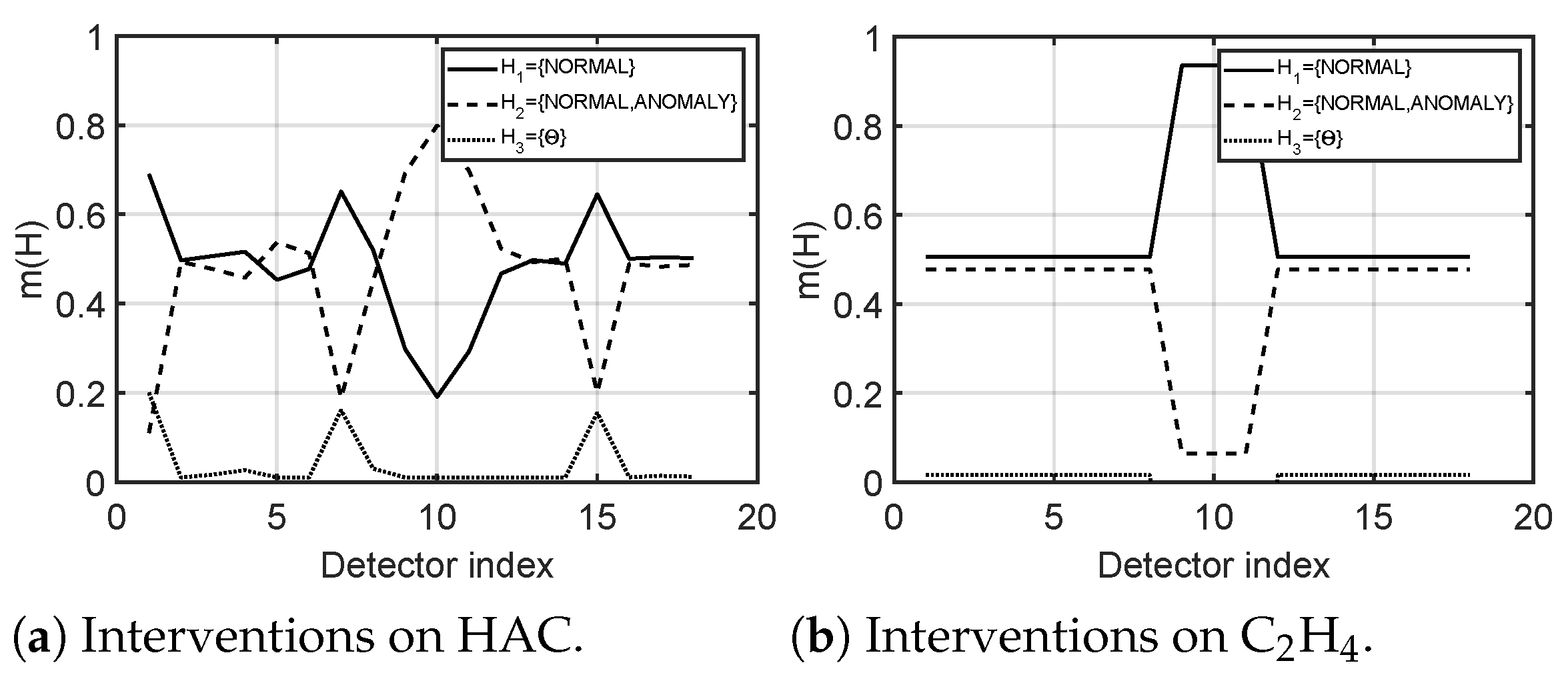
Moving forward, we demonstrate the construction of the mass functions for the process at hand. The first observation, as already mentioned, is the linear dependency between interventions and the computed impact matrix. Hence, we proceed to the selection of the $M^{-}\left(b^{\prime }\right)$ and upper $M^{+}\left(b^{\prime }\right)$ bounds for attestation. For demonstration purposes we select $M^{-}\left(b^{\prime }\right)=2$% and $M^{+}\left(b^{\prime }\right)=6$%. The interval bounded by these values provides six available interventions. Let V denote the set of interventions. Then, for each observed variable, we compute the three bounding rectangles that fit these interventions, similarly to the procedure shown in Figure 3a. Let $R_{min}\left(V\right)$ denote the minimum bounding rectangle that bounds the set of values V and has centroid C${}_{min}$. Let $h,w$ denote the height and width of the rectangle, respectively.

Subsequently, the uncertainty bounding rectangle denoted by $R_{unc}\left(V\right)$ contains $R_{min}\left(V\right)$, and therefore has the same centroid C${}_{min}$. Let $h_{unc},w_{unc}$ denote the height and width of the uncertainty rectangle, respectively. For the purposes of this experiment, we assume that $h_{unc}=3h$ and that $w_{unc}=w$, which means that the width of the uncertainty rectangle does not change. However, the height of this rectangle includes values that deviate at most two times from previous measurements. Obviously, these limits can be adjusted according to the process characteristics and measurement noise.

Similarly, we construct the anomaly bounding rectangle $R_{anom}\left(V\right)$, which contains $R_{min}\left(V\right)$, and has the same centroid C${}_{min}$. For $h_{anom},w_{anom}$ denoting the height and width of the uncertainty rectangle, respectively, $h_{anom}=5h$ and $w_{anom}=w$. An example illustration of the three bounding rectangles obtained for VAc with an intervention on the HAC feed valve is depicted in Figure 10.

In the next step, the translation to mass function assignments was performed. For this experiment, we assumed that $m\left(\mathsf{\Theta }\right)$ has the same value for all of the detectors, and its value is negligible (e.g., <0.001). Nevertheless, this value can be adjusted to express the level of confidence with respect to the reports originating from a particular detector.

An example design for the mass functions is provided in Figure 11a. Let $csl\left(\right)$ be a function that determines the central splitting line of a given rectangle, and $dist\left(\right)$ a function that returns the distance of a given point to a line segment. Subsequently, let $D_1=h/2$, $D_2=3h/2$, and $D_3=5h/2$ denote the distances from the central splitting line to the edge segment of each bounding box, as illustrated in Figure 11b. Let $(M\left(b\right),C(y^s,b))$ be a pair of intervention magnitude and the measured impact that requires attesting. Then, we compute $d=dist((M\left(b\right),C(y^s,b)),csl\left(R_{min}\right))$. According to the value of d with respect to distances $D_1,D_2$, and $D_3$, three cases are distinguished. For each case, the mass functions are obtained by projecting the distance d to each particular line segment that is active:

• Case 1. $d\le D_1$. Two hypothesis are active: $H_1$ = {NORMAL}, and $H_2$ = {NORMAL, ANOMALY}. The rationale for this is that as we move away from the center of $R_{min}$ the level of confidence in a normal state decreases, and, at the same time, we experience an increase in the level of uncertainty. In this case, the uncertainty is that the detector cannot distinguish between a normal and anomalous state.
• Case 2. $d\in (D_1,D_2]$. Three hypothesis are active: $H_1$ = {NORMAL}, $H_2$ = {NORMAL, ANOMALY}, and $H_3$ = {ANOMALY}. The rationale behind this decision is that, as we move further from $D_1$, we experience a decrease in the confidence of normality, while experiencing an increased confidence in uncertainty. Subsequently, starting from the middle of this interval the confidence in uncertainty begins to decrease as we proceed toward the $D_2$ limit. At the same time, the confidence assigned to an anomalous state begins to increase as we approach $D_2$.
• Case 3. $d>D_3$. Two hypothesis are active: $H_2$ = {NORMAL, ANOMALY}, and $H_3$ = {ANOMALY}. Similarly to the previous two cases, the rationale is that we experience a continuous decrease in the confidence in uncertainty, and, as we proceed towards $D_3$ the level of confidence increases for an anomalous state.

Note, however, that the depicted design of the mass functions can change according to particular processes, and the required decrease/increase speed for confidence level. For instance, $m\left(H_1\right)$ may exhibit a more rapid, exponentially inverse decrease in Case 2, which would express the lack of confidence in the normal state, while exponentially increasing the confidence in uncertainty.

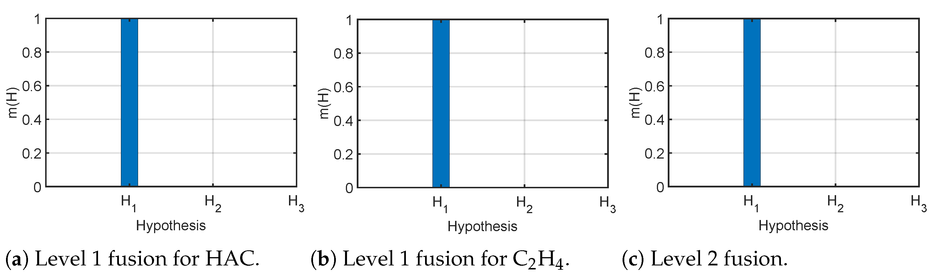
4.2.5. Level 1 and Level 2 Fusion

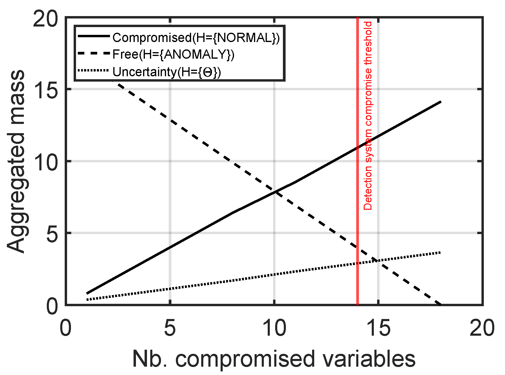
According to the experimental setting described earlier, we applied a new legitimate intervention to showcase the behaviour of the approach in the normal (legitimate) setting. Accordingly, the computed distance d for each of the detectors is illustrated in Figure 12a for interventions on HAC feed, and in Figure 12b for interventions on C${}_2$H${}_4$ feed. As shown here, the intervention on the HAC feed was found to be within the boundary of the $D_1$ distance. Nevertheless, in a few cases, the computed distance d exceeded this boundary, approaching the middle of the $(D_1,D_2]$ interval. A similar behaviour was observed in the C${}_2$H${}_4$ case. However, few detectors projected the new measurement closer to the center splitting line.

According to these values, in the next phase, each detector computed the mass function assignments to each hypothesis. The result has been illustrated in Figure 13a,b. Subsequently, the result of the level 1 fusion is shown in Figure 14a,b. In most of the cases, we observe that $H_1=NORMAL$ dominates the output results. However, there is uncertainty in a few cases regarding the system state. Nonetheless, none of the detectors activated the $H_3=ANOMALY$ hypothesis. In this case, the result of the level 2 fusion is obvious. The three hypotheses are preserved, while the system clearly outputs the absence of APT (Figure 14c).

4.3. APT Detection

In the next phase of the assessment, we showcase the behaviour of the developed detection system via synthetically generated APT behaviour. As documented by M. Krotofil in [40], in the particular case of the VAM process, an attacker may periodically manipulate certain variables for various reasons. In one of the described scenarios, Krotofil shows that periodically injected pulses (e.g., increase followed by decrease) on specially chosen control variables may have a significant economical impact. For example, according to [40], the repeated pulse on the vaporizer steam duty valve (control variable #4) may yield an economic loss of at least $10,000.

To showcase the effectiveness of the developed detection system, and to analyze the advantage of the APT, we leverage the intervention on the vaporizer steam duty valve, as described in [40]. The behaviour exhibited by this input is shown in Figure 15a. However, the impact of the repeated opening/closing of the valve may be visible on observable variables (Figure 15b). Therefore, the attacker may need to compromise a large number of observable variables to ensure that the input of each detector is according to the expected value.

Next, we presume that, in parallel to the APT, periodically, attestation is performed on an attack-free control variable. Namely, attestation was performed on the ${\mathrm{C}}_2{\mathrm{H}}_4$ feed valve every 600 min, while the attacker performed an intervention every 300 min (see Figure 16a,b). The impact of these interventions on a selected output, namely the production of VAc, is illustrated in Figure 16c. In case the attacker does not hide his/her presence, all detectors will report an anomaly. This behaviour is depicted in Figure 16d.

However, as mentioned earlier, in the case of an APT, the attacker may be aware of the implemented monitoring and detection solutions. Therefore, he/she may try to compromise as many elements as possible. The extreme case when the attacker is able to compromise all output, and manipulate the value reported for all observable variables is shown in Figure 17. Here, two scenarios are explored: a first scenario in which the attacker uses recently reported legitimate measurements to estimate the value of observable variables (Figure 17a); and, a second scenario where past values are used in the attacker’s estimations (Figure 17b). In both cases, we presume that all variables have been compromised. In the first scenario, the system is unable to detect the APT. However, in the second scenario, the ANOMALY state is reported by most of the detectors. This is owed to the fact that more recent measurements better reflect the current process state than past ones.

Next, we empirically assessed the advantage of the attacker, as detailed in Equation (17). As mentioned earlier, the advantage of APT is affected by the number of compromised detectors, and by the precision of the manipulated variables. Figure 18 details the result of this experiment in the same contextual scenario (attacker controls input #4, while attester uses input #2). As shown here, while the attacker leverages immediate prior values to estimate the next output, there is still a level of uncertainty, that, accumulated, will require a larger number of compromised elements. According to this experiment, the attacker needs to compromise at least 14 components (out of 18) in order for the APT not to be detected. This is a significant result that confirms our previous observation according to which it is not sufficient for the attacker to compromise the majority of components. It must do so by leveraging high-quality logic that reproduces the behaviour of the underlying physical process.

4.4. Discussion

As demonstrated by the previous experiments, E-APTDetect comprises a proactive methodology for triggering certain behavior, and consequently, for the detection of APTs. Its main building block considers that APTs are able to compromise a large number of components, and that, in the extreme case, all observed variables may be under the attacker’s control. As a result, the adversary will hide its presence by recreating the process’s state by various techniques ranging from replaying previous values, to reproducing the process behaviour in case sufficient details are acquired [41].

To counteract such sophisticated threats, E-APTDetect leverages system dynamics. The approach presumes randomly triggered changes to control variables, which lead to process behavioral changes that are randomly distributed in time. Consequently, while an adversary may easily hide its presence in the case of a steady-state process, random changes may be difficult to predict, and consequently, to forge. As illustrated by Equation (17), the adversary’s advantage is influenced not only by the number of compromised components, but also by the quality of forged values. Accordingly, in case the attacker compromises a large number of components, but with a reduced quality (i.e., low precision of forging observable variables), this will have a negative impact on the attacker’s advantage. Conversely, the adversary should strive to produce high-quality observable values to ensure stealthiness. For this purpose the adversary may need to observe and analyse the process behavior for a long time period; to identify the process state; and, to use highly accurate process models. Essentially, the APT’s success may be reduced to the quality of the elements used to hide the attacker’s presence.

While certain doubts may be raised about using process models in E-APTDetect’s validation, we observe that throughout the scientific literature, the use of simulation is a well-known technique to conduct security experiments [42,43,44]. Subsequently, considering the safety requirements for building such testbeds [44], process models represent an ideal candidate for such purposes. We further note that, the VAM process is a complex and large-scale model of a realistic physical system. As already stated, the process exhibits 246 states, 26 control variables, and 43 observed variables, which provides a complex environment for conducting a wide variety of experiments. Obviously, the output of the experiments needs to be interpreted within the process limitations and safety constraints. Nonetheless, the aim of E-APTDetect’s interventions is not to generate severe deviations in the process state, but to cause minor changes, which do not alter the process state, and ensure process execution within safety limitations. As a result, the output of the VAM process considering the defined interventions and experimental results can be considered as close to reality as the model is.

In terms of applications of E-APTDetect to real systems, a critical aspect is safety. Therefore, the interventions need to be defined by process experts such that these do not cause significant process deviations and are within the process safety limitations. Subsequently, since interventions will generate certain costs, the attestation costs, as defined in Equation (10) need to be estimated. As mentioned earlier, the estimated costs encapsulate the costs of products and operations required for performing the attestation. Considering also the complexity of the procedure, as exhibited in Algorithm 1, a higher number of behavioral scenarios and attested subsystems can further raise the attestation costs. Consequently, the application of E-APTDetect in the context of a real industrial system requires careful planning performed by process experts that take into account both the costs and system safety.

5. Conclusions

This paper documented the building blocks of E-APTDetect; a methodology for the early detection of APTs. At its core, E-APTDetect embraces sensitivity analysis as an approach to dynamic attestation of physical processes. On top of this, E-APTDetect uses Dempster-Shafer’s Theory of Evidence in order to fuse the evidence obtained via dynamic attestation. Experiments performed on a Vinyl Acetate Monomer (VAM) process model demonstrated the effectiveness of the developed approach, while they also highlighted that the adversary’s advantage is affected by two major factors: the number of compromised components; and, the precision of manipulation. It was shown that, while an attacker may compromise most components, its success is only guaranteed if the manipulated variables exhibit a high precision in replicating the process behaviour. Otherwise, in case an adversary uses priorly recorded values, its presence would be immediately detected and reported. As part of future work, a prototype implementation will be developed and assessed in the context of a laboratory environment. Subsequently, E-APTDetect will be applied to a broader range of processes in order to establish its generality (e.g., power systems, water supply systems). Additional future research directions may constitute investigation of the application of neural networks, and nature-inspired techniques for the detection of and adaptive defense against APTs.

References

1. Hagerott, M. Stuxnet and the vital role of critical infrastructure operators and engineers. Int. J. Crit. Infrastruct. Prot. 2014, 7, 244–246. [Google Scholar] [CrossRef]
2. Turton, W.; Mehrotra, K. Hackers Breached Colonial Pipeline Using Compromised Password. 2021. Available online: https://www.bloomberg.com/news/articles/2021-06-04/hackers-breached-colonial-pipeline-using-compromised-password (accessed on 5 March 2023).
3. MacKenzie, H. How Dragonfly Hackers and RAT Malware Threaten ICS Security. 2014. Available online: https://www.belden.com/blogs/industrial-security/how-dragonfly-hackers-and-rat-malware-threaten-ics-security (accessed on 5 March 2023).
4. Genge, B.; Graur, F.; Haller, P. Experimental assessment of network design approaches for protecting industrial control systems. Int. J. Crit. Infrastruct. Prot. 2015, 11, 24–38. [Google Scholar] [CrossRef]
5. Alshamrani, A.; Myneni, S.; Chowdhary, A.; Huang, D. A Survey on Advanced Persistent Threats: Techniques, Solutions, Challenges, and Research Opportunities. IEEE Commun. Surv. Tutor. 2019, 21, 1851–1877. [Google Scholar] [CrossRef]
6. Bolboacă, R. Adaptive Ensemble Methods for Tampering Detection in Automotive Aftertreatment Systems. IEEE Access 2022, 10, 105497–105517. [Google Scholar] [CrossRef]
7. Huang, L.; Zhu, Q. A dynamic games approach to proactive defense strategies against Advanced Persistent Threats in cyber-physical systems. Comput. Secur. 2020, 89, 101660. [Google Scholar] [CrossRef] [Green Version]
8. Rubio, J.E.; Roman, R.; Alcaraz, C.; Zhang, Y. Tracking Advanced Persistent Threats in Critical Infrastructures Through Opinion Dynamics. In Proceedings of the European Symposium on Research in Computer Security, ESORICS 2018, Barcelona, Spain, 3–7 September 2018; Lopez, J., Zhou, J., Soriano, M., Eds.; Springer International Publishing: Cham, Switzerland, 2018; pp. 555–574. [Google Scholar] [CrossRef]
9. Rubio, J.E.; Roman, R.; Lopez, J. Integration of a Threat Traceability Solution in the Industrial Internet of Things. IEEE Trans. Ind. Inform. 2020, 16, 6575–6583. [Google Scholar] [CrossRef]
10. Neuschmied, H.; Winter, M.; Stojanović, B.; Hofer-Schmitz, K.; Božić, J.; Kleb, U. APT-Attack Detection Based on Multi-Stage Autoencoders. Appl. Sci. 2022, 12, 6816. [Google Scholar] [CrossRef]
11. Sathya, M.; Jeyaselvi, M.; Krishnasamy, L.; Hazzazi, M.M.; Shukla, P.K.; Shukla, P.K.; Nuagah, S.J. A novel, efficient, and secure anomaly detection technique using DWU-ODBN for IoT-enabled multimedia communication systems. Wirel. Commun. Mob. Comput. 2021, 2021, 4989410. [Google Scholar] [CrossRef]
12. Forrester, J.W. Counterintuitive behavior of social systems. Theory Decis. 1971, 2, 109–140. [Google Scholar] [CrossRef]
13. Genge, B.; Kiss, I.; Haller, P. A system dynamics approach for assessing the impact of cyber attacks on critical infrastructures. Int. J. Crit. Infrastruct. Prot. 2015, 10, 3–17. [Google Scholar] [CrossRef]
14. Luyben, M.L.; Tyreus, B.D. An industrial design/control study for the vinyl acetate monomer process. Comput. Chem. Eng. 1998, 22, 867–877. [Google Scholar] [CrossRef]
15. Filippini, R.; Silva, A. A modeling framework for the resilience analysis of networked systems-of-systems based on functional dependencies. Reliab. Eng. Syst. Saf. 2014, 125, 82–91. [Google Scholar] [CrossRef]
16. Giani, A.; Bent, R.; Pan, F. Phasor measurement unit selection for unobservable electric power data integrity attack detection. Int. J. Crit. Infrastruct. Prot. 2014, 7, 155–164. [Google Scholar] [CrossRef] [Green Version]
17. Rubio, J.E.; Alcaraz, C.; Roman, R.; Lopez, J. Analysis of Intrusion Detection Systems in Industrial Ecosystems. In Proceedings of the 14th International Joint Conference on e-Business and Telecommunications (ICETE 2017)—Volume 4: SECRYPT, Madrid, Spain, 24–26 July 2017; pp. 116–128. [Google Scholar] [CrossRef]
18. Cárdenas, A.; Amin, S.; Lin, Z.; Huang, Y.; Huang, C.; Sastry, S. Attacks against process control systems: Risk assessment, detection, and response. In Proceedings of the 6th ACM Symposium on Information, Computer and Communications Security, ASIACCS 2011, Hong Kong, China, 22–24 March 2011; pp. 355–366. [Google Scholar] [CrossRef]
19. Giraldo, J.; Cardenas, A.; Quijano, N. Integrity Attacks on Real-Time Pricing in Smart Grids: Impact and Countermeasures. IEEE Trans. Smart Grid 2017, 8, 2249–2257. [Google Scholar] [CrossRef]
20. Carcano, A.; Coletta, A.; Guglielmi, M.; Masera, M.; Fovino, I.N.; Trombetta, A. A Multidimensional Critical State Analysis for Detecting Intrusions in SCADA Systems. IEEE Trans. Ind. Inform. 2011, 7, 179–186. [Google Scholar] [CrossRef]
21. Fovino, I.N.; Coletta, A.; Carcano, A.; Masera, M. Critical State-Based Filtering System for Securing SCADA Network Protocols. IEEE Trans. Ind. Electron. 2012, 59, 3943–3950. [Google Scholar] [CrossRef]
22. Kiss, I.; Genge, B.; Haller, P.; Sebestyén, G. Data clustering-based anomaly detection in industrial control systems. In Proceedings of the 2014 IEEE 10th International Conference on Intelligent Computer Communication and Processing (ICCP), Cluj-Napoca, Romania, 4–6 September 2014; pp. 275–281. [Google Scholar] [CrossRef]
23. Wang, B.; Mao, Z. One-class classifiers ensemble based anomaly detection scheme for process control systems. Trans. Inst. Meas. Control 2018, 40, 3466–3476. [Google Scholar] [CrossRef]
24. Ha, D.; Ahmed, U.; Pyun, H.; Lee, C.J.; Baek, K.H.; Han, C. Multi-mode operation of principal component analysis with k-nearest neighbor algorithm to monitor compressors for liquefied natural gas mixed refrigerant processes. Comput. Chem. Eng. 2017, 106, 96–105. [Google Scholar] [CrossRef]
25. Portnoy, I.; Melendez, K.; Pinzon, H.; Sanjuan, M. An improved weighted recursive PCA algorithm for adaptive fault detection. Control Eng. Pract. 2016, 50, 69–83. [Google Scholar] [CrossRef]
26. Chen, B.; Ho, D.W.C.; Zhang, W.A.; Yu, L. Distributed Dimensionality Reduction Fusion Estimation for Cyber-Physical Systems Under DoS Attacks. IEEE Trans. Syst. Man Cybern. Syst. 2017, 49, 455–468. [Google Scholar] [CrossRef]
27. Genge, B.; Haller, P.; Enăchescu, C. Anomaly Detection in Aging Industrial Internet of Things. IEEE Access 2019, 7, 74217–74230. [Google Scholar] [CrossRef]
28. Enăchescu, C.; Sándor, H.; Genge, B. A Multi-Model-based Approach to Detect Cyber Stealth Attacks in Industrial Internet of Things. In Proceedings of the 2019 International Conference on Software, Telecommunications and Computer Networks (SoftCOM), Split, Croatia, 19–21 September 2019; pp. 1–6. [Google Scholar] [CrossRef]
29. Zhao, J.; Zhang, G.; Jabr, R.A. Robust Detection of Cyber Attacks on State Estimators Using Phasor Measurements. IEEE Trans. Power Syst. 2017, 32, 2468–2470. [Google Scholar] [CrossRef]
30. Shoukry, Y.; Nuzzo, P.; Puggelli, A.; Sangiovanni-Vincentelli, A.L.; Seshia, S.A.; Tabuada, P. Secure State Estimation for Cyber-Physical Systems under Sensor Attacks: A Satisfiability Modulo Theory Approach. IEEE Trans. Autom. Control 2017, 62, 4917–4932. [Google Scholar] [CrossRef]
31. Huang, L.; Zhu, Q. Adaptive Strategic Cyber Defense for Advanced Persistent Threats in Critical Infrastructure Networks. ACM SIGMETRICS Perform. Eval. Rev. 2019, 46, 52–56. [Google Scholar] [CrossRef] [Green Version]
32. Hassannataj Joloudari, J.; Haderbadi, M.; Mashmool, A.; Ghasemigol, M.; Band, S.S.; Mosavi, A. Early Detection of the Advanced Persistent Threat Attack Using Performance Analysis of Deep Learning. IEEE Access 2020, 8, 186125–186137. [Google Scholar] [CrossRef]
33. Javed, S.H.; Ahmad, M.B.; Asif, M.; Almotiri, S.H.; Masood, K.; Ghamdi, M.A.A. An Intelligent System to Detect Advanced Persistent Threats in Industrial Internet of Things (I-IoT). Electronics 2022, 11, 742. [Google Scholar] [CrossRef]
34. Ghafir, I.; Hammoudeh, M.; Prenosil, V.; Han, L.; Hegarty, R.; Rabie, K.; Aparicio-Navarro, F.J. Detection of advanced persistent threat using machine-learning correlation analysis. Future Gener. Comput. Syst. 2018, 89, 349–359. [Google Scholar] [CrossRef] [Green Version]
35. Zimba, A.; Chen, H.; Wang, Z.; Chishimba, M. Modeling and detection of the multi-stages of Advanced Persistent Threats attacks based on semi-supervised learning and complex networks characteristics. Future Gener. Comput. Syst. 2020, 106, 501–517. [Google Scholar] [CrossRef]
36. Bell, R.; Åström, K. Dynamic Models for Boiler–Turbine Alternator Units: Data Logs and Parameter Estimation for a 160 MW Unit; Report TFRT–3192; Lundt Institute of Technology: Skåne, Sweden, 1987. [Google Scholar]
37. Huang, J.; Howley, E.; Duggan, J. The Ford Method: A Sensitivity Analysis Approach. In Proceedings of the Twenty-Seventh International Conference of the System Dynamics Society, Albuquerque, NM, USA, 26–30 July 2009; pp. 355–366. [Google Scholar]
38. Shafer, G. A Mathematical Theory of Evidence; Princeton University Press: Princeton, NJ, USA, 1976. [Google Scholar]
39. Chen, R.; Dave, K.; McAvoy, T.J. A Nonlinear Dynamic Model of a Vinyl Acetate Process. Ind. Eng. Chem. Res. 2003, 42, 4478–4487. [Google Scholar] [CrossRef]
40. Krotofil, M.; Larsen, J.W. Rocking the pocket book: Hacking chemical plants for competition and extortion. In Proceedings of the BlackHat; 2015. Available online: https://www.blackhat.com/us-15/briefings.html#marina-krotofil (accessed on 5 March 2023).
41. Haller, P.; Genge, B.; Forloni, F.; Baldini, G.; Carriero, M.; Fontaras, G. VetaDetect: Vehicle tampering detection with closed-loop model ensemble. Int. J. Crit. Infrastruct. Prot. 2022, 37, 100525. [Google Scholar] [CrossRef]
42. Oruc, A.; Gkioulos, V.; Katsikas, S. Towards a Cyber-Physical Range for the Integrated Navigation System (INS). J. Mar. Sci. Eng. 2022, 10, 107. [Google Scholar] [CrossRef]
43. Smadi, A.A.; Ajao, B.T.; Johnson, B.K.; Lei, H.; Chakhchoukh, Y.; Abu Al-Haija, Q. A Comprehensive Survey on Cyber-Physical Smart Grid Testbed Architectures: Requirements and Challenges. Electronics 2021, 10, 1043. [Google Scholar] [CrossRef]
44. Siaterlis, C.; Genge, B.; Hohenadel, M. EPIC: A Testbed for Scientifically Rigorous Cyber-Physical Security Experimentation. IEEE Trans. Emerg. Top. Comput. 2013, 1, 319–330. [Google Scholar] [CrossRef]
Figure 1. Example process of a boiling water power plant including control and measurement parameters.
Applsci 13 03409 g001
Figure 2. Selection of the k parameter for the kNN regression computation. The filled circle denotes a new behavior, while triangles denote priorly attested behavior.
Applsci 13 03409 g002
Figure 3. Example design of the mass function. Empty circles denote nearest neighbours, the new attested element is illustrated with a filled circle, and non-selected elements are denoted by triangles.
Applsci 13 03409 g003
Figure 4. The physical architecture of the Vinyl Acetate Monomer process (VAMP) and the associated control loops (illustrated by numbers).
Applsci 13 03409 g004
Figure 5. The normal operation of VAMP for two observed variables.
Applsci 13 03409 g005
Figure 6. Example intervention on the HAC feed valve (control variable #3), and its impact on a selection of observable variables.
Applsci 13 03409 g006aApplsci 13 03409 g006b
Figure 7. Example intervention on the C 2 H 4 feed product (control variable #2) and its impact on a selection of observable variables.
Applsci 13 03409 g007
Figure 8. Attestation result on two observable variables with intervention on the HAC feed product.
Applsci 13 03409 g008
Figure 9. Attestation result on two observable variables with intervention on the C 2 H 4 feed product.
Applsci 13 03409 g009
Figure 10. Example of attested measurement with intervention on the HAC. VAc is the observable variable.
Applsci 13 03409 g010
Figure 11. Example design of mass functions and central splitting.
Applsci 13 03409 g011
Figure 12. Computed mass function of each detector in the case of two interventions.
Applsci 13 03409 g012
Figure 13. Mass function assignment in two intervention scenarios.
Applsci 13 03409 g013
Figure 14. Level 1 and level 2 fusion result. In all cases H 1 = { N O R M A L } , H 2 = { N O R M A L , A N O M A L Y } , H 3 = { Θ } .
Applsci 13 03409 g014
Figure 15. APT example: repeated pulses on the vaporizer steam duty valve (control variable #4).
Applsci 13 03409 g015
Figure 16. APT and attestation example.
Applsci 13 03409 g016aApplsci 13 03409 g016b
Figure 17. Detectors input compromised by attacker’s estimation via linear regression.
Applsci 13 03409 g017
Figure 18. Progressive increase in the number of compromised detectors (compromised observable variables).
Applsci 13 03409 g018
Disclaimer/Publisher’s Note: The statements, opinions and data contained in all publications are solely those of the individual author(s) and contributor(s) and not of MDPI and/or the editor(s). MDPI and/or the editor(s) disclaim responsibility for any injury to people or property resulting from any ideas, methods, instructions or products referred to in the content.