A Novel Deep Learning Method for Predicting RNA-Protein Binding Sites

Abstract

The cell cycle and biological processes rely on RNA and RNA-binding protein (RBP) interactions. It is crucial to identify the binding sites on RNA. Various deep-learning methods have been used for RNA-binding site prediction. However, they cannot extract the hierarchical features of the RNA secondary structure. Therefore, this paper proposes HPNet, which can automatically identify RNA-binding sites and -binding preferences. HPNet performs feature learning from the two perspectives of the RNA sequence and the RNA secondary structure. A convolutional neural network (CNN), a deep-learning method, is used to learn RNA sequence features in HPNet. To capture the hierarchical information for RNA, we introduced DiffPool into HPNet, a differentiable pooling graph neural network (GNN). A CNN and DiffPool were combined to improve the binding site prediction accuracy by leveraging both RNA sequence features and hierarchical features of the RNA secondary structure. Binding preferences can be extracted based on model outputs and parameters. Overall, the experimental results showed that HPNet achieved a mean area under the curve (AUC) of 94.5% for the benchmark dataset, which was more accurate than the state-of-the-art methods. Moreover, these results demonstrate that the hierarchical features of RNA secondary structure play an essential role in selecting RNA-binding sites.

1. Introduction

RNA plays a critical role as a crucial carrier for genetic information [1,2]. RNA-binding proteins (RBPs) are essential regulators of various stages of cellular RNA, including RNA transcription, RNA translation, RNA editing, and mRNA localization [3,4]. An RBP contains at least one RNA-binding domain (RBD) [5]. It can recognize specific binding sites on RNA and form polymers with RNA, making it possible to regulate the expression of RNA functions [6,7,8]. More than 2000 RBPs have been identified [9], but only a few RBP processes are thoroughly understood. Mutations in genes, RNA function failure, and other issues are directly linked to aberrant combinations of RBP and RNA, which biological studies have shown to be a significant contributor to the development of many diseases. For example, IRP1 binding to FTL mRNA is disrupted by mutations in the iron-responsive region of the FTL gene, leading to hyperferritinemia-cataract syndrome [10,11]. Therefore, solving more complex biological problems requires a thorough understanding of RBP-binding sites and preferences. It is crucial to investigate the binding specificity between RBP and RNA.

With the advent of high-throughput sequencing technology, biological experiments have confirmed the binding RNAs and the binding sites of various RBPs [12,13]. Crosslinking and immunoprecipitation sequencing (CLIP-seq) [14] and RNA immunoprecipitation sequencing (RIP-seq) [15] have been widely applied to RBP binding sequencing problems. However, biological sequencing techniques are costly and time-consuming. Developing computational methods to accurately predict binding sites and preferences utilizing existing data is crucial. It has been shown that the selection of RBP binding sites is related to both sequence and secondary structure [16,17,18,19]. The secondary structure of RNA is crucial to scientific research and consists of six substructures. The hierarchical information from RNA secondary structure has been shown in biological experiments to affect binding sites [20,21,22].

Various machine-learning methods have been applied to predict RBP–RNA binding sites as computational methods have advanced. RNAcontext [23] was used to predict binding strength by calculating the position weight matrix of binding motifs. RCK [24] was used to introduce RNA secondary structure, based on RNAcontext, to capture local preferences more accurately. GraphProt, proposed in [25], was used to encode each RNA sequence as a hypergraph containing sequence and secondary structure information. The prediction accuracy could be significantly improved by training the model with a machine-learning algorithm. However, all the machine-learning algorithms mentioned above require manual feature extraction and specific prior knowledge.

The development of high-throughput sequencing technology has resulted in large amounts of data. The implementation of deep-learning algorithms in this field offers the opportunity to generate fully data-driven predictions of binding sites. Deep-learning methods can automatically extract features from data, compensating for the limitations of manual feature extraction in machine learning. DeepBind [26], proposed in 2015, was the first deep-learning algorithm applied to this problem. The authors used a convolutional neural network (CNN) to automate the extraction of binding motifs from RNA sequences fully. iDeepE [27] could learn the features of both long and short sequences using a CNN and combined the results to predict binding sites. According to biological experiments, the RNA secondary structure, which is a graph structure, strongly correlates with the choice of binding site. Based on DeepBind, iDeepS [28] added bi-directional long short-term memory (Bi-LSTM) and the RNA secondary structure. A CNN was used to extract sequence features, and the Bi-LSTM extracted long-term dependence between the sequences and secondary structures. The developers of DeepRPK [29] used a word-embedding algorithm to extract the features of the RNA sequence and secondary structure. It used the distributed representation of the k-mers sequence instead of the traditional one-hot encoding. The distributed representation was used as the input of the CNN and Bi-LSTM to undertake the prediction task. With the development of graph neural networks (GNNs), more and more are being applied to predict RBP binding sites [30,31]. The developers of RPI-Net [32] used a graph convolution network (GCN) to learn a graphical representation of the RNA secondary structure, making it possible to directly capture RNA structure information. DeepPN [33] is a deep parallel neural network constructed using a CNN and GCN. It can use a two-layer CNN and GCN to extract RNA sequence features, but it only considers sequence information and ignores RNA structure information. Other methods directly compute global structure information while ignoring the complex hierarchical relationship between nodes.

Consequently, an HPNet algorithm based on deep learning is introduced in this paper. It can learn specific binding sites and binding preferences from RNA sequences and secondary structures. HPNet employs a CNN and GNN with hierarchical pooling to extract sequence and structure information directly. The main contributions of this research are summarized below.

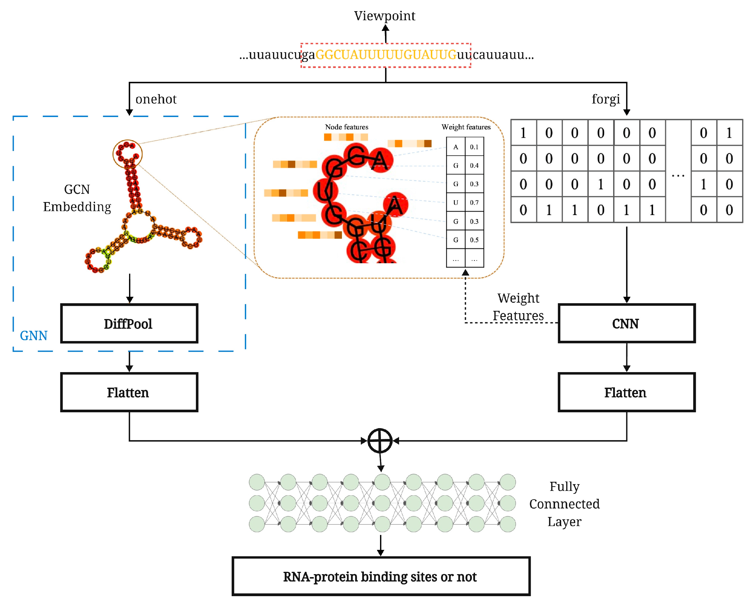
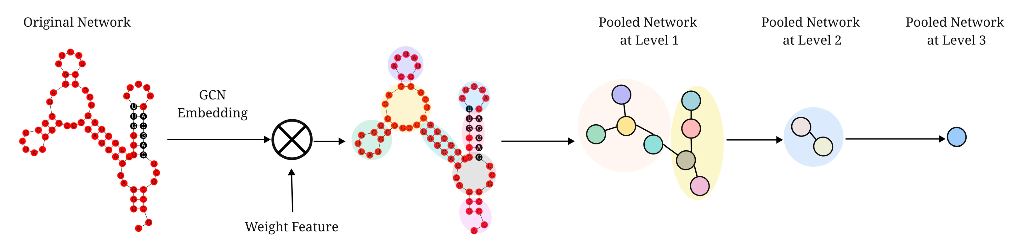
• HPNet uses DiffPool, a hierarchical pooling network, to discover hierarchical features of RNA secondary structure. It divides the substructures of the secondary structure into the same cluster and learns more meaningful graph-level embeddings;
• HPNet recognizes binding sequences and automatically extracts binding motifs using the CNN and DiffPool. It can determine whether binding sites exist and capture binding motifs without domain knowledge. The area under the curve (AUC) for HPNet was found to be significantly better than the state-of-the-art prediction method;
• A context-average debiasing method is proposed. In response to the traditional debiasing method of replacing clip sites with random nucleotides, this paper proposes a debiasing method of replacing clip sites with average-context features of clip sites.

2. Materials and Methods

2.1. Datasets and Data Processing

We research evaluated HPNet against a benchmark dataset called RBP-24, which contains 24 sub-datasets for 21 RBPs. In this dataset, 23 sub-datasets were derived from doRiNA [34], and 1 sub-dataset was derived from crosslinking immunoprecipitation (HITS-CLIP) experiments [35]. The doRiNA experiments employed photoactivated ribonucleoside-enhanced crosslinking and immunoprecipitation (PAR-CLIP) to determine binding sites. For each sub-dataset, positive samples were determined using CLIP experiments. Each positive sample had a viewpoint region of 12–75 nucleotides, the binding region determined in biological experiments. Multiple nucleotides were extended to both sides, with the viewpoint as the center, to provide more associated information from the context of the viewpoint. Negative samples were obtained by modifying positive samples when there was no supporting evidence for binding sites. In the original RBP-24 dataset, each sub-dataset consists of training and test sets. In this research, 20% of the training set was randomly selected as the validation set and 80% as the training set. Except for ALKBH5 and C7ORF85, each sub-dataset contained 500 positive and 500 negative samples for the test dataset. The details for the original RBP-24 dataset are shown in Supplementary Table S1.

2.2. Sequence Coding

“A”, “G”, “C”, and “U” are nucleotides in RNA sequences. To capture RNA sequence features, nucleotides were represented using one-hot encoding. To ensure that the inputs to the CNN had the same lengths, “N” was used to pad all sequences to the longest length, which was used as the standard in this experiment. Given an RNA sequence containing n nucleotides and a detector with a length of m, the one-hot encoding rules for the sequence were as follows.

$${\mathrm{M}}_{\mathrm{i},\mathrm{j}}=\left\{\begin{array}{l}0.25\mathrm{if}{\mathrm{s}}_{\mathrm{i}-\mathrm{m}+1}=\mathrm{N}\mathrm{o}\mathrm{r}\mathrm{i}<\mathrm{m}\mathrm{or}\mathrm{i}>n-m\\ 1\mathrm{if}{\mathrm{s}}_{\mathrm{i}-\mathrm{m}+1}\mathrm{i}\mathrm{s}\left(\mathrm{A},\mathrm{C},\mathrm{G},\mathrm{U}\right)\\ 0\mathrm{o}\mathrm{t}\mathrm{h}\mathrm{e}\mathrm{r}\mathrm{w}\mathrm{i}\mathrm{s}\mathrm{e}\end{array}\right.$$

(1)

where i represents the nucleotide position, j represents the nucleotide category, and the positions filled with “N” are expressed as a mean value of 0.25.

2.3. Secondary Structure Coding

To extract the features of RNA secondary structure, we used a library called forgi [36] to operate RNA sequences. It is a tool for converting RNA sequences into graph structures. The RNA sequences forming the most likely substructures were predicted based on minimum free energy. The resulting secondary substructures were classified as stem (S), hairpin loop (H), interior loop (I), multiloop (M), fiveprime (F), and threeprime (T) substructures, as shown in

Table 1. Abbreviations, descriptions, and common graphic representations of the six RNA secondary structure types.

Structure (Abbreviation)	Description	Graphical Representation
Stem (S)	Consecutive nucleotide-paired regions
Hairpin loop (H)	An unpaired loop structure formed by the nucleotide strings vacated between the two nucleotide strings forming the stem region
Interior loop (I)	The internal loop can contain unpaired nucleotides on either or both strands, flanked by stems
Multiloop (M)	The single-stranded region between two stems
Fiveprime (F)	The unpaired nucleotides at the 5′ end of a molecule/chain	/
Threeprime (T)	The unpaired nucleotides at the 3′ end of a molecule/chain	/

. The results were represented using one-hot encoding as the input feature matrix of the nodes. Given a sequence S, the structure encoding $\mathrm{Str}=\left({\mathrm{str}}_1,{\mathrm{str}}_2,\dots ,{\mathrm{str}}_{\mathrm{n}}\right)$ can be obtained, and the encoding rules for the substructures are as follows:

$${\mathrm{SS}}_{\mathrm{i},\mathrm{j}}=\left\{\begin{array}{l}0.16\mathrm{i}\mathrm{f}{\mathrm{str}}_{\mathrm{i}-\mathrm{m}+1}=\mathrm{N}\mathrm{o}\mathrm{r}\mathrm{i}<\mathrm{m}\mathrm{o}\mathrm{r}\mathrm{i}>n-m\\ 1\mathrm{i}\mathrm{f}{\mathrm{str}}_{\mathrm{i}-\mathrm{k}+1}is\left(\mathrm{f},\mathrm{t},\mathrm{s},\mathrm{i},\mathrm{m},\mathrm{h}\right)\\ 0\mathrm{o}\mathrm{t}\mathrm{h}\mathrm{e}\mathrm{r}\mathrm{w}\mathrm{i}\mathrm{s}\mathrm{e}\end{array}\right.$$

(2)

where i indicates the position of the substructure in the sequence, j indicates the category of the substructure, and the position filled with “N” is indicated by 0.16.

According to the forgi extracted results, some substructures may have a link between two nucleotides, but others may not. Therefore, to capture folding uncertainty and consider all the possibilities for RNA secondary structures, we adopted the RNAplfold [37] method to calculate the probability adjacency matrix for NA secondary structures.

2.4. HPNet Architecture

This research proposes a hierarchical pooling graph neural network method based on a CNN [38] and DiffPool [39]. The architecture is displayed in Figure 1. Initially, the original RNA sequences in the dataset were represented using one-hot encoding and RNA secondary structure graph representations, respectively. Then, both types of data were processed independently. A two-layer CNN was used to discover sequence features within the one-hot encoding matrix, while DiffPool was employed to extract graph representations of the RNA secondary structures. In the initial DiffPool layer, global information was learned using a GCN. Since the nodes in the graph structures corresponded to the nucleotides in the sequences, the features extracted by the same nucleotide in different models could be shared. The results of the first layer of the CNN could be expressed as weight features, representing each nucleotide’s importance in the RNA sequences. Combining the weight features with the features of each node in the graph structures highlighted the nucleotide nodes with high importance in the secondary structures, facilitating better feature extraction of the RNA secondary structures. Finally, the DiffPool and CNN results were connected and fed to the fully connected layers for prediction. The model outputs predicted labels representing the presence or absence of a binding site in the RNA sequences.

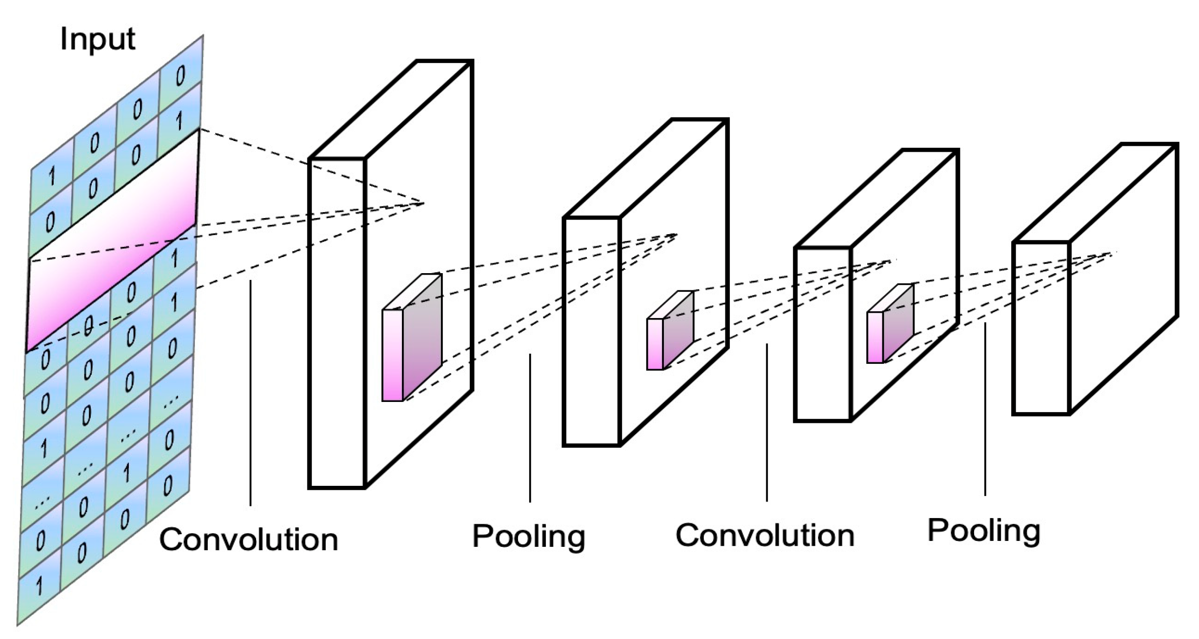
2.5. The Convolutional Neural Network in HPNet

CNNs are artificial neural networks that have been applied in many fields. Typically, a CNN consists of three layers, as shown in Figure 2: the convolutional layer, the pooling layer, and the fully connected layer. The function of the convolutional layer is to automatically extract features from the input using filters. A single convolutional layer may have poor feature extraction capabilities, while increasing the number of convolutional layers can make it possible to extract more complex features. The pooling layers mainly sample the features learned in the convolutional layers to emphasize the most critical features and prevent overfitting. The CNN adjusts the weight parameters in the model backward using gradient descent and improves its accuracy through iterative training.

The CNN’s input in this experiment was the RNA sequences’ one-hot encoding matrix. The filters moved over the input matrix with a particular step size to perform the dot product operation. Padding had to be added to the input matrix to ensure that the output matrix was the same size as the input matrix during the convolution operation. Given an input matrix $\mathrm{M}\in {ℝ}^{\mathrm{h}\times \mathrm{w}}$ and a filter $\mathrm{F}\in {ℝ}^{\mathrm{n}\times \mathrm{m}}$, the output matrix has a size of $\mathrm{X}\in {ℝ}^{\left(\mathrm{h}-\mathrm{n}+1\right)\times \left(\mathrm{w}-\mathrm{m}+1\right)}$.

The activation function is essential for a CNN to learn nonlinear features. Therefore, this research employed the rectified linear unit (ReLU) activation function, defined as follows:

$$\mathrm{ReLU}\left(\mathrm{x}\right)=\left\{\begin{array}{l}0\mathrm{i}\mathrm{f}\mathrm{x}<0\\ \mathrm{x}\mathrm{o}\mathrm{t}\mathrm{h}\mathrm{e}\mathrm{r}\mathrm{w}\mathrm{i}\mathrm{s}\mathrm{e}\end{array}\right.$$

(3)

Then, the output of the convolutional layer was fed into the pooling layer and filtered using a pooling operation to highlight the most critical features and prevent overfitting. There are two popular pooling techniques: max pooling, which selects the most significant value in the region to represent the area; and mean pooling, which determines the mean value for the part to serve as a representation. A sensible pooling operation can reduce the numbers of features and neurons and the computational burden. However, an oversampling area may result in information loss and a sharp feature reduction. In this experiment, mean pooling was used.

Finally, the high-level features obtained from pooling were flattened and fed into the fully connected layer for prediction.

2.6. DiffPool in HPNet

Various tools can be used to produce graphical representations of RNA secondary structures. Previous studies have employed CNNs or GNNs to aggregate the entire graph information directly, but they ignored the complex hierarchical relationships that may exist between each node. Therefore, this research employed DiffPool for the learning of RNA secondary structure information. DiffPool is a differentiable and end-to-end multilayer GNN model. As shown in Figure 3, in the first layer, structurally adjacent nucleotides within the same double-stranded stem or unpaired loop region were clustered into a single node in the coarsened graph of the next layer. Information extraction and node aggregation were then performed in each layer to produce a coarsening graph for the next layer. By aggregating the multilayer network, a node was obtained that represented the entire graph structure.

The layer l network in this experiment can be expressed as follows:

$${\mathrm{Z}}^{\left(\mathrm{l}\right)}=\mathrm{GNN}\left({\mathrm{A}}^{\left(\mathrm{l}\right)},{\mathrm{X}}^{\left(\mathrm{l}\right)}\right)$$

(4)

$${\mathrm{A}}^{\left(\mathrm{l}+1\right)},{\mathrm{X}}^{\left(\mathrm{l}+1\right)}=\mathrm{DiffPool}\left({\mathrm{A}}^{\left(\mathrm{l}\right)},{\mathrm{Z}}^{\left(\mathrm{l}\right)}\right)$$

(5)

where A is the predicted adjacency matrix and $\mathrm{A}\in {ℝ}^{\mathrm{n}\times \mathrm{n}}$, X is the input matrix and $\mathrm{X}\in {ℝ}^{\mathrm{n}\times \mathrm{d}}$, and Z represents the features learned by the GNN in the graph and $\mathrm{Z}\in {ℝ}^{\mathrm{n}\times \mathrm{d}}$.

DiffPool generally consists of two operations. The first employs two GNNs to extract features and learn the distribution of the node weight matrix, respectively. The distribution of nodes in the next layer is determined according to the node weight matrix. The two GNNs use similar methods.

$${\mathrm{Z}}^{\left(\mathrm{l}\right)}={\mathrm{GNN}}_{\mathrm{l},\mathrm{embed}}\left({\mathrm{A}}^{\left(\mathrm{l}\right)},{\mathrm{X}}^{\left(\mathrm{l}\right)}\right)$$

(6)

$${\mathrm{S}}^{\left(\mathrm{l}\right)}=\mathrm{softmax}\left({\mathrm{GNN}}_{\mathrm{l},\mathrm{pool}}\left({\mathrm{A}}^{\left(\mathrm{l}\right)},{\mathrm{X}}^{\left(\mathrm{l}\right)}\right)\right)$$

(7)

The second operation is the aggregation of nodes according to the node weight matrix, which can be written mathematically as follows:

$${\mathrm{X}}^{\left(\mathrm{l}+1\right)}={\mathrm{S}}^{{\left(\mathrm{l}\right)}^{\mathrm{T}}}{\mathrm{Z}}^{\left(\mathrm{l}\right)}\in {ℝ}^{{\mathrm{n}}_{\mathrm{l}+1}\times \mathrm{d}}$$

(8)

$${\mathrm{A}}^{\left(\mathrm{l}+1\right)}={\mathrm{S}}^{{\left(\mathrm{l}\right)}^{\mathrm{T}}}{\mathrm{A}}^{\left(\mathrm{l}\right)}{\mathrm{S}}^{\left(\mathrm{l}\right)}\in {ℝ}^{{\mathrm{n}}_{\mathrm{l}+1}\times {\mathrm{n}}_{\mathrm{l}+1}}$$

(9)

This experiment used a GCN for the initial GNN layer, while GraphSAGE [40] was used for the remaining GNN. The information transfer equation for the GCN algorithm can be expressed as follows.

$${\mathrm{H}}^{\left(\mathrm{k}\right)}=\mathrm{M}\left(\mathrm{A},{\mathrm{H}}^{\left(\mathrm{k}-1\right)};{\mathrm{W}}^{\left(\mathrm{k}\right)}\right)=\mathrm{ReLU}\left({\tilde{\mathrm{D}}}^{-\frac{1}{2}}{\tilde{\mathrm{A}}\tilde{\mathrm{D}}}^{-\frac{1}{2}}{\mathrm{H}}^{\left(\mathrm{k}-1\right)}{\mathrm{W}}^{\left(\mathrm{k}-1\right)}\right)$$

(10)

where H denotes the input matrix and k denotes the k-th layer network.

DiffPool is a non-convex optimization model. Two regularization terms are added to the model to prevent the model from falling into the local minimum, which can be written as follows.

$${\mathrm{L}}_{\mathrm{LP}}={\Vert {\mathrm{A}}^{\left(\mathrm{l}\right)},{\mathrm{S}}^{\left(\mathrm{l}\right)}{\mathrm{S}}^{{\left(\mathrm{l}\right)}^{\mathrm{T}}}\Vert }_{\mathrm{F}}$$

(11)

$${\mathrm{L}}_{\mathrm{E}}=\frac{1}{\mathrm{n}}{{\displaystyle \sum }}_{\mathrm{i}=1}^{\mathrm{n}}\mathrm{H}\left({\mathrm{S}}_{\mathrm{i}}\right)$$

(12)

The first regularization term can assist the link in predicting the target. It minimizes ${\mathrm{L}}_{\mathrm{LP}}$ and continuously corrects ${\mathrm{S}}^{\left(\mathrm{l}\right)}$, ensuring that two highly similar nodes are mapped to the same coarsening node. The second regularization term reduces the uncertainty of the mapping distribution to ensure that each node is assigned to a coarsening node.

After each DiffPool operation, the number of graph nodes decreases until a single node is obtained that aggregates the information for the entire graph.

2.7. Fully Connected Layer and Loss Function

The fully connected layer was designed to mimic the neural architecture of the human brain, where each node in the layer is connected to all the nodes in the following layer. Classification based on the features previously extracted by the CNN and DiffPool was the fundamental goal of the fully connected layer. It took these features as inputs and used three fully connected layers to make a prediction.

The loss function was used to measure the percentage difference between the predicted and actual values to optimize the model. When the loss values did not meet the requirements, backpropagation was employed to adjust the parameters to minimize the loss and improve the stability of the model. The binary cross-entropy loss function was implemented in this experiment to discover model parameters without introducing gradient dissipation.

$$\mathrm{L}\left(\mathrm{w}\right)=-{\displaystyle \sum }_{\mathrm{i}=1}^{\mathrm{n}}{\mathrm{y}}_{\mathrm{i}}\log \left(\widehat{{\mathrm{y}}_{\mathrm{i}}}\right)+\left(1-{\mathrm{y}}_{\mathrm{i}}\right)\log \left(1-\widehat{{\mathrm{y}}_{\mathrm{i}}}\right)$$

(13)

where the actual label is $y_i$ and the predicted label is $\widehat{{\mathrm{y}}_{\mathrm{i}}}$.

2.8. Debiasing Data

In biological experiments, RNA cleavage enzymes are commonly utilized to isolate specific RNA sequences. The method often results in many positive samples with identical cleavage sites, which means that the nucleotides at the beginning and end of the RNA viewpoint fragments are identical. In the positive samples, the viewpoints usually begin with “G” and end with “G”. However, machine-learning models tend to emphasize RNA fragment boundaries more during feature extraction, leading to biased results. Therefore, removing the bias in the data can ensure the prediction results’ authenticity. RPI-Net suggests solving the problem by replacing boundary nucleotides with random nucleotides. However, we found that this method can lead to the loss of information in the combined sequence and increase the uncertainty of the prediction results. Notably, the sequence context has a vital role in selecting binding sites. Therefore, this research proposes a debiasing method that incorporates boundary contexts. In other words, the areas three nucleotides ahead and behind of the central nucleotide served as the context. The mean values of the context features replaced the feature of the central nucleotide. This method involved replacing the nucleotides in a window of size 3 centered at the “G” preceding the viewpoint and in a window of size 3 centered at the end of the viewpoint. It could maximize the integrity of the combined information. Given an RNA sequence S, the feature calculation method for its boundary nucleotides is as follows.

$${\mathrm{F}}_{\mathrm{i}}=\frac{1}{6}{{\displaystyle \sum }}_{\mathrm{j}=-3}^3{\mathrm{F}}_{\mathrm{i}+\mathrm{j}}$$

(14)

where F represents the feature matrix of the RNA sequences, i represents the position of the nucleotide, and j represents the position of the context of nucleotide i.

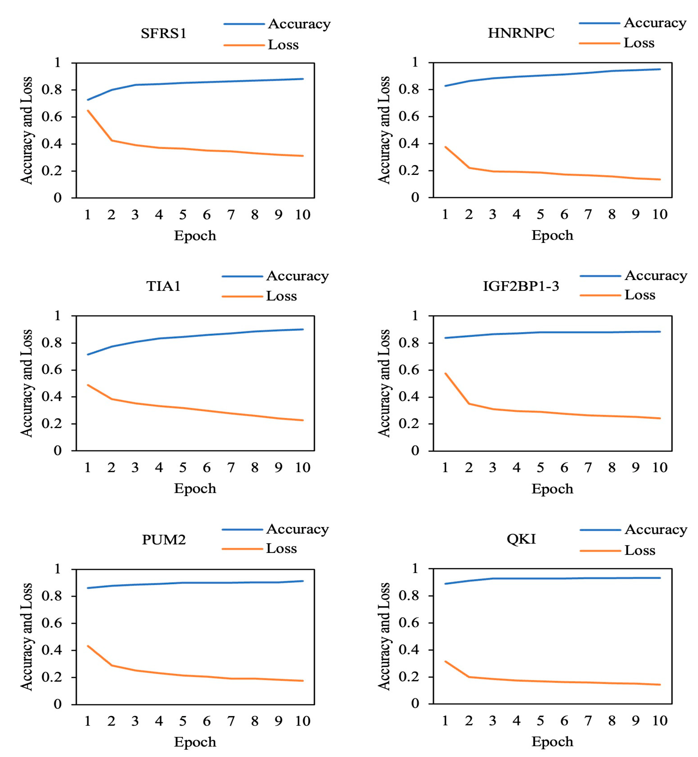
2.9. Parameter Optimization

We used the Pytorch framework in Ubuntu to create the model and accelerated using GPU. The Adam algorithm was employed for optimization during model training, and the maximum number of model iterations was set to 50. Due to the massive size of the training set, the computational performance of the model would have been reduced if sub-datasets were traversed directly during each iteration. Thus, the mini-batch algorithm was introduced into the experiment. It undertakes calculations while making adjustments by using small samples for calculation and by making several gradient descents in a traversal. The calculation efficiency is thus increased while the time complexity is decreased. Typically, a power of 2 between 64 and 512 is chosen as the mini-batch size. Mini-batch sizes of 128 were used in the experiment because they struck a balance between speed and precision. Furthermore, a GCN was used to learn the graph structure globally, which is necessary when learning the hierarchical features of a secondary structure. The dropout approach was implemented during training to prevent local optimization of model parameters. By randomly discarding some neurons, the random correction of the extracted features and the avoidance of overfitting were achieved. We used the AUC as the model evaluation metric. The AUC evaluates the classification ability of a model; here, the ability of HPNet to correctly predict the presence of binding sites in RNA. In general, larger AUC values are better.

3. Results

3.1. Baseline

Numerous deep-learning methods have been applied to predict RNA-binding sites. HPNet was evaluated in this experiment and compared to the following methods:

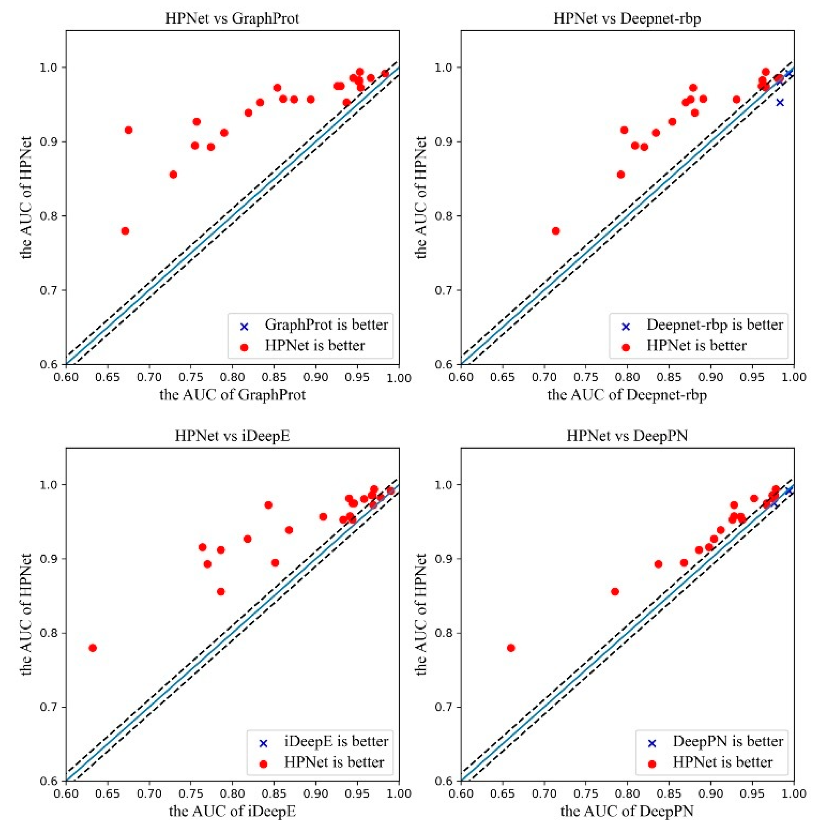
• GraphProt: This method uses a hypergraph to describe the RNA secondary structure fully and uses a graph kernel approach to extract features from the hypergraph. The model is then trained through machine learning based on the features to predict RNA-binding sites;
• Deepnet-rbp [41]: This method added the RNA tertiary structure to the prediction model for the first time. It involves constructing a framework containing the RNA sequence, secondary structure, and tertiary structure, which represent the specificities of the RBP-binding sites in three dimensions, respectively;
• iDeppE: This method uses two CNNs to learn global and local RNA sequence features. For the global CNN, an entire sequence is padded to the same length and used directly as the input. For the local CNN, an RNA sequence is split into multiple overlapping fixed-length subsequences, and each sub-sequence is used as a separate signal channel of the full-length sequence. The two CNNs are trained independently and then combined for prediction;
• RPI-Net: This method introduces GCN and LSTM deep-learning models. The graphical representation of RNA secondary structure can be effectively learned using the GCN and message passing takes place through the LSTM. The learned graphical features are then inputted into the Bi-LSTM to learn the global embedding. An end-to-end learning method is implemented;
• DeepPN: This method consists of a CNN and a GCN, a parallel learning network. The CNN and GCN are used to learn sequence features from different perspectives to compensate for the lack of features.

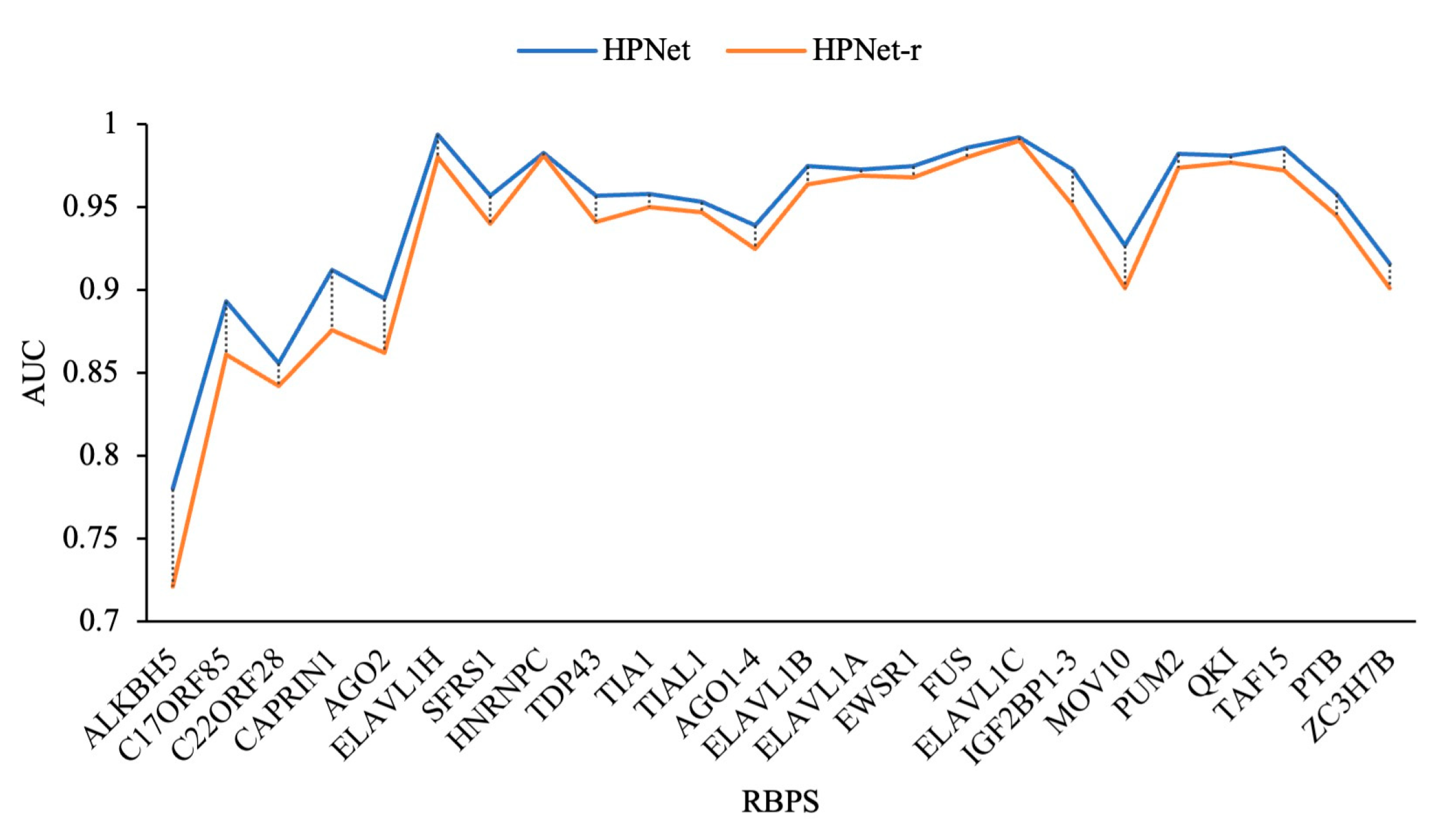
3.2. Prediction Results for the Original Dataset

As shown in

Table 2. Performance of HPNet and baseline methods with RBP-24 dataset.

RBPs	GraphProt	Deepnet-rbp	iDeepE	DeepPN	HPNet
ALKBH5	0.68	0.714	0.758	0.66	0.78
C17ORF85	0.800	0.820	0.830	0.837	0.893
C22ORF28	0.751	0.792	0.837	0.785	0.856
CAPRIN1	0.855	0.834	0.893	0.886	0.912
AGO2	0.765	0.809	0.884	0.868	0.895
ELAVL1H	0.955	0.966	0.979	0.978	0.994
SFRS1	0.898	0.931	0.946	0.936	0.957
HNRNPC	0.952	0.962	0.976	0.977	0.983
TDP43	0.874	0.876	0.945	0.936	0.957
TIA1	0.861	0.891	0.937	0.928	0.958
TIAL1	0.833	0.870	0.934	0.926	0.953
AGO1-4	0.895	0.881	0.915	0.912	0.939
ELAVL1B	0.935	0.961	0.971	0.976	0.975
ELAVL1A	0.959	0.966	0.964	0.967	0.973
EWSR1	0.935	0.966	0.969	0.954	0.975
FUS	0.968	0.980	0.985	0.977	0.986
ELAVL1C	0.991	0.994	0.988	0.994	0.992
IGF2BP1-3	0.889	0.879	0.947	0.928	0.973
MOV10	0.863	0.854	0.916	0.904	0.927
PUM2	0.954	0.971	0.967	0.952	0.982
QKI	0.957	0.983	0.970	0.975	0.981
TAF15	0.970	0.983	0.976	0.974	0.986
PTB	0.937	0.983	0.944	0.938	0.958
ZC3H7B	0.820	0.796	0.907	0.898	0.916
Mean	0.887	0.902	0.931	0.919	0.945

, HPNet achieved the best mean AUC of 0.945 with the RBP-24 dataset, 6.5% higher than GraphProt, 4.8% higher than Deepnet-rbp, 1.5% higher than iDeepE, and 2.8% higher than DeepPN. Moreover, HPNet achieved the best AUCs with 21 sub-datasets, with AUCs of 0.95 or higher with 16 sub-datasets. Among these baseline models, iDeepE and DeepPN only use RNA sequence features for model training, limiting their ability to learn RNA structure information and decreasing prediction accuracy. GraphProt adds RNA secondary structure information to the model, expressed as a graph structure. However, GraphProt uses machine-learning methods to train the model, which depend on pre-processing features and may cause problems, such as feature loss. The tertiary structure of RNA is predicted based on the secondary structure. Deepnet-rbp incorporates the tertiary structure into the model, and all three dimensions indicate binding specificity. However, the prediction of RNA tertiary structure is challenging and uncertain, which may also lead to feature loss and decreased accuracy.

HPNet introduces the concept of hierarchical pooling in its utilization of secondary structures. It has been shown experimentally that RNA hierarchical features play an essential role in RBP–RNA interaction. For example, for the ZC3H7B protein, HPNet achieved a 1.9% improvement over iDeepE and a 13% improvement over Deepnet-rbp. Notably, HPNet performed better with RBPs with smaller training sets, such as ALKBH5, which has 2410 training samples, and C17ORF85, which has 3709 training samples.

Figure 4 depicts the results of a statistical comparison of the four methods and HPNet. If the AUC of HPNet was higher than that of the baseline method with the same sub-dataset, it is marked with “.”. Otherwise, it is marked with “x”. Each dotted line in the figure represents a difference of 1%, and the p-value represents the significance test level. Generally, two methods are significantly different when the p-value is less than or equal to 0.05. A p-value of less than 0.001 indicates a highly significant difference. Figure 4 shows that the p-values for all four experiments were significantly lower than 0.001, demonstrating that HPNet is markedly different from the other four methods.

In the experiment, the model automatically stopped training when the loss of the test sets was lower than 0.1 or the number of epochs reached 50. Figure 5 shows the training process for six sub-datasets. When the number of epochs was set to 10, the accuracies for the test sets exceeded 0.8. The accuracy gradually improved as the loss decreased until the stopping criterion was met.

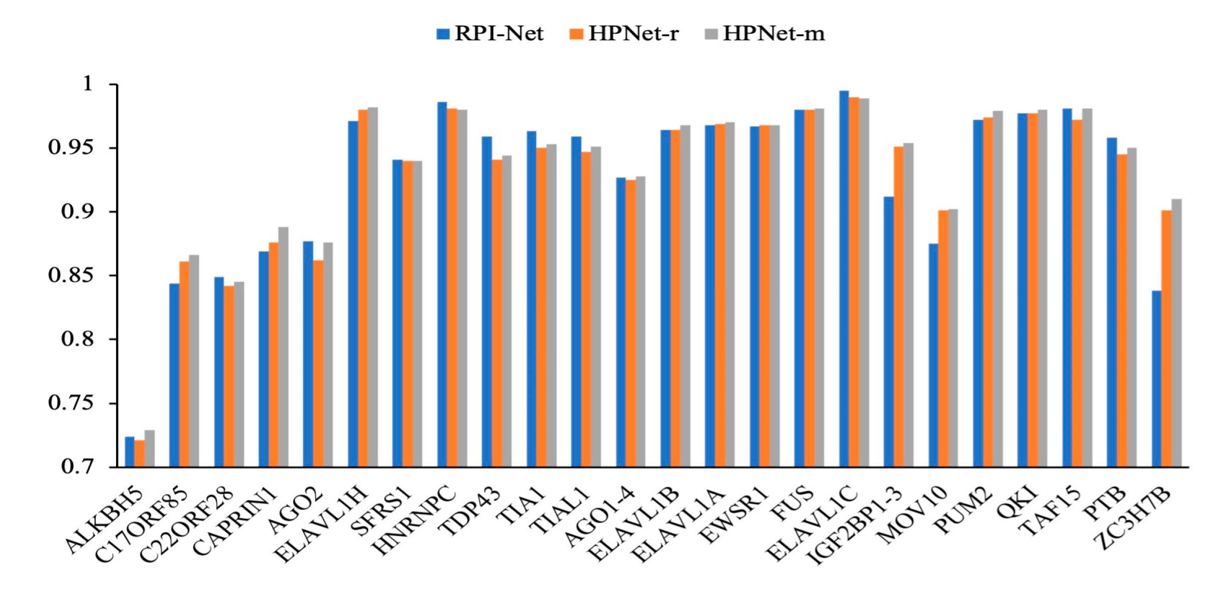
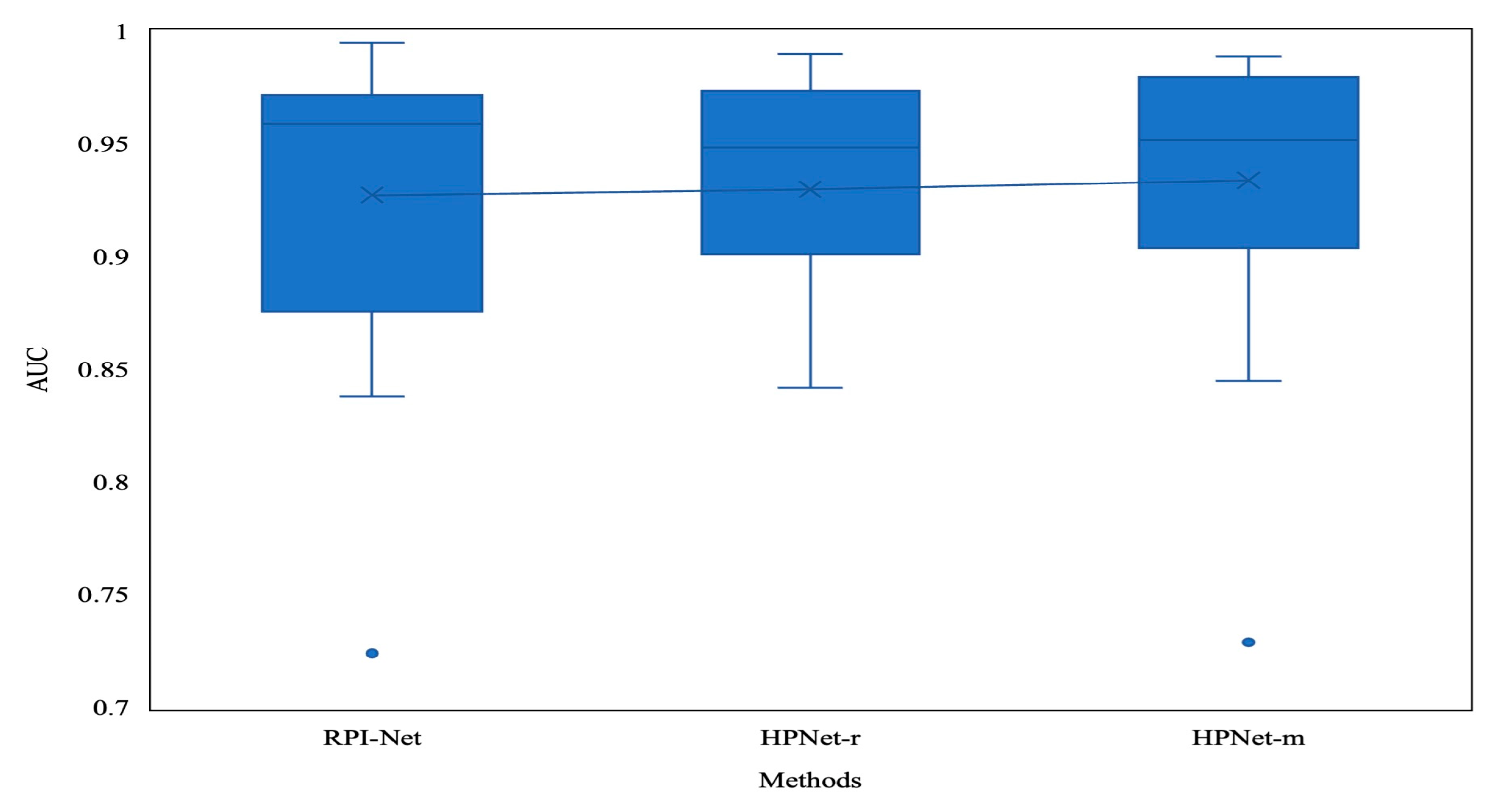
3.3. Prediction Results for the Debiased Datasets

To evaluate the effectiveness of the proposed debiasing method, both the context-average debiasing method and the RPI-Net random debiasing method were evaluated in this experiment. HPNet-r uses the random debiasing method, while HPNet-m uses the context-average debiasing method. The experimental results are shown in

Table 3. Mean AUCs of three debiasing methods.

Method	Mean AUC
RPI-Net	0.927
HPNet-r	0.930
HPNet-m	0.933

; the mean AUC for RPI-Net was 0.927, the mean AUC for HPNet-r was 0.930, and the mean AUC for HPNet-m was 0.933. HPNet-r performed better than RPI-Net, and HPNet-m performed better than HPNet-r. Although RPI-Net automatically extracts features from secondary structures and sequences through a GCN and LSTM and has improved prediction accuracy, it ignores the hierarchical features of secondary structures, resulting in a slightly lower accuracy than HPNet-r and HPNet-m.

Figure 6 shows the performance results for the three methods with debiased data. It can be observed that the performance of HPNet-r was better than that of RPI-Net with some proteins, with the most significant improvement observed with the protein ZC3H7B at 7.5%. The box diagram in Figure 7 demonstrates that the median for HPNet-r was smaller than for RPI-Net, but the range for HPNet-r was smaller than for RPI-Net, indicating that HPNet had better stability. The median and average values for HPNet-m were more significant than those for HPNet-r, confirming the effectiveness of the context-average debiasing method proposed in this research. It can be seen from Figure 8 that when the data were debiased, the AUCs of most proteins decreased. The AUCs of several proteins, such as ALKBH5, CAPRIN1, and MOV10, decreased significantly. The reduced performance of ALKBH5 can be attributed to the small dataset, while the deviations in the dataset for CAPRIN1 and MOV10, which were obtained in the PAR-CLIP experiment, were relatively large.

3.4. Motif Visualizations

In this research, binding motifs representing binding preferences were automatically extracted according to the parameters and other information in HPNet. Based on the results of a biological study, a database of RBP motifs and specificities has been constructed named the RNA Inferred Sequence Binding Protein Catalog (CISBP-RNA) [42]. Therefore, the patterns retrieved by HPNet can be compared with the motifs in CISBP-RNA. TOMTOM [43] can fulfill this function. It rates the similarity between the input motifs and the pre-existing database of known motifs and selects the p-value as the measure.

In this experiment, the first-layer output of the GCN represented the importance of the nucleotide nodes. The weights output by the first layer of the CNN represented the importance of the nucleotides in the sequence. The mean value for the node importance and sequence importance for each nucleotide was calculated as the nucleotide-binding affinity and expanded into 7-mer motifs centered on the most significant 5% of nucleotides. Then, the RCK technique was utilized to convert the binding nucleotide sequences into PWM based on the selected nucleotides. We used TOMTOM to visualize and compare experimentally generated motifs.

Table 4. Comparison of motifs extracted by HPNet (bottom) and motifs in the CISBP-RNA database (top).

RBPs	Motifs	RBPs	Motifs	RBPs	Motifs
HNRNPC	p-value: 3.22 × 10−5	SRSF1	p-value: 3.58 × 10−3	TIA1	p-value: 5.70 × 10−4
PUM2	p-value: 9.02 × 10−4	QKI	p-value: 1.41 × 10−4	IGF2BP123	p-value: 9.66 × 10−5

displays the RBP-binding motifs extracted by HPNet and the motifs in the CISBP-RNA database. It also shows the “U” enrichment in the binding motif of TIA1 and HNRNPC proteins. The results of TOMTOM were consistent with the motifs previously found in CISBP-RNA, with p-values of 0.00046 and 0.00017, respectively. The binding motif of the SFRS1 protein was rich in the segment of “GAGGA”, which was the same as a result in the CISBP-RNA database. According to the CISBP-RNA database, the “UGCA” region was highly typical in the binding motif of the PUM2 protein. The binding motif of the protein QKI contained a “CUAA” fragment. However, the outcomes for the IGF2BP1-3 protein need to be made clearer.

However, the CISBP-RNA database only contains known experimental RBP binding motifs. Several RBPs have binding motifs that still need to be verified. Therefore, we employed Multiple EM for Motive Elicitation (MEME) [44] to develop the models of untested binding motifs, as given in

Table 5. Binding motifs extracted by the HPNet model but not in the database.

RBPs	Motifs	RBPs	Motifs	RBPs	Motifs	RBPs	Motifs
ALKBH5		C17ORF85		C22ORF28		CAPRIN1
AGO2		TDP43		TAF15		TIAL1
AGO1234		ELAVL1A		ELAVL1B		ELAVL1C
ELAVL1H		EWSR1		FUS		ZC3H7B
MOV10		PTB

, which also compares the results with relevant previous findings. Table 5 demonstrates that the ELAVL1 protein and its related proteins have a high affinity for “U”-rich motifs, consistent with the biological experiment results in [45]. The binding motif of the TIAL1 protein and TIA1 protein is rich in “UU”, consistent with the results from [46]. In addition, the binding motifs of FUS, TAF15, and EWSR1 are rich in “AU”, while PTB is rich in “UC”. The character’s height indicates each position’s information retention degree (bit) at that point in the illustration.

4. Discussion

Despite HPNet’s significant performance gains, it can still be improved in many ways. First, HPNet uses a CNN to study sequence features. However, all sequences must be the same length, and the padding values are replaced by mean values, which can introduce bias in the learning results and require additional storage space. The CCNN approach [47] described by Romero et al. can be utilized to address this issue. It employs a universal CNN that works with inputs of arbitrary length. Second, HPNet uses DiffPool to learn RNA secondary structure hierarchical information. However, dense graphs can be generated after pooling, which can increase the complexity of the model and reduce the computational efficiency. To overcome this problem, the self-attention approach can be used to simplify the network and speed up computation by eliminating unneeded nodes. Finally, while HPNet uses a deep-learning network for prediction, the details of how it arrives at its conclusions are hidden from view. Therefore, it is crucial to investigate the interpretability of the deep learning, as it could shed light on the RBP–RNA binding process.

5. Conclusions

This paper proposes a deep-learning method based on hierarchical pooling called HPNet for the prediction of RBP–-RNA binding sites. Additionally, a debiasing method targeting clip boundaries is also proposed. First, a CNN is used to learn RNA sequence features. The first-layer results are considered weights for the nucleotides, which can guide DiffPool in learning the hierarchical features of the secondary structure. DiffPool then clusters similar nodes in each layer into the same cluster. Finally, the sequence features and the hierarchical features of the secondary structure are connected for prediction. The method was trained and evaluated with the original and debiased RBP-24 datasets. It could be concluded that: (1) HPNet could automatically identify binding sites and extract binding preferences, and its AUC outperformed the state-of-the-art methods; (2) the hierarchical features of the secondary structure play an essential role in RBP–RNA binding; (3) the context-average debiasing method is effective.

References

1. McHugh, C.A.; Russell, P.; Guttman, M. Methods for Comprehensive Experimental Identification of RNA-Protein Interactions. Genome Biol. 2014, 15, 203. [Google Scholar] [CrossRef] [PubMed] [Green Version]
2. Breaker, R.R.; Joyce, G.F. The Expanding View of RNA and DNA Function. Chem. Biol. 2014, 21, 1059–1065. [Google Scholar] [CrossRef] [PubMed] [Green Version]
3. Dominguez, D.; Freese, P.; Alexis, M.S.; Su, A.; Hochman, M.; Palden, T.; Bazile, C.; Lambert, N.J.; Van Nostrand, E.L.; Pratt, G.A.; et al. Sequence, Structure, and Context Preferences of Human RNA Binding Proteins. Mol. Cell 2018, 70, 854–867.e9. [Google Scholar] [CrossRef] [PubMed] [Green Version]
4. Achsel, T.; Bagni, C. Cooperativity in RNA–Protein Interactions: The Complex Is More than the Sum of Its Partners. Curr. Opin. Neurobiol. 2016, 39, 146–151. [Google Scholar] [CrossRef]
5. Oliveira, C.; Faoro, H.; Alves, L.R.; Goldenberg, S. RNA-Binding Proteins and Their Role in the Regulation of Gene Expression in Trypanosoma Cruzi and Saccharomyces Cerevisiae. Genet. Mol. Biol. 2017, 40, 22–30. [Google Scholar] [CrossRef] [Green Version]
6. Re, A.; Joshi, T.; Kulberkyte, E.; Morris, Q.; Workman, C.T. RNA-Protein Interactions: An Overview. Methods Mol. Biol. 2014, 1097, 491–521. [Google Scholar] [CrossRef]
7. Ramanathan, M.; Porter, D.F.; Khavari, P.A. Methods to Study RNA–Protein Interactions. Nat. Methods 2019, 16, 225–234. [Google Scholar] [CrossRef]
8. Cozzolino, F.; Iacobucci, I.; Monaco, V.; Monti, M. Protein–DNA/RNA Interactions: An Overview of Investigation Methods in the -Omics Era. J. Proteome Res. 2021, 20, 3018–3030. [Google Scholar] [CrossRef]
9. Corley, M.; Burns, M.C.; Yeo, G.W. How RNA-Binding Proteins Interact with RNA: Molecules and Mechanisms. Mol. Cell 2020, 78, 9–29. [Google Scholar] [CrossRef]
10. Xue, Y.; Zhou, Y.; Wu, T.; Zhu, T.; Ji, X.; Kwon, Y.-S.; Zhang, C.; Yeo, G.; Black, D.L.; Sun, H.; et al. Genome-Wide Analysis of PTB-RNA Interactions Reveals a Strategy Used by the General Splicing Repressor to Modulate Exon Inclusion or Skipping. Mol. Cell 2009, 36, 996–1006. [Google Scholar] [CrossRef] [Green Version]
11. Gebauer, F.; Schwarzl, T.; Valcárcel, J.; Hentze, M.W. RNA-Binding Proteins in Human Genetic Disease. Nat. Rev. Genet. 2021, 22, 185–198. [Google Scholar] [CrossRef]
12. Ascano, M.; Hafner, M.; Cekan, P.; Gerstberger, S.; Tuschl, T. Identification of RNA–Protein Interaction Networks Using PAR-CLIP. Wiley Interdiscip. Rev. RNA 2012, 3, 159–177. [Google Scholar] [CrossRef] [Green Version]
13. Nechay, M.; Kleiner, R.E. High-Throughput Approaches to Profile RNA-Protein Interactions. Curr. Opin. Chem. Biol. 2020, 54, 37–44. [Google Scholar] [CrossRef] [PubMed]
14. König, J.; Zarnack, K.; Luscombe, N.M.; Ule, J. Protein–RNA Interactions: New Genomic Technologies and Perspectives. Nat. Rev. Genet. 2012, 13, 77–83. [Google Scholar] [CrossRef] [PubMed]
15. Zhao, J.; Ohsumi, T.K.; Kung, J.T.; Ogawa, Y.; Grau, D.J.; Sarma, K.; Song, J.J.; Kingston, R.E.; Borowsky, M.; Lee, J.T. Genome-Wide Identification of Polycomb-Associated RNAs by RIP-Seq. Mol. Cell 2010, 40, 939–953. [Google Scholar] [CrossRef] [PubMed] [Green Version]
16. Vanegas, P.L.; Hudson, G.A.; Davis, A.R.; Kelly, S.C.; Kirkpatrick, C.C.; Znosko, B.M. RNA CoSSMos: Characterization of Secondary Structure Motifs—A Searchable Database of Secondary Structure Motifs in RNA Three-Dimensional Structures. Nucleic Acids Res. 2012, 40, D439–D444. [Google Scholar] [CrossRef] [Green Version]
17. Balcerak, A.; Trebinska-Stryjewska, A.; Konopinski, R.; Wakula, M.; Grzybowska, E.A. RNA-Protein Interactions: Disorder, Moonlighting and Junk Contribute to Eukaryotic Complexity. Open Biol. 2019, 9, 190096. [Google Scholar] [CrossRef] [PubMed] [Green Version]
18. Jolma, A.; Zhang, J.; Mondragón, E.; Morgunova, E.; Kivioja, T.; Laverty, K.U.; Yin, Y.; Zhu, F.; Bourenkov, G.; Morris, Q.; et al. Binding Specificities of Human RNA-Binding Proteins toward Structured and Linear RNA Sequences. Genome Res. 2020, 30, 962–973. [Google Scholar] [CrossRef]
19. Scarselli, F.; Gori, M.; Tsoi, A.C.; Hagenbuchner, M.; Monfardini, G. The Graph Neural Network Model. IEEE Trans. Neural Netw. 2009, 20, 61–80. [Google Scholar] [CrossRef] [Green Version]
20. Wang, Z.; Dai, Q.; Song, J.; Duan, X.; Yang, H.; Yang, Z. Predicting RBP Binding Sites of RNA With High-Order Encoding Features and CNN-BLSTM Hybrid Model. IEEE/ACM Trans. Comput. Biol. Bioinform. 2022, 19, 2409–2419. [Google Scholar] [CrossRef]
21. Macke, T.J.; Ecker, D.J.; Gutell, R.R.; Gautheret, D.; Case, D.A.; Sampath, R. RNAMotif, an RNA Secondary Structure Definition and Search Algorithm. Nucleic Acids Res. 2001, 29, 4724–4735. [Google Scholar] [CrossRef] [PubMed]
22. Chełkowska-Pauszek, A.; Kosiński, J.G.; Marciniak, K.; Wysocka, M.; Bąkowska-Żywicka, K.; Żywicki, M. The Role of RNA Secondary Structure in Regulation of Gene Expression in Bacteria. Int. J. Mol. Sci. 2021, 22, 7845. [Google Scholar] [CrossRef] [PubMed]
23. Kazan, H.; Ray, D.; Chan, E.T.; Hughes, T.R.; Morris, Q. RNAcontext: A New Method for Learning the Sequence and Structure Binding Preferences of RNA-Binding Proteins. PLoS Comput. Biol. 2010, 6, e1000832. [Google Scholar] [CrossRef] [Green Version]
24. Orenstein, Y.; Wang, Y.; Berger, B. RCK: Accurate and Efficient Inference of Sequence- and Structure-Based Protein–RNA Binding Models from RNAcompete Data. Bioinformatics 2016, 32, i351–i359. [Google Scholar] [CrossRef] [Green Version]
25. Maticzka, D.; Lange, S.J.; Costa, F.; Backofen, R. GraphProt: Modeling Binding Preferences of RNA-Binding Proteins. Genome Biol. 2014, 15, R17. [Google Scholar] [CrossRef] [Green Version]
26. Alipanahi, B.; Delong, A.; Weirauch, M.T.; Frey, B.J. Predicting the Sequence Specificities of DNA- and RNA-Binding Proteins by Deep Learning. Nat. Biotechnol. 2015, 33, 831–838. [Google Scholar] [CrossRef] [PubMed]
27. Pan, X.; Shen, H.-B. Predicting RNA-Protein Binding Sites and Motifs through Combining Local and Global Deep Convolutional Neural Networks. Bioinformatics 2018, 34, 3427–3436. [Google Scholar] [CrossRef] [Green Version]
28. Pan, X.; Rijnbeek, P.; Yan, J.; Shen, H.-B. Prediction of RNA-Protein Sequence and Structure Binding Preferences Using Deep Convolutional and Recurrent Neural Networks. BMC Genom. 2018, 19, 1–11. [Google Scholar] [CrossRef] [Green Version]
29. Deng, L.; Liu, Y.; Shi, Y.; Zhang, W.; Yang, C.; Liu, H. Deep Neural Networks for Inferring Binding Sites of RNA-Binding Proteins by Using Distributed Representations of RNA Primary Sequence and Secondary Structure. BMC Genom. 2020, 21, 866. [Google Scholar] [CrossRef]
30. Yan, J.; Zhu, M. A Review About RNA–Protein-Binding Sites Prediction Based on Deep Learning. IEEE Access 2020, 8, 150929–150944. [Google Scholar] [CrossRef]
31. Yan, Z.; Hamilton, W.L.; Blanchette, M. Graph Neural Representational Learning of RNA Secondary Structures for Predicting RNA-Protein Interactions. Bioinformatics 2020, 36, i276–i284. [Google Scholar] [CrossRef] [PubMed]
32. Zhang, S.; Tong, H.; Xu, J.; Maciejewski, R. Graph Convolutional Networks: A Comprehensive Review. Comput. Soc. Netw. 2019, 6, 11. [Google Scholar] [CrossRef] [Green Version]
33. Zhang, J.; Liu, B.; Wang, Z.; Lehnert, K.; Gahegan, M. DeepPN: A Deep Parallel Neural Network Based on Convolutional Neural Network and Graph Convolutional Network for Predicting RNA-Protein Binding Sites. BMC Bioinform. 2022, 23, 257. [Google Scholar] [CrossRef] [PubMed]
34. Anders, G.; Mackowiak, S.D.; Jens, M.; Maaskola, J.; Kuntzagk, A.; Rajewsky, N.; Landthaler, M.; Dieterich, C. DoRiNA: A Database of RNA Interactions in Post-Transcriptional Regulation. Nucleic Acids Res. 2012, 40, D180–D186. [Google Scholar] [CrossRef] [PubMed]
35. Hafner, M.; Katsantoni, M.; Köster, T.; Marks, J.; Mukherjee, J.; Staiger, D.; Ule, J.; Zavolan, M. CLIP and Complementary Methods. Nat. Rev. Methods Prim. 2021, 1, 20. [Google Scholar] [CrossRef]
36. Thiel, B.C.; Beckmann, I.K.; Kerpedjiev, P.; Hofacker, I.L. 3D Based on 2D: Calculating Helix Angles and Stacking Patterns Using Forgi 2.0, an RNA Python Library Centered on Secondary Structure Elements. F1000Research 2019, 8, 287. [Google Scholar] [CrossRef] [PubMed]
37. Bernhart, S.H.; Hofacker, I.L.; Stadler, P.F. Local RNA Base Pairing Probabilities in Large Sequences. Bioinformatics 2006, 22, 614–615. [Google Scholar] [CrossRef] [Green Version]
38. Lecun, Y.; Bottou, L.; Bengio, Y.; Haffner, P. Gradient-Based Learning Applied to Document Recognition. Proc. IEEE 1998, 86, 2278–2324. [Google Scholar] [CrossRef] [Green Version]
39. Ying, R.; You, J.; Morris, C.; Ren, X.; Hamilton, W.L.; Leskovec, J. Hierarchical Graph Representation Learning with Differentiable Pooling. In Proceedings of the 32nd International Conference on Neural Information Processing Systems, Vancouver, BC, Canada, 8–14 December 2019; Curran Associates Inc.: Red Hook, NY, USA, 2018; pp. 4805–4815. [Google Scholar]
40. Hamilton, W.L.; Ying, R.; Leskovec, J. Inductive Representation Learning on Large Graphs. In Proceedings of the 31st International Conference on Neural Information Processing Systems, Montreal, QC, Canada, 3–8 December 2018; Curran Associates Inc.: Red Hook, NY, USA, 2017; pp. 1025–1035. [Google Scholar]
41. Zhang, S.; Zhou, J.; Hu, H.; Gong, H.; Chen, L.; Cheng, C.; Zeng, J. A Deep Learning Framework for Modeling Structural Features of RNA-Binding Protein Targets. Nucleic Acids Res. 2016, 44, e32. [Google Scholar] [CrossRef] [Green Version]
42. Ray, D.; Kazan, H.; Cook, K.B.; Weirauch, M.T.; Najafabadi, H.S.; Li, X.; Gueroussov, S.; Albu, M.; Zheng, H.; Yang, A.; et al. A Compendium of RNA-Binding Motifs for Decoding Gene Regulation. Nature 2013, 499, 172–177. [Google Scholar] [CrossRef] [Green Version]
43. Tanaka, E.; Bailey, T.; Grant, C.E.; Noble, W.S.; Keich, U. Improved Similarity Scores for Comparing Motifs. Bioinformatics 2011, 27, 1603–1609. [Google Scholar] [CrossRef] [Green Version]
44. Bailey, T.L.; Elkan, C. Fitting a Mixture Model by Expectation Maximization to Discover Motifs in Biopolymers. Proc. Int. Conf. Intell. Syst. Mol. Biol. 1994, 2, 28–36. [Google Scholar]
45. Kota, S.K.; Lim, Z.W.; Kota, S.B. Elavl1 Impacts Osteogenic Differentiation and MRNA Levels of Genes Involved in ECM Organization. Front. Cell Dev. Biol. 2021, 9, 606971. [Google Scholar] [CrossRef] [PubMed]
46. Dember, L.M.; Kim, N.D.; Liu, K.Q.; Anderson, P. Individual RNA Recognition Motifs of TIA-1 and TIAR Have Different RNA Binding Specificities. J. Biol. Chem. 1996, 271, 2783–2788. [Google Scholar] [CrossRef] [PubMed] [Green Version]
47. Romero, D.W.; Knigge, D.M.; Gu, A.; Bekkers, E.J.; Gavves, E.; Tomczak, J.M.; Hoogendoorn, M. Towards a General Purpose CNN for Long Range Dependencies in ND. arXiv 2022, arXiv:2206.03398. [Google Scholar] [CrossRef]
Figure 1. Overall structure diagram of HPNet architecture.
Applsci 13 03247 g001
Figure 2. Structure diagram of the convolutional neural network (CNN) model.
Applsci 13 03247 g002
Figure 3. Structure diagram of the DiffPool model. In the DiffPool model, nodes of the same color overlaying the previous layer of the graph structure are aggregated into nodes of the same color in the next layer of the graph to form a coarsening graph.
Applsci 13 03247 g003
Figure 4. Comparison of the areas under the curve (AUCs) of HPNet and four methods with the debiased dataset.
Applsci 13 03247 g004
Figure 5. The accuracy and loss training processes for SFRS1, HNRNPC, TIA1, IGF2BP1-3, PUM2, and QKI.
Applsci 13 03247 g005
Figure 6. The performance comparison of the three methods with the debiased dataset.
Applsci 13 03247 g006
Figure 7. The box diagram of the AUCs of the three methods with the unbiased dataset.
Applsci 13 03247 g007
Figure 8. Performance comparison of original dataset and debiased dataset.
Applsci 13 03247 g008