Article

A Semi-Supervised Learning Framework for Machining Feature Recognition on Small Labeled Sample

1
School of Mechanical Science and Engineering, Huazhong University of Science and Technology, Wuhan 430074, China
2
Wuhan E-Works Technology Ltd. Co., Wuhan 430070, China
*
Author to whom correspondence should be addressed.
Appl. Sci. 2023, 13(5), 3181; https://doi.org/10.3390/app13053181
Submission received: 1 February 2023 / Revised: 28 February 2023 / Accepted: 28 February 2023 / Published: 1 March 2023

Abstract

:
Automated machining feature recognition is an essential component linking computer-aided design (CAD) and computer-aided process planning (CAPP). Deep learning (DL) has recently emerged as a promising method to improve machining feature recognition. However, training DL-based recognition models typically require annotating large amounts of data, which is time-consuming and labor-intensive for researchers. Additionally, DL models struggle to achieve satisfactory results when presented with small labeled datasets. Furthermore, existing DL-based approaches require significant memory and processing time, thus hindering their real-world application. To address these challenges, this paper presents a semi-supervised learning framework that leverages both labeled and unlabeled data to learn meaningful visual representations. Specifically, self-supervised learning is utilized to extract prior knowledge from a large dataset without annotations, which is then transferred to improve downstream feature recognition tasks. Furthermore, we apply lightweight network techniques to two established feature recognizers, FeatureNet and MsvNet, to develop reduced-memory, computationally efficient models termed FeatureNetLite and MsvNetLite, respectively. To validate the effectiveness of the proposed approaches, we conducted comparative studies on the FeatureNet dataset. With only one training sample per class, MsvNetLite outperformed MsvNet by about 19%, whereas FeatureNetLite outperformed FeatureNet by approximately 20% in machining feature classification. On a common X86 CPU, MsvNetLite gained 6.68× improvement in speed over MsvNet, and FeatureNetLite was 2.49× faster than FeatureNet. The proposed semi-supervised learning framework shows a significant improvement in machining feature recognition on small labeled data while achieving the optimal balance between recognition accuracy and inference speed compared to other DL-based approaches.

1. Introduction

In the vision of Industry 4.0, the manufacturing industry is undergoing an unprecedented revolution. Traditional patterns are progressively turning to the new paradigm of intelligent automation. As a connection between computer aided design (CAD) and computer aided manufacturing (CAM), computer aided process planning (CAPP) plays a critical role in the future of intelligent manufacturing and is expected to be capable of self-perception, self-decision, and self-execution. Self-perception, which is a prerequisite for subsequent decision-making, has the ability to extract high-level machining semantics (e.g., chamfer, slot, step) from low-level geometry and topology representations (e.g., vertex, edge, face) in CAD models. This is also known as automatic feature recognition.
Feature recognition techniques have been developed for nearly four decades. During this time, numerous impressive methods with engineering value have been proposed [1]. Currently, there are two types of automatic feature recognition approaches: rule-based and learning-based. In the last 40 years, rule-based approaches [2], such as hint-based [3,4], graph-based [5,6,7], volume decomposition [8,9,10], hybrid-based [11,12], expert systems [13], and others have been thoroughly investigated. Although the programming implementation and application of the rule-based approach are well-developed, there are still many issues to be resolved in terms of generalization and automation [1,14,15]. One limitation of rule-based feature recognition is that it relies on expert-defined machining feature matching rules, making it ineffective in complex situations and undefined rules. The other is the learning-based approach, which enables the model to learn complex transformations from low-level geometric information to high-level machining features like experts [16,17]. Since the 1990s, learning-based approaches, such as artificial neural networks (ANNs), have been widely utilized in the field of feature recognition [1]. Theoretically, an ANN-based approach is able to recognize user-defined, incomplete, and intersecting features, but its effectiveness is limited by the scale of dataset, the size of network, and the data structure fed into network. With the rapid development of artificial intelligence (AI), especially deep learning (DL), many recent feature recognition studies are attempting to apply it to achieve more autonomous and flexible recognition [14,18,19]. These methods address some shortcomings of early neural network research, but some issues still remain, such as the need for a large amount of labeled data (machining-feature-dataset [14] has 144 K CAD models) or large neural network architecture (MsvNet [20] has over 128.86 M parameters and 7.46 G FLOPs). In real-world applications, it is challenging to collect and annotate large amounts of data, which requires significant time and resources to deploy neural networks in computer-aided process planning (CAPP) systems. In addition, large neural networks consume a lot of memory and processing time, making them unsuitable for ordinary computers and users.
Motivated by recent advances in self-supervised learning and semi-supervised learning for image data [21], this paper proposes a semi-supervised machining feature recognition framework, aiming at efficiently learning to recognize machining features with small labeled samples. Additionally, inspired by some novel mobile convolution neural networks (CNNs), this paper presents two CPU-optimized lightweight CNNs called FeatureNetLite and MsvNetLite, which are the lite versions of well-known FeatureNet [14] and MsvNet [20] for reducing memory usage and inference time while keeping high accuracy.
The rest of this paper is organized as follows: Section 2 presents a review of recent related work. Section 3 describes the proposed methodology in detail. Section 4 shows the effectiveness and efficiency of the proposed methods. Section 5 presents a conclusion for this paper and discusses some future work.

2. Related Work

The primary task of CAPP is feature recognition, which is recognizing high-level machining feature semantics (such as slots, holes, and steps) from the geometric information in CAD models. Feature recognition is the prerequisite of process planning. Since the 1980s, researchers have been studying automatic feature recognition. There are two approaches to implementing such a system that have been explored: rule-based and learning-based.

2.1. Rule-Based Approach

The main idea of the rule-based approach is to search for matched features according to rules that are predefined by experts. Due to its interpretability and reliability, a variety of rule-based approaches have been proposed and widely used. The work in [13] designed a feature recognition based on an expert system, which recognized features using the rule-defined boundary pattern. The authors in [5] proposed a graph-based feature recognition method. This method constructs the attribute adjacency graph (AAG), which represents the relationships and the attributes between faces in a CAD model, and then searches for matching sub-graphs in AAG to recognize features. Naturally, some researchers have proposed improved versions of AAG, such as extended attribute adjacency graph (EAAG) [11,22], generalized attribute adjacency graph (GAAG) [23], and holistic attribute adjacency graph (HAAG) [7]. The graph-based feature recognition is mainly based on predefined sub-graph matching rules or heuristic sub-graph matching algorithms. Another rule-based approach is volume decomposition, which decomposes the removal volume of a CAD model into a series of intermediate volumes first, and then utilizes heuristic rules to match and reconstruct machining features according to these intermediates [1]. Based on the process of decomposing volumes, volume decomposition approaches can be categorized into convex-hull decomposition [24,25] and cell-based decomposition [9,10,26,27]. In addition, a hint-based approach [3,4,28] is also a promising rule-based feature recognition solution, which is a two-step approach for recognition. First, potential hints are extracted from the CAD model according to heuristic rules. Then, geometric reasoning and matching procedure are used to recognize the machining features from the extracted hints.
All of the aforementioned approaches have their advantages and shortcomings. As a result, some researchers are attempting to combine different rule-based approaches into a hybrid system for overcoming the limitations of existing rule-based recognition approaches. For example, Ref. [11] proposed an automatic feature recognition approach combing graph-based and hint-based approaches.The work in [29] developed a similar graph-hint hybrid recognition system. The authors of [12] constructed a feature recognition solution based on convex-hull decomposition and graph-based approaches. The work in [30] presented a hybrid machining feature recognizer combining the advantages of graph-based and hint-based approaches.
In general, despite the fact that rule-based recognition studies have been ongoing for nearly 40 years, there are still many issues to be solved in terms of their application scope and universality: (1) Rule-based approaches require a large number of human-defined rules, which are time-consuming and inflexible [19]. (2) When faced with undefined rules, rule-based approaches will fail to recognize features, indicating a lack of robustness and generalizability [31]. (3) Existing rule-based approaches have difficulty recognizing intersecting and incomplete features, as the geometry and topology of the features are destroyed or changed [32].

2.2. ANN-Based Approach

As noted in the introduction, another branch of feature recognition is the learning-based approach. The artificial neural network (ANN) is one of the most common and well-known learning-based approaches. The authors of [16] first introduced neural network technology into 3D feature recognition. They proposed a CAD data descriptor and a multi-layer perceptron feature recognizer with the data descriptor as input. The work of [33] introduced a 3D feature recognition system based on a two-hierarchy Hopfield network. In addition, Ref. [34] presented an ANN-based approach based on adaptive resonance theory (ART). First, a boundary representation (B-rep) solid model was converted to modified face score vectors, which depict the topological relationships between faces. Then, the vectors were fed into a self-organizing neural network to identify the category of machining feature. The authors of [35] proposed a hybrid feature recognition system that combined the characteristics of a neural network and a genetic algorithm, aiming at reducing the computational complexity of network. The most significant characteristic of the learning-based approach is that it can learn the patterns of machining features from the data, instead of relying on a human-designed algorithm [14]. However, early ANN-based approaches failed to solve the intersection features because they were limited by the scale of dataset, computer performance, and network architecture. Furthermore, these early studies attempted to convert CAD models to a specific format, such as face score vector, which resulted in the loss of geometric and topological information [19].

2.3. DNN-Based Approach

In recent years, with the successful advancement of machine learning techniques, particularly the deep neural network (DNN), a new paradigm has emerged for many industrial-related studies (e.g., process planning [36], manufacturing cost estimation [15], and parts classification [37]). Due to the growing popularity of DNN, many researchers are attempting to apply it to machining feature recognition. For example, Ref. [14] proposed a 3D convolutional neural network (3D CNN) called FeatureNet for solving feature recognition. This approach has two stages: an unsupervised watershed algorithm segments isolated features from a voxelized CAD model, and then FeatureNet is used to recognize the category of the isolated feature. The authors of [38] also proposed a 3D CNN that is capable of identifying both the type of machining feature and the manufacturing process (milling or cutting). Ref. [39] proposed a YOLO-based machining feature detection system called MFR-Net, which can recognize shapes, dimensions, tolerances, symbols, and texts of machining features. However, this method detects features from 2D images, losing the geometric and topological information of 3D models. Another similar two-stage approach called MsvNet [20] was proposed, which combined the Felzenszwalb segmentation algorithm and multiple sectional view CNN. Following the same idea, Ref. [40] developed an AAG-based and 3D CNN-based hybrid feature recognition system, which integrated a brand-new DNN technique and the traditional graph-based approach. Inspired by single-stage object detection algorithms, Ref. [32] proposed an end-to-end recognizer SsdNet, and its upgraded version RDetNet addressed highly interacting machining feature recognition [18]. Additionally, some researchers are concentrating on CAD representation that is suitable for DNN. Ref. [41] presented a 3D descriptor called improved dexel representation (IDR), which was designed for feeding CAD holistic information to CNN.
However, it should be pointed out that DNN is a deeper and more modern artificial neural network (ANN) that uses more training data. Some DL-based feature recognition approaches require a large number of labeled samples for training (e.g., the FeatureNet dataset [14] has 144K labeled examples of machining features, the MFCAD dataset [42] has more than 15K, and Zhang et al. proposed a point cloud machining feature dataset [19] that has 55K labeled samples). In practice, collecting and annotating large amounts of data is a time-consuming burden for researchers and developers that has become a bottleneck of deep learning applications in machining feature recognition. In addition, the current feature recognition DL models have a large scale of parameters and computational complexity (FeatureNet has 33.94 M parameters and 12.51 G FLOPs, MsvNet has 128.86 M parameters and 7.46 G FLOPs), which places high demands on computer performance. This reason further limits its application in CAPP.
As aforementioned, the further development of deep learning in the field of machining feature recognition has been restricted by the requirement of large labeled data and computing resources. The paper proposes two main contributions to address the problems encountered in small sample recognition:
  • We propose a semi-supervised learning framework to improve recognition on small samples. MsvNetLite and FeatureNetLite with semi-supervised learning surpassed their counterparts (MsvNet and FeatureNet) in machining feature classification, demonstrating the effectiveness of the proposed approaches.
  • We use lightweight compressing techniques to reduce nearly 99% parameters and 98% computational complexity. Both MsvNetLite and FeatureNetLite achieved significant reductions in parameters and FLOPs compared to their counterparts, proving the efficiency of the proposed approaches in model scale and inference speed.

3. Methodology

Section 3.1 introduces a simple and effective semi-supervised machining feature recognition framework that can learn discriminative visual representation from both labeled and unlabeled data. The framework comprises three stages, namely self-supervised learning, fine-tuning, and inference. Section 3.1 introduces lightweight techniques to address this problem, with the goal of maintaining high recognition accuracy while reducing inference latency and memory usage. The subsection then presents two lightweight versions of existing networks, namely FeatureNetLite and MsvNetLite.

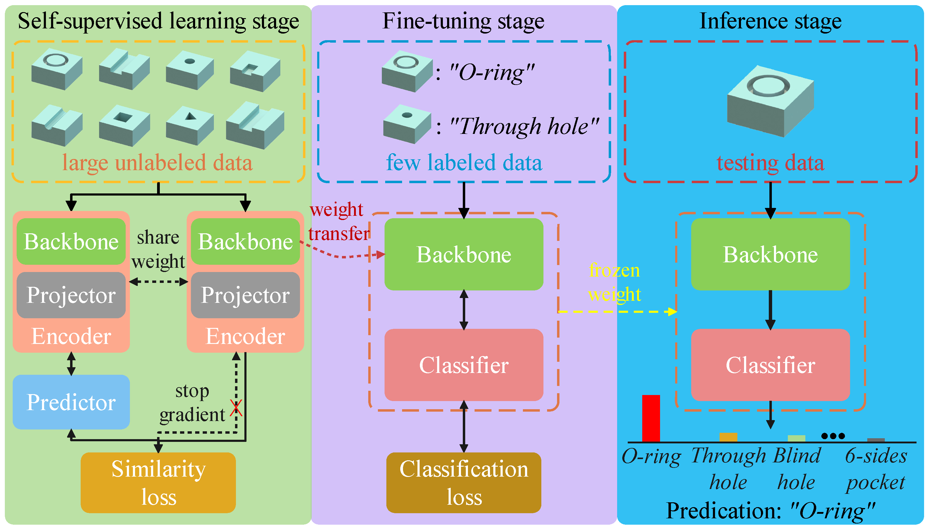
3.1. Semi-Supervised Machining Feature Recognition Framework

Semi-supervised learning, which is able to perform certain learning tasks from both labeled and unlabeled data, has made significant progress in many machine learning fields in recent years [43,44]. Motivated by the latest progress in self-supervised and semi-supervised representation learning in computer vision tasks [21,44,45,46,47], a simple and effective semi-supervised machining feature recognition framework is proposed to learn discriminative visual representation from a large amount of unlabeled data and smaller sets of labeled data. The proposed framework is concise and effective. There are only three stages: self-supervised learning, fine-tuning, and inference. In the first stage, the encoder network learns the general visual representation from large unlabeled data through self-supervised learning. In the second stage, the backbone of the encoder network is transferred to the downstream machining feature classification task, then the backbone and the classifier are fine-tuned with a few labeled data. In the final stage, the entire network’s parameters are frozen and applied to recognize machining feature. The pipeline of the proposed semi-supervised learning framework is depicted in Figure 1.

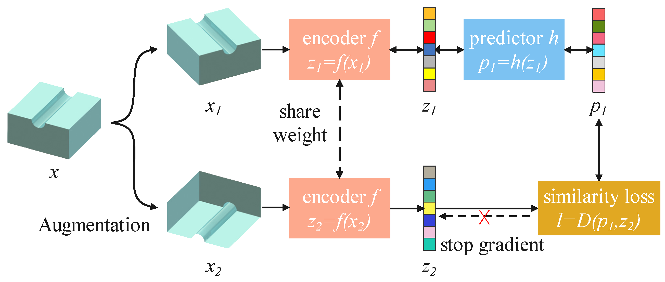
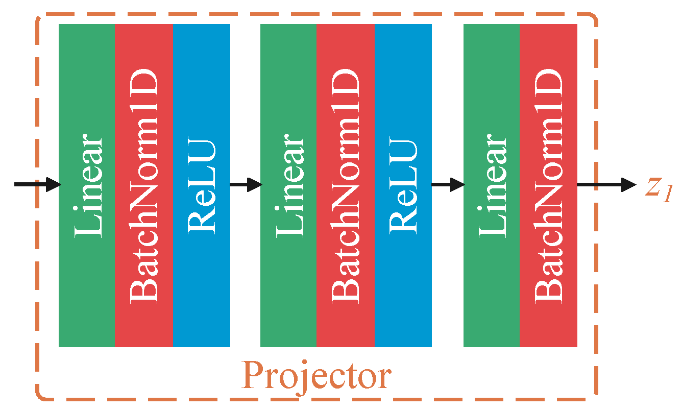
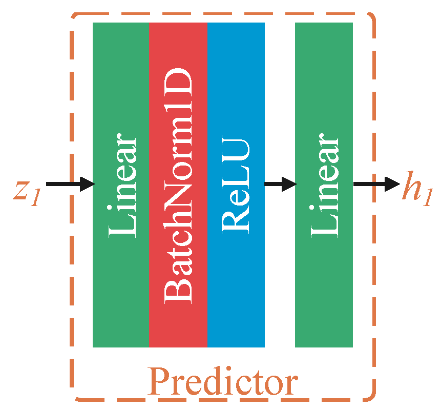
3.1.1. Self-Supervised Learning Stage

In this paper, a self-supervised learning method, similar to SimSiam [21], is proposed for machining feature recognition. SimSiam is a self-supervised learning framework that can learn meaningful visual representation without requiring a complex architecture design, momentum encoder, negative sample pairs, or large batch size. However, SimSiam is designed for 2D visual tasks (e.g., image classification, 2D object detection, 2D semantic segmentation), which cannot meet the requirement for 3D machining feature recognition. Therefore, the proposed method extends SimSiam to learn effective visual representation from a large number of unlabeled 3D machining feature data for transferring to downstream tasks. The architecture of the self-supervised learning method is shown in Figure 2.
At first, two randomly transformed (augmented) models x 1 and x 2 from a 3D model x are accepted as the architecture input. Then, the two models are fed into a shared weight encoder f composed of a CNN backbone network (e.g., ResNet-50) and a three-layer MLP projector (Figure 3). The encoder, which is in charge of projecting input into a representation space, generates two corresponding embeddings z 1 and z 2 according to x 1 and x 2 . In this process, the projector is a key component whose main function is to transform visual representation into the space where similarity loss is applied [44]. The above operations are defined as follows:
x 1 = T ( x ) , x 2 = T ( x ) , z 1 = f ( x 1 ) , z 2 = f ( x 2 ) ,
where T denotes random augmentation, and f is a shared weight encoder.
After that, one of the embeddings is sent to a predictor h (Figure 4), which returns a transformed embedding p 1 . The predictor only works on one embedding at a time, and its function is to match the output of one encoder to the other [46]. In other words, the predictor learns to predict and compensate for the difference between the outputs of two encoders. The predictor is a simple two-layer MLP, which has a similar architecture to the projector. The last batch normalization (BN) layer is removed in contrast to the projector because the BN layer causes the training results to be unstable [21]. The predictor transformation is as follows:
p 1 = h ( z 1 ) .
After the predictor, the cosine similarity criterion is used to measure the distance between the two embeddings p 1 and z 2 , which is defined as follows:
criterion ( x 1 , x 2 ) = x 1 · x 2 max ( x 1 2 · x 2 2 , ϵ ) ,
where · 2 is l 2 n o r m of a vector, and ϵ is a small value to avoid division by zero, usually 1 × 10 8 .
Correspondingly, we get z 1 and p 2 by switching the input order of x 1 and x 2 according to [46]. The above operations can be written as follows:
z 1 = f ( x 1 ) , p 2 = h ( f ( x 2 ) ) .
Now, the similarity loss is defined as follows:
l = 1 2 ( criterion ( p 1 , z 2 ) + criterion ( z 1 , p 2 ) ) ,
which is symmetric. For the symmetrized similarity loss, an intuitive explanation is to pull the two embeddings closer in a representation space by maximizing their cosine similarity (i.e., to minimize L).
Finally, error back propagation and the optimizer are utilized to compute the gradient and update the learnable parameters of the encoder and predictor. At each training step, stochastic gradient descent with momentum (SGDM) is performed to minimize the similarity loss l, which is summarized as:
v t + 1 = m v t + g t + 1 , θ t + 1 = θ t μ v t + 1 ,
where θ , g, v, μ , and m denote the parameters of network, gradient, velocity, learning rate, and momentum, respectively.
In this process, the significant stop-gradient operation (Figure 2) is used to cut off the gradient from the output of the similarity loss l to the encoder f. This operation means that the encoder f receives the gradient from the predictor h rather than directly from similarity loss l. The stop-gradient is a key to preventing the Siamese network from finding a degenerated solution as a result of collapsing [21]. Collapsing is a key concept in contrast learning, which refers to the phenomenon of the network learning to output the same embedding for all inputs, resulting in a trivial solution to the contrastive loss (i.e., the similarity loss is always optimal 1.0 ). As a result, this learning process is unable to generate gradient in order to update the network parameters and learn any valid visual representation.
In summary, the method is a simple self-supervised learning framework, requiring only a few extra modules (projector and predictor) and operation (cosine similarity and stop-gradient). Intuitively, Siamese networks maximize the agreement between two randomly augmented views from a 3D model, enabling the encoder network to ignore irrelevant information and learn distinguishable visual representation. In practice, we can easily use this approach to pre-train a visual encoder on large amounts of unlabeled data and then transfer to the downstream task (e.g., machining feature recognition).

3.1.2. Fine-Tuning

After the self-supervised learning stage, the encoder has a certain level of feature extraction capability and is able to extract discriminative representation from a 3D model. To use the knowledge gained from a self-supervised task, transfer learning is adopted to enhance the performance of the downstream task. Specifically, a small amount of labeled data is utilized to fine-tune the transferred backbone and train the classifier. This procedure is very simple and the same as multi-classification training.
During the fine-tuning stage, we keep only the parameters of the backbone network (as shown in Figure 1) and discard the parameters of other layers. First, the backbone network receives a 3D model and outputs a corresponding embedding vector. Then, the vector is sent to the softmax classifier that consists of a fully connected (FC) layer and a softmax function. The softmax is defined as follows:
Softmax ( x ) = e x p ( x i ) i = 1 N e x p ( x i ) ,
where x is a 1D vector, and N is the length of the vector (equal to the number of classes defined in the dataset).
The final output of the classifier is a probability distribution over predicted classes. In the end, cross-entropy (CE) loss is applied between the predicted probability distribution and the one-hot label. The CE loss is defined as follows:
CE ( y , y ) = i = 1 N y i log ( y i ) ,
where N is the number of class, y i denotes the prediction probability of a sample belonging to class i, and y i is the one-hot vector label, when l a b e l = i , y i = 1 , otherwise y i = 0 . An SGDM optimizer is employed to minimize the loss function and update the parameters of the network. It is important to note that we adopt different learning rates for the backbone and the classifier in order to prevent the transferred knowledge from being destroyed while achieving rapid convergence. The initial learning rate is set to 1 × 10 3 for the backbone and 30.0 for the classifier. To summarize, the classifier is the final component that is used to learn the mapping between the embedding vector and the real value.

3.1.3. Inference Stage

In the inference stage, the parameters of the entire network are frozen and prepared for deployment. Three-dimensional models from CAD are fed into the network to obtain the probability distribution corresponding to predicted classes so as to identify the category of machining feature.

3.2. Lightweight CNN Models for Machining Feature Recognition

As noted in the introduction, current machining feature recognition networks have large parameters and many floating-point operations per second (FLOPs). These large networks take up a lot of memory and become challenging to achieve fast inference speed on personal computers. In addition, a better computer with faster GPU(s) and more graphic memory is needed to train a large network, so more money must be spent on hardware. Motivated by recent excellent mobile networks [48,49,50], this paper applies some lightweight techniques to neural networks for addressing the above problem, with the goal of maintaining high recognition accuracy while reducing inference latency and memory usage. The following part introduces FeatureNetLite and MsvNetLite, which are the lightweight versions of FeatureNet and MsvNet.

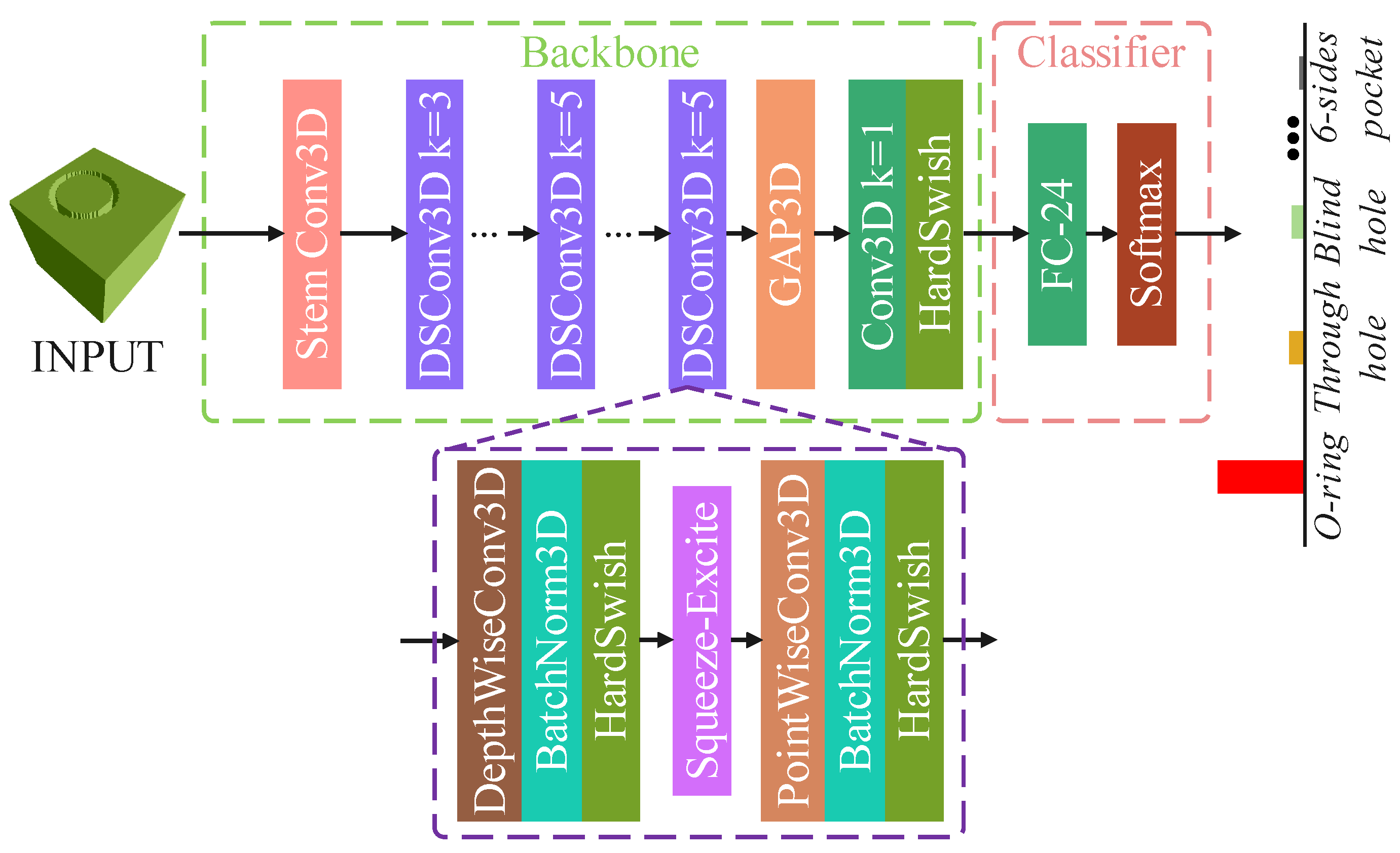
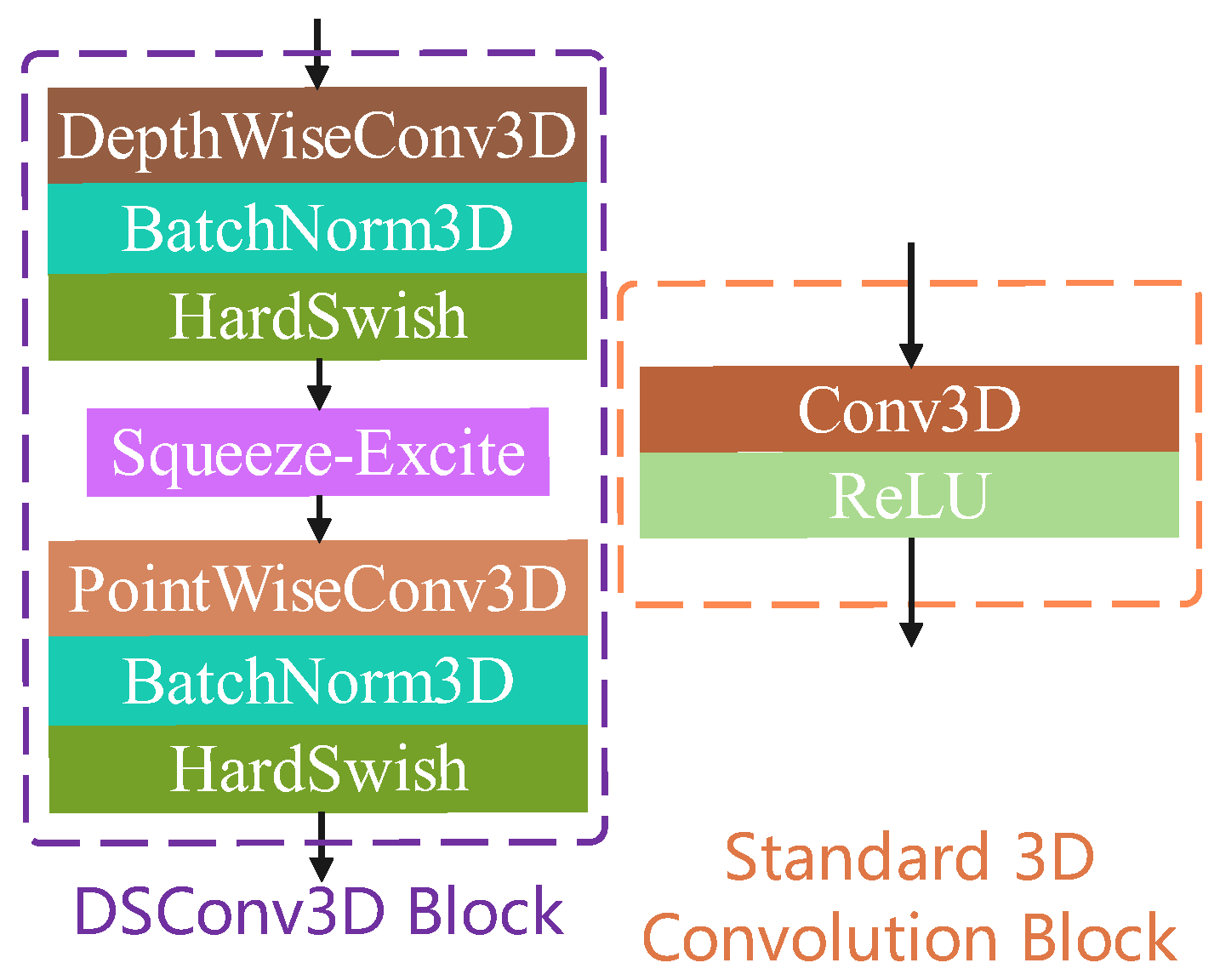
3.2.1. FeatureNetLite
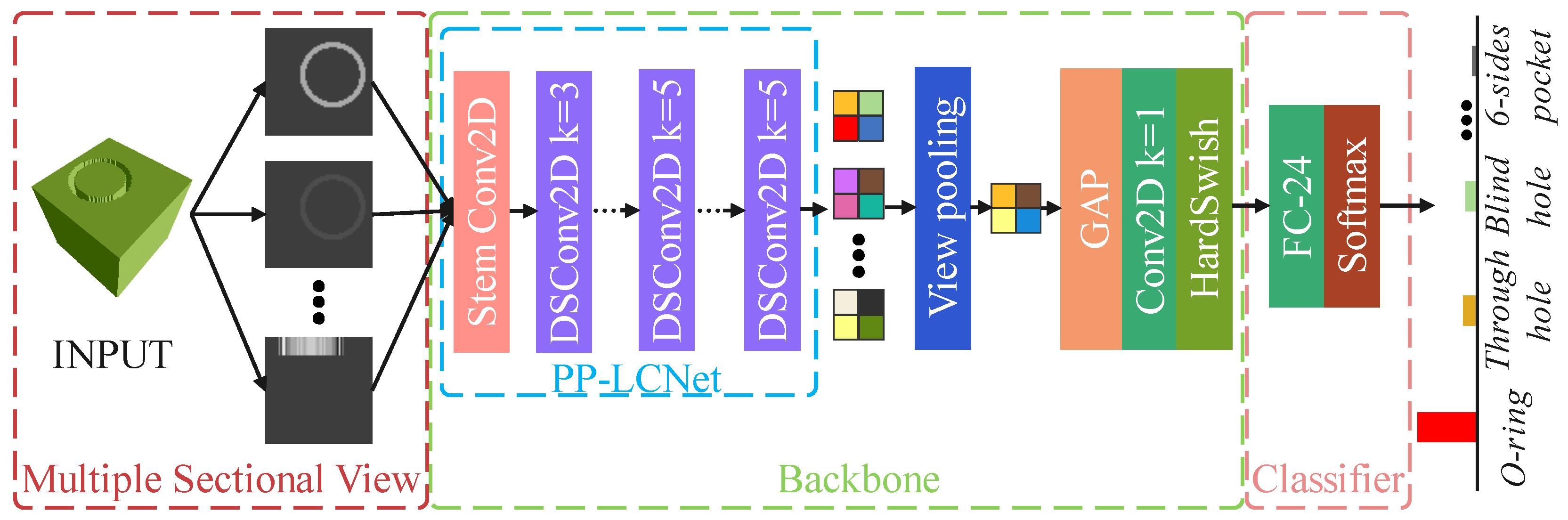
To our best knowledge, Ref. [14] first attempted to apply 3D CNN to machining feature recognition and proposed voxel-based FeatureNet. Voxel is a concept in 3D computer graphics that refers to a 3D grid that represents the occupancy of space within an object. However, FeatureNet has a lot of parameters (33.94 M) and FLOPs (12.51 G), so we apply lightweight techniques to it and propose FeatureNetLite. The topological architecture of the proposed FeatureNetLite is similar to PP-LCNet [50]. However, PP-LCNet is designed for 2D image classification and incompatible with our 3D voxel machining feature classification task. Therefore, this paper modified the convolution block of the network to allow for accepting 3D voxel input with fewer parameters (1.91 M) and lower FLOPs (0.14 G). As depicted in Figure 5, the FeatureNetLite consists of two parts:
The first part is a CNN backbone for feature extraction, which contains a stem Conv3D block, multiple depth-wise separable convolution 3D (DSConv3D) blocks, a global average pooling 3D (GAP3D) layer, and a Conv3D layer after GAP3D. As the core of the entire network, DSConv3D is a 3D variant of depth-wise separable convolution [51], which is widely used in mobile networks. In FeatureNetLite, the DSConv3D block is used instead of a standard 3D convolution block, allowing the network to significantly increase computation efficiency while preserving the same learning capability. Additionally, the DSConv3D block makes the convolutional layers more sparse, which can effectively avoid overfitting. Figure 6 shows the difference between the DSConv3D block and a standard 3D convolution block.
The DSConv3D block is composed of depth-wise convolution 3D [52], batch normalization 3D [53], point-wise convolution 3D [52], and HardSwish nonlinear activation function [49].
At the head of block, there is a depth-wise convolution 3D, which only uses one convolutional kernel for each input channel. After the depth-wise convolution 3D, BatchNorm3D is applied to reduce internal covariate shift and speed up the training process. Aiming at better quality of the activation function, ReLU is replaced by HardSwish, which can significantly increase performance while avoiding a large number of exponential operations. The HardSwish activation function is defined as follows:
HardSwish ( x ) = 0 , x 3 x , x 3 x ( x + 3 ) 6 , o t h e r w i s e
In addition, a Squeeze-and-Excite (SE) module [54] is added to DSConv3D blocks to improve recognition performance. The SE is a channel attention module that enables the network to pay more attention to the channel with important information and less to irrelevant information. However, extensive use of an SE module results in a significant increase in inference time. To keep the balance between accuracy and inference speed, the SE module is only added to the blocks near the tail of network. Subsequently, point-wise convolution 3D, whose kernel size is set to 1, is applied to compute the weighted combination of the output of the depth-wise convolution 3D.
Due to the above designs, the parameters and computational complexity of DSConv3D are significantly reduced compared to a regular convolution layer. The last Conv3D layer with kernel size set to 1 lifts up the output of network from 512 × 1 3 to 1280 × 1 3 , which slightly increases inference time but greatly improves nonlinear fitting ability.
The second part involved in the network is a softmax classifier, which is commonly adopted in multi-classification task. The classifier only contains a fully connected (FC) layer and a softmax nonlinear activation function. The output dimension of the classifier is the number of machining feature classes in FeatureNet dataset.
The detailed configuration of FeatureNetLite is shown in Table 1. The parameter s t r i d e controls the stride size for the convolution operator. The s t r i d e controls the stride size for the convolution operator. When s t r i d e set to 1, it is a plain convolution and does not change the resolution of the output feature map. When s t r i d e set to 2, the layer performs a down-sampling operation. The dimension order of the convolution output is c h a n n e l × h e i g h t × w i d t h × d e p t h ( C × H × W × D ).

3.2.2. MsvNetLite

Another well-known machining feature recognizer is MsvNet [20], which is a multi-view based approach. Multi-view is a method to represent a 3D object through multiple 2D images from different viewpoints. Similar to FeatureNet, MsvNet also has a large number of parameters (128.86 M) and FLOPs (7.46 G). Therefore, we present a lightweight CNN called MsvNetLite, whose architecture is similar to MsvNet. MsvNetLite can be considered a lightweight and modernized version of MsvNet (only 1.70 M parameters and 0.16 G FLOPs). Compared to MsvNet, the most significant change in MsvNetLite is the replacement of the 2D CNN backbone network from VGGNet-11 [55] to PP-LCNet [50]. Furthermore, a smaller MLP takes the place of the original large MLP as the final classifier. After the aforementioned adjustments, the recognition performance also shows strong competitiveness while using fewer parameters and FLOPs. As shown in Figure 7, this network takes multiple sectional views (MSV) representation as input. In MSV, many 2D images are taken from a variety of viewpoints to represent a 3D voxel model. The detailed configuration of MsvNetLite is shown in Table 2. The Stem Conv2D block contains Conv2D, BatchNorm2D, and HardSwish layers. DSConv2D denotes a depth-wise separable convolution block [50]. The view pooling layer uses an element-wise max operator to combine all embeddings into one embedding [56]. The dimension order of convolution output is v i e w × c h a n n e l × h e i g h t × w i d t h ( V × C × H × W ).

4. Experimental Results

In order to assess the performance of the proposed semi-supervised learning framework on a small labeled dataset, this section presents extensive experimental results for machining feature recognition. Furthermore, the lightweight CNN networks FeatureNetLite and MsvNetLite are compared to other DL-based machining feature recognizers to demonstrate the advantages of the proposed approaches.

4.1. Experimental Settings

In this experiment, the FeatureNet dataset (see Figure 8), which contains 144,000 (24 classes × 1000 models × 6 orientations) different CAD models stored in stereolithography (STL) files, is used as a benchmark. Because the approaches involved in the comparisons only accept 3D voxels as input, the STL files must be converted to binvox data format [14]. In addition, the MSV representation is captured from the voxel grid and also requires voxel as input [20]. In this study, 3D CAD models are voxelized in a 64 × 64 × 64 grid resolution. For fair comparison, the entire dataset is divided into a training set (80% of the total dataset), a validation set (10%), and a test set (10%) in accordance with [20]. All the training tasks were conducted on a cloud server with Intel Xeon Gold 6230R CPU, 32 GB memory, and NVIDIA Tesla V100S (32 GB) GPU. For reasonable comparison on personal computer, all the latency testing tasks were carried out on a consumer laptop with Intel Core i7-7700 CPU, 16 GB memory, and NVIDIA GeForce GTX 1070 (8 GB) GPU. All experiments were implemented on PyTorch 1.9.0 [57]. The inference latency values are the average over 1000 runs.
Accuracy, which is a widely used metric in machine learning, is used to evaluate the performance of the approaches. It measures the proportion of correctly classified instances among all instances in the dataset. Its simplicity and ease of interpretation make it a popular choice, particularly for balanced classification problems. Accuracy is defined as follows:
Accuracy = Number of correctly classified instances Total number of instances

4.2. Effectiveness of the Proposed Semi-Supervised Learning

We performed ablation experiments of the proposed semi-supervised learning framework over FeatureNetLite and MsvNetLite to demonstrate its improvements. The training settings and strategies of MsvNet and MsvNetLite were the same as those proposed by [20]. FeatureNet and FeatureNetLite also followed the configuration recommended by [14]. Detailed training settings are as follows:
  • MsvNetLite, FeatureNetLite, FeatureNet, Baseline1, Baseline2, and VoxNet underwent 100 epoch training. The MsvNet was trained with 120 epochs. This is because Shi et al. adopted a two-stage training strategy, initially training the network 20 epochs on the single view of a voxel model.
  • MsvNetLite and FeatureNetLite using semi-supervised learning were trained by an SGDM optimizer with 1 × 10 6 weight decay. MsvNet, FeatureNet, Baseline1, Baseline2, and VoxNet were trained by an Adam optimizer [58] without weight decay.
  • The mini-batch size was set to 64. The batch size is limited to the number of training data if the number of training data is less than the batch size.
  • The initial learning values of MsvNetLite and FeatureNetLite using semi-supervised learning were set to 1 × 10 3 for the backbone and 30.0 for the classifier, and a cosine learning rate decay scheduler was used. MsvNet, FeatureNet, Baseline1, Baseline2, and VoxNet were trained with an initial learning rate set to 1 × 10 3 and no decay scheduler.
  • According to [20], the following data augmentation strategies were also adopted in our experiments: Random Rotation, Random Scale, and Random PadCrop.
  • For fair comparison with [20], the number of sectional views was set to 12 for multi-view approaches.
  • FeatureNetLite using semi-supervised learning was trained 50 epochs in the self-supervised stage, and MsvNetLite using semi-supervised learning was trained 100 epochs in the self-supervised stage.
To examine the generalization performance of the proposed framework on small labeled samples, we evaluated several approaches on the different numbers of labeled data per class for training. For example, when the number of labeled data per class is set to 1, only 24 labeled samples (24 classes × 1 sample per class) are used to train the network. Detailed hyper-parameter settings about semi-supervised learning are discussed in Section 4.5. The comparative results are shown in Table 3: P T denotes initializing the 2D CNN backbone with ImageNet pre-trained weights provided by torchvision and [50], D A denotes adopting Random Rotation, Random Scale, and Random PadCrop data augmentation during supervised training, and Semi-Sup. denotes applying semi-supervised learning framework on the approach.
In the result table, the bold font presents the best accuracy for the test set for each column. It is observed from this table that MsvNetLite has significantly improved accuracy on small amounts of labeled data (≤16) with the application of semi-supervised learning. In particular, with just one training sample per class, MsvNetLite performed about 24% better with semi-supervised learning than without semi-supervised learning. Even when compared to the huge network MsvNet, this represents a 19% improvement. However, we can observe that MsvNetLite with semi-supervised learning does not improve performance with a large amount of training data (≥64), but rather slightly degrades it. This may be because the visual representation learned in the self-supervised learning stage is not so robust. As we can see from Table 3, FeatureNetLite with semi-supervised learning is significantly improved with the different numbers of training data and also outperforms other voxel-based approaches. Similar to the experimental results from [20], the classification performance of the voxel-based approach is not comparable with the MSV-based approach. Additionally, the results show that data augmentation and ImageNet pre-trained weight also can improve accuracy on small labeled sample learning. This is because data augmentation introduces variations to the dataset to help the model generalize better. In addition, pre-trained weights transfer the knowledge gained from other datasets (e.g., ImageNet) to the task of recognizing machining features.

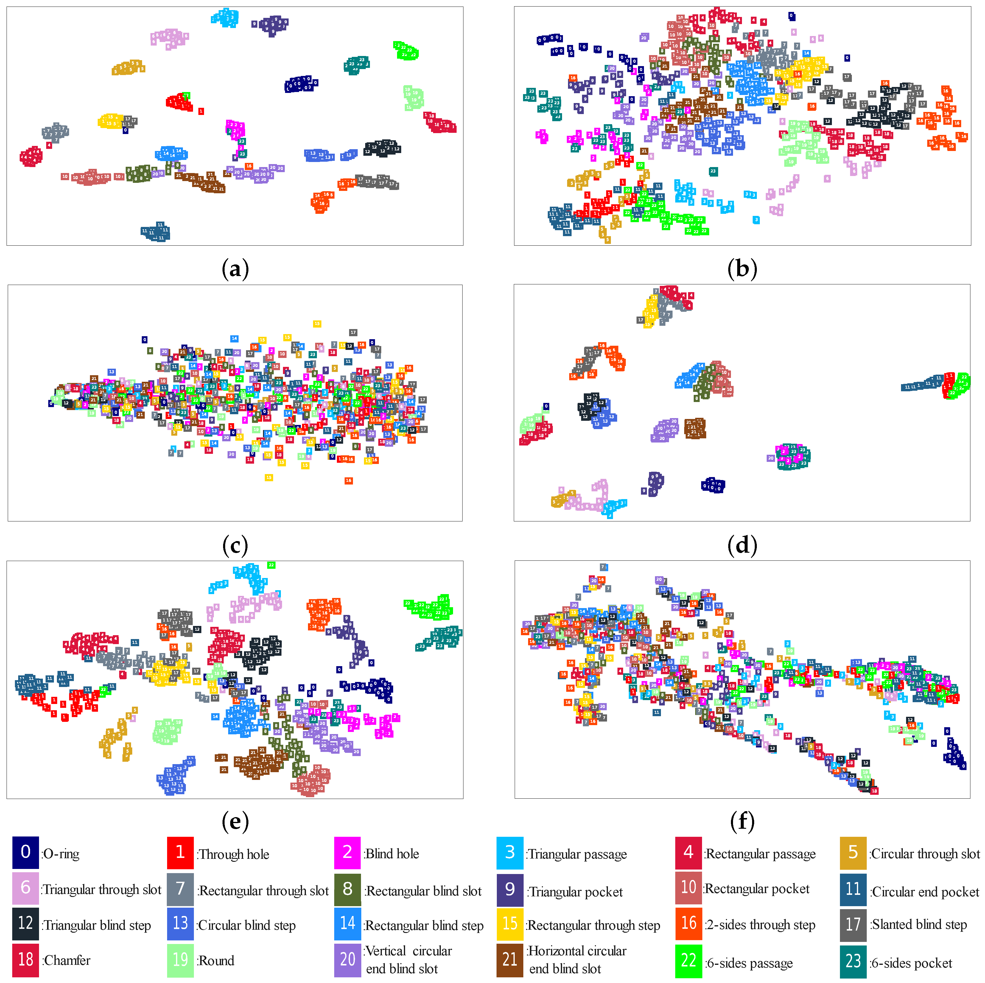
4.3. Visualization of the Visual Representation

To explore the effectiveness of the proposed semi-supervised learning framework, we visualized the visual representation produced by the last layer (after the flatten layer) of the backbone using t-SNE [60]. With 40 test samples per class as input, we first extracted the deep visual representation. Next, we utilized t-SNE to reduce the dimension of visual representation from 1280D to 2D. Finally, the 2D representation was plotted on a 2D plane. All experiments were based on MsvNetLite. In semi-supervised learning, 144,000 unlabeled samples were used for self-supervised learning and only 192 labeled samples for fine-tuning. In supervised learning, only 192 labeled samples were used for training. The parameters of t-SNE were set as follows: p e r p l e x i t y = 100 , i t e r a t i o n s = 500 , and i n i t i a l i z a t i o n = p c a .
The t-SNE visualization results are shown in Figure 9. Different colors and numbers stand for different class labels corresponding to Figure 8. For intuitive evaluation, we visualized the reduced embeddings of six situations: (a) the backbone output of MsvNetLite after fine-tuned using the SGDM optimizer in semi-supervised learning, (b) the backbone output of MsvNetLite initialized with ImageNet pre-trained weights, (c) the backbone output of MsvNetLite with random initialization, (d) the backbone output of MsvNetLite after self-supervised stage in semi-supervised learning, (e) the backbone output of MsvNetLite after supervised learning, and (f) the backbone output of MsvNetLite after fine-tuned using the Adam optimizer in semi-supervised learning.
In Figure 9a, after semi-supervised learning, the embeddings seem to cluster, and 24 well-separated clusters can be seen. In Figure 9b, the backbone is only trained on the ImageNet and never sees the FeatureNet dataset. Although the embeddings look indistinguishable and are not clearly separated, some of them appear to cluster together. This presents an intuitive explanation for knowledge transferring. Figure 9c shows the representation from the backbone without training, in which the embeddings look chaotic and random. In Figure 9d, multiple distinct clusters can be seen after self-supervised learning, which indicates that self-supervised learning produces meaningful visual representation even without the use of labeled data. However, we can still observe that some class overlapping exists. These results demonstrate that the self-supervised learning helps network in class separation and learn discriminative visual representation even without labeled data. Figure 9e depicts the representation from the backbone trained with supervised learning. We can observe that the embeddings produced by the supervised backbone are more indistinguishable and not separated well in comparison to Figure 9a. Therefore, the proposed semi-supervised learning produces high-quality representation and better class separation, validating its effectiveness in improving recognition performance. Figure 9f presents a fail case where the Adam optimizer is used for fine-tuning. We can see that the majority of the embeddings become random and indistinguishable, which may indicate that the knowledge from self-supervised learning is lost. In Section 4.5.5, there is a detailed discussion about why the Adam optimizer is unable to fine-tune.

4.4. Efficiency of the Proposed FeatureNetLite and MsvNetLite

The second experiment was carried out to evaluate the efficiency of the proposed lightweight neural networks. We compared optimal accuracy, parameters, FLOPs, and inference latency with other learning-based machining feature recognition approaches. Optimal accuracy is the highest achievable accuracy attained by a particular approach. In the context of our study, the optimal accuracy was determined by examining the results presented in Table 3. For instance, upon analysis of Table 3, it was observed that MsvNetLite achieved the highest accuracy value of 98.84, therefore, the optimal accuracy of MsvNetLite is considered to be 98.84. Additionally, we have included confusion matrices and receiver operating characteristic (ROC) curves for each approach to more thoroughly analyze the distinctions in classification performance. The confusion matrices and ROC curves are shown in Appendix A.
In Table 4, FeatureNetLite achieves nearly 18 × reduction in parameters and 89 × reduction in FLOPs compared to FeatureNet and even outperforms other voxel-based approaches in classification performance. Similarly, when compared to MsvNet, MsvNetLite has only 1 / 76 parameters and 1 / 47 FLOPs, but their classification performances are approximately equivalent (about −0.3%). Furthermore, this table also shows the results of the inference latency tested on I7-7700@3.6GHz CPU and GTX1070 GPU. Both on the CPU and GPU, FeatureNetLite is more than twice as fast as FeatureNet in inference speed. When compared to MsvNet, the inference speed of MsvNetLite is just 2 ms faster on the GPU but over six times faster on the CPU. Although the proposed networks are neither the fastest nor the most accurate, they achieve the best balance between accuracy and inference speed. It has been noted that the acceleration effects of the two lightweight networks on CPU and GPU are not consistent, which is caused by the disparate hardware architecture. As GPU is likely used to render 3D objects in CAD software, inference speed on CPU is more significant. In general, fewer network parameters and faster inference speed mean lower memory usage and quicker response of machining feature recognition application, respectively.

4.5. Discussion about the Hyper-Parameters of the Proposed Semi-Supervised Learning

In this subsection, we further study the hyper-parameter settings of the proposed semi-supervised learning in order to determine the optimal semi-supervised training settings. All experiments are based on MsvNetLite.

4.5.1. Different Numbers of Unlabeled Data in Self-Supervised Stage

The impact of different amounts of unlabeled data in self-supervised learning was examined. In this experiment, the setups of self-supervised training, the predictor, and the projector were based on [21]. The batch size was set to 32, the base learning rate at 6.25 × 10 3 with a cosine decay scheduler (but we fixed the learning rate of the predictor), the weight decay at 1 × 10 4 , all data augmentations (Random Rotation, Random Scale, and Random PadCrop) enabled, and the training epoch at 100 with an SGDM optimizer ( m o m e n t u m = 0.9 ) for self-supervised training. In the fine-tuning stage, the initial learning rate of the classifier was set to 30 with a cosine decay scheduler [61], the weight decay at 1 × 10 6 , only Random Rotation augmentation enabled, the train batch size at 64 (the batch size is limited to the number of training data if the number of training data is smaller than the batch size), and the fine-tuning epoch at 100 using the SGDM optimizer ( m o m e n t u m = 0.9 ).
The results are shown in Table 5. This table clearly shows that using more unlabeled data for self-supervised training increases the accuracy of the fine-tuning stage. More data for training means being able to learn better visual representation, but it also requires collecting more data and more training time. Of course, it costs nothing to collect large amounts of unlabeled data.

4.5.2. Different Batch Size for Self-Supervised Learning

We discussed the effect of different batch size in the self-supervised stage. In this experiment, according to the linear scaling rule [62], the learning rate changed according to the batch size. The rule of learning rate change was as follows:
lr = base _ lr × BatchSize 256
where the base_lr denotes base learning rate, which was set to 5 × 10 2 . The remaining experimental settings were the same as the previous experiment.
The results with a batch size for self-supervised learning from 16 to 256 are reported in Table 6. This result shows that the optimal fine-tuning accuracy is obtained when the batch size was set to 32 for self-supervised learning. We also observe that there is a serious performance drop when the batch size increases from 64 to 256. When the batch size decreases to 16, there is a small performance change within the level of random variations. It is worth noting that these results are obtained from our training on the FeatureNet machining feature dataset and do not represent a consistent performance on other datasets.

4.5.3. Different Training Epochs in Self-Supervised Stage

The effect of different training epochs for self-supervised learning was explored. In this experiment, the training epochs for self-supervised learning were set to 50, 100, and 200. The other experimental setups were the same as in the first experiment.
The results are reported in Table 7. The results show that the accuracy increases with the increase of training epochs when fine-tuning with a very small number of labeled samples (≤2). However, 100 epochs self-supervised training show the best accuracy when the number of labeled samples is larger than 2. Usually, longer self-supervised training allows the encoder to learn more distinguishable visual representations. However, this phenomenon suggests that self-supervised learning may be sensitive to the setting of some hyper-parameters.

4.5.4. Different Data Augmentation Strategies in Self-Supervised Stage

Three widely utilized augmentations were used to systematically study their effects on self-supervised learning. The data augmentations evaluated in this experiment involved spatial and geometric transformations of a 3D object, including Random Rotation, Random Scale, and Random PadCrop. The rest of thr experimental settings were the same as in SubSection 4.5.1.
Table 8 reports the accuracy under different compositions of data augmentations. As can be seen, enabling all data augmentation strategies results in the best accuracy. With only one data augmentation, the worst performance is attained. Obviously, using more data augmentation improves recognition performance. We conjecture that more data augmentation strategies further remove some redundant information to ensure that the learned representation has better generalization ability. In other words, with more spatial and geometric transformations, the encoder network is forced to concentrate more on the important information within the input data.

4.5.5. Different Optimizers for Fine-Tuning

As noted in Section 4.2, the SGDM optimizer is used instead of Adam in the fine-tuning stage. The following empirical study shows the influence of different optimizers for fine-tuning. The epochs of self-supervised learning were 100, and the remaining setups were the same as in Section 4.5.1. In the fine-tuning stage, the batch size was set to 64. The learning rates of the backbone and the classifier were set to 30 and 1 × 10 3 , respectively, with a cosine decay scheduler. Random Rotation, Random Scale, and Random PadCrop augmentation strategies were used. The optimizers involved in the experiment included Adam, stochastic gradient descent with momentum (SGDM), stochastic gradient descent (SGD), and RMSProp without the weight decay. All the training was conducted for 100 epochs.
The results are shown in Table 9. SGDM achieves the best testing accuracy, and the performance of SGD slightly drops. However, Adam and RMSProp show a significant reduction in performance and seem to lose the knowledge transferred from self-supervised learning during fine-tuning. Adam and RMSProp are both adaptive learning rate approaches that can adjust the learning rate of each learnable parameter dynamically. We conjecture that their adaptive learning rate property results in the loss of learned representation. Possible future research is to explore what causes this phenomenon.

4.6. Critical Analysis and Discussion

In conclusion, the proposed approaches presented in this paper offer a promising solution to the challenges of DL-based machining feature recognition. There are some advantages to be highlighted. The proposed semi-supervised learning framework is able to leverage both labeled and unlabeled data to improve machining feature recognition. With the help of the framework, the MsvNetLite and the FeatureNetLite obviously surpassed the large models such as MsvNet and FeatureNet. The proposed framework can be a promising approach to improving the recognition performance of user-defined machining feature while minimizing the need for manual labeling. Moreover, the utilization of model compression techniques can significantly reduce the model parameters and computing complexity, making the models CPU-friendly and more suitable for real-world industrial applications. This can lead to improved software execution efficiency and lower hardware costs.
However, there are also limitations of the proposed approaches presented in this paper, which must be taken into consideration when applying them to real-world applications. First, the evaluation of the proposed approaches was limited to the FeatureNet dataset, which may not necessarily represent the complexity and diversity of other datasets. Therefore, further investigation and validation on a wider range of datasets is necessary to generalize the effectiveness of these approaches. Second, the requirement of a considerable amount of training time for the current self-supervised stage may incur additional costs in terms of time and resources. Hence, it is important to assess the training budget for implementing the approach in real-world CAPP.

5. Conclusions and Future Work

This paper presents a novel and effective approach to the task of machining feature recognition with limited labeled samples through the use of a semi-supervised learning framework. The key contribution of this framework is the incorporation of self-supervised learning, which enables the learning of useful visual representations from large-scale unlabeled data. Then, the backbone network is fine-tuned with small labeled data, utilizing the knowledge gained from self-supervised learning. Ablation experiments were performed to demonstrate the effectiveness of the proposed method. The MsvNetLite outperformed the MsvNet by approximately 19% with only one training sample per class, whereas the FeatureNetLite outperformed the FeatureNet by about 20% in machining feature classification. The t-SNE visualization technique was used to provide an intuitive visualization of the effects of the proposed framework on class separation and visual representation learning. Additionally, a large number of hyper-parameter search experiments were conducted to select the optimal semi-supervised learning settings for machining feature recognition.
Moreover, lightweight techniques were applied to the CNNs to reduce memory usage and increase inference speed. Our study shows that the proposed compressing approaches have effectively reduced the model parameters and computing complexity of the current approaches. Specifically, the MsvNetLite demonstrated a 1/76 reduction in parameters and a 1/47 reduction in FLOPs compared to the MsvNet, whereas the FeatureNetLite showed a 1/89 reduction in parameters and a 1/18 reduction in FLOPs compared to the FeatureNet. These results highlight the efficiency of our proposed compressing approaches. On a common X86 CPU, the MsvNetLite demonstrated 6.68× improvement in speed over the MsvNet, and the FeatureNetLite was 2.49× faster than the FeatureNet in terms of inference speed. The proposed models were proven to be more efficient in comparison to several other machining feature recognition algorithms, achieving the best balance between classification performance and inference speed.
However, there are some future research directions as follows:
  • Better self-supervised representation learning methods will be explored. In the future, we will improve the effectiveness of the self-supervised training stage to learn more stable pre-trained knowledge.
  • We will continuously focus on the robustness of semi-supervised hyper-parameters. We will carry out a series of experiments with different hyper-parameters to understand how the hyper-parameters effect the training process.
  • Our further research will consider the application of multiple, intersecting, and incomplete feature recognition. We will try to use the proposed approach to boost the performance of the current intersecting feature recognition method.
Therefore, we will carry on improving our framework in future work.

Author Contributions

Conceptualization, H.W. and Y.P.; Data curation, H.W.; Formal analysis, H.W.; Funding acquisition, Y.P.; Investigation, H.W.; Methodology, H.W.; Project administration, Y.P.; Resources, R.L.; Software, H.W. and R.L.; Supervision, P.H. and Y.P.; Validation, H.W., R.L., and Y.P.; Visualization, H.W.; Writing—original draft, H.W.; Writing—review and editing, H.W., R.L., P.H., and Y.P. All authors have read and agreed to the published version of the manuscript.

Funding

This work was sponsored by the National Key Research and Development Program of China (No.2022YFB3304100).

Institutional Review Board Statement

Not applicable.

Informed Consent Statement

Not applicable.

Data Availability Statement

All the related code and data generated during this research are included in the article, and the code and the data that support the conclusion of this study are openly available at https://github.com/whjdark/ssl_for_MFR (accessed on 1 February 2023).

Acknowledgments

The computation is completed in the HPC Platform of Huazhong University of Science and Technology.

Conflicts of Interest

The authors declare no conflict of interest.

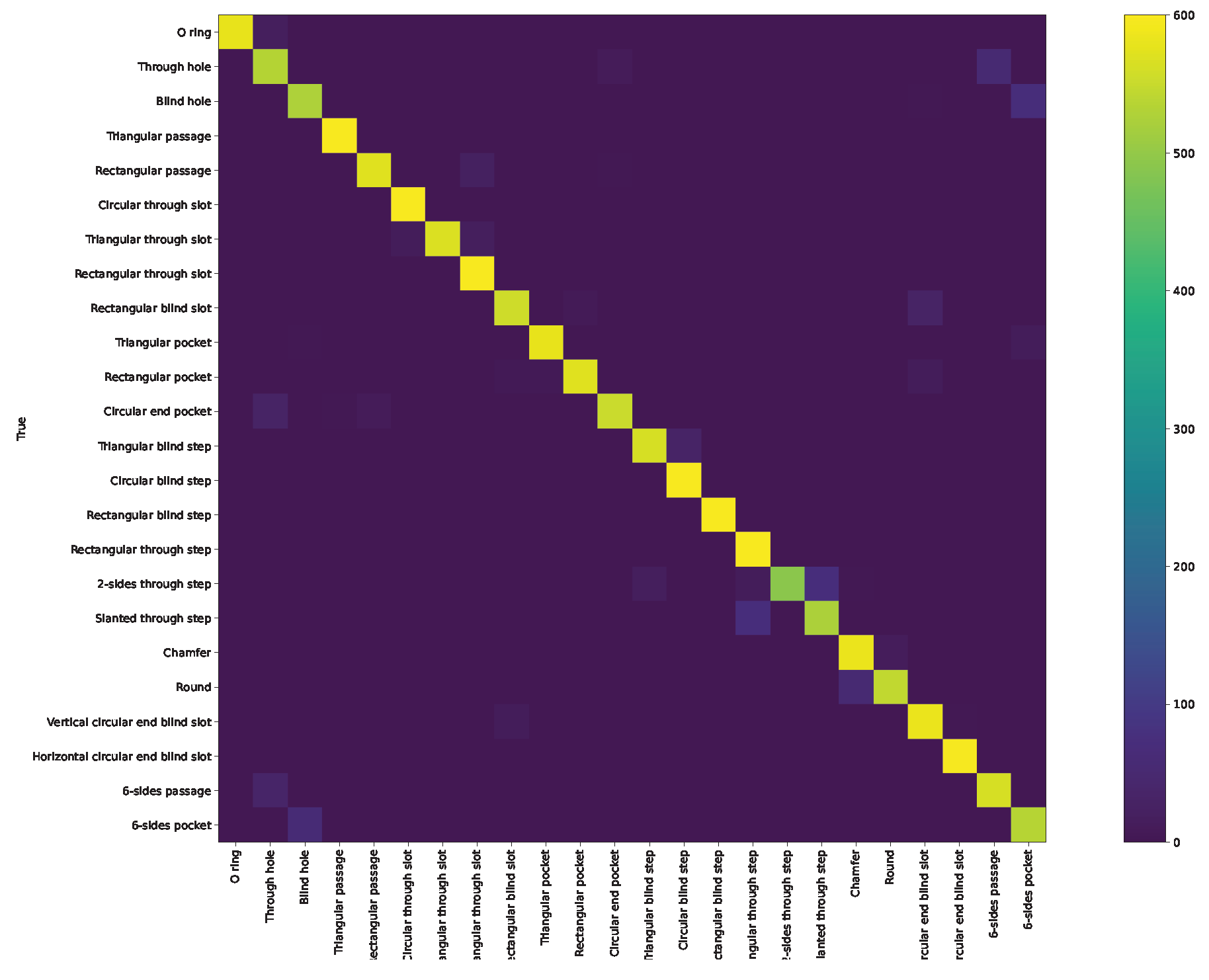
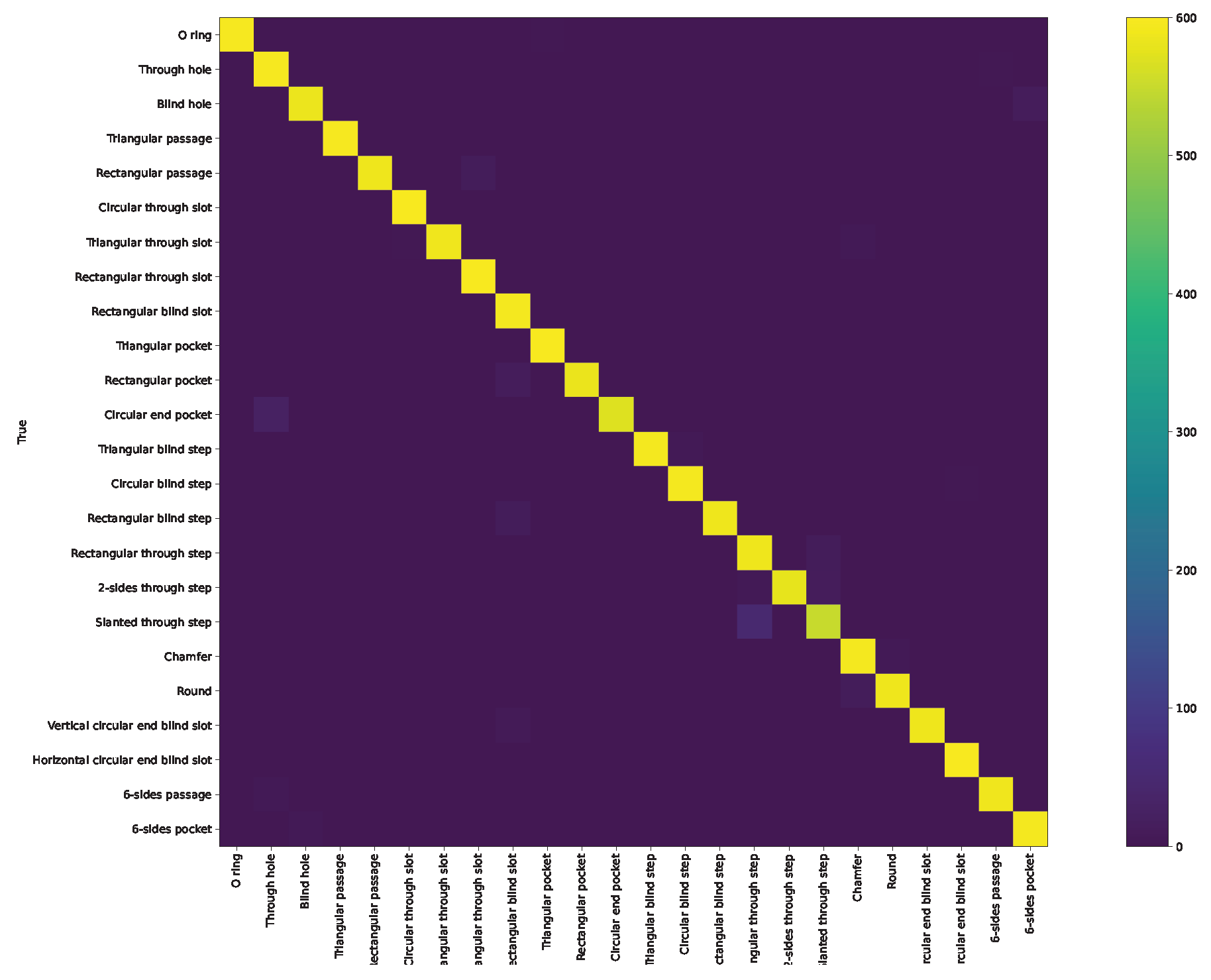
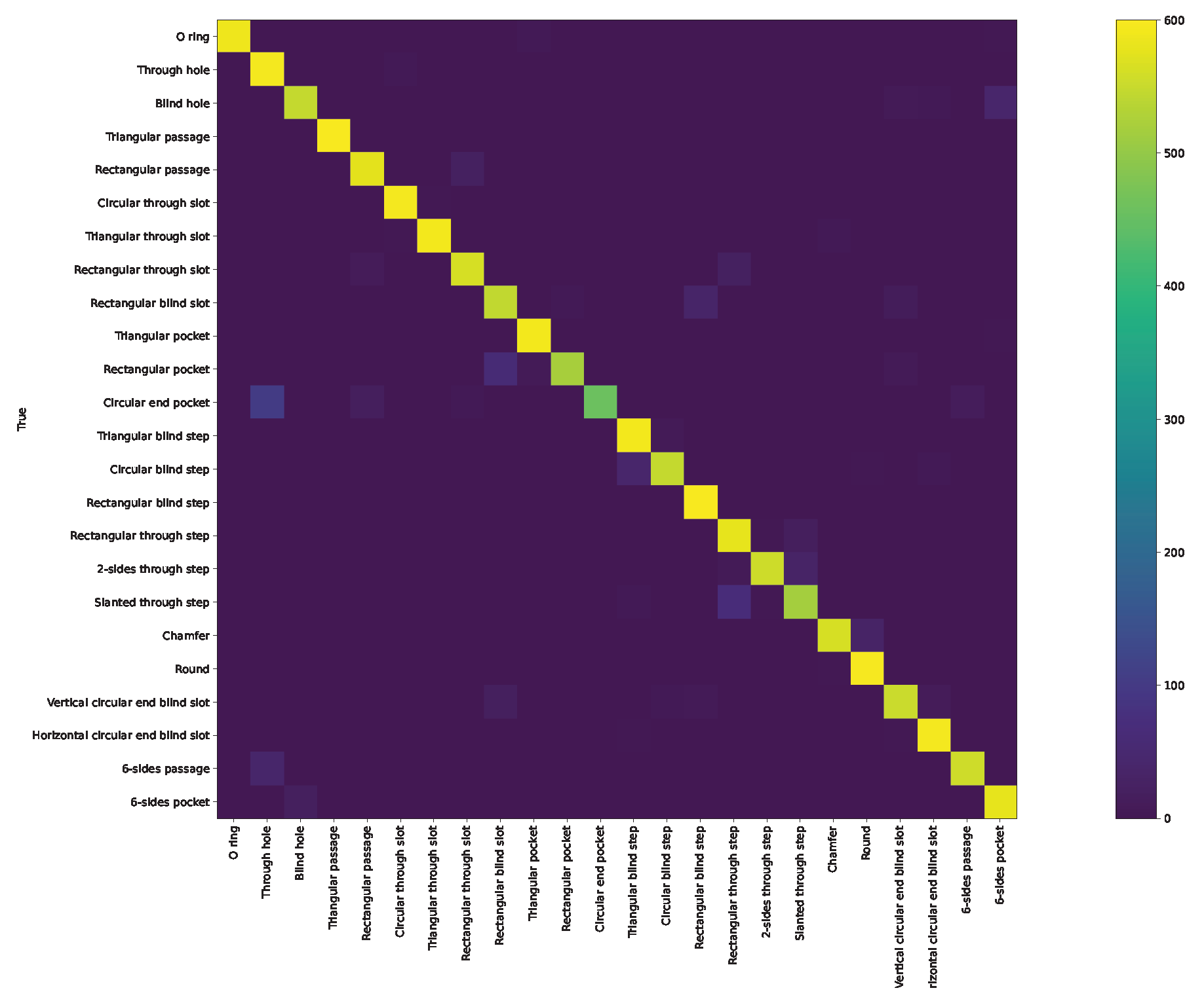
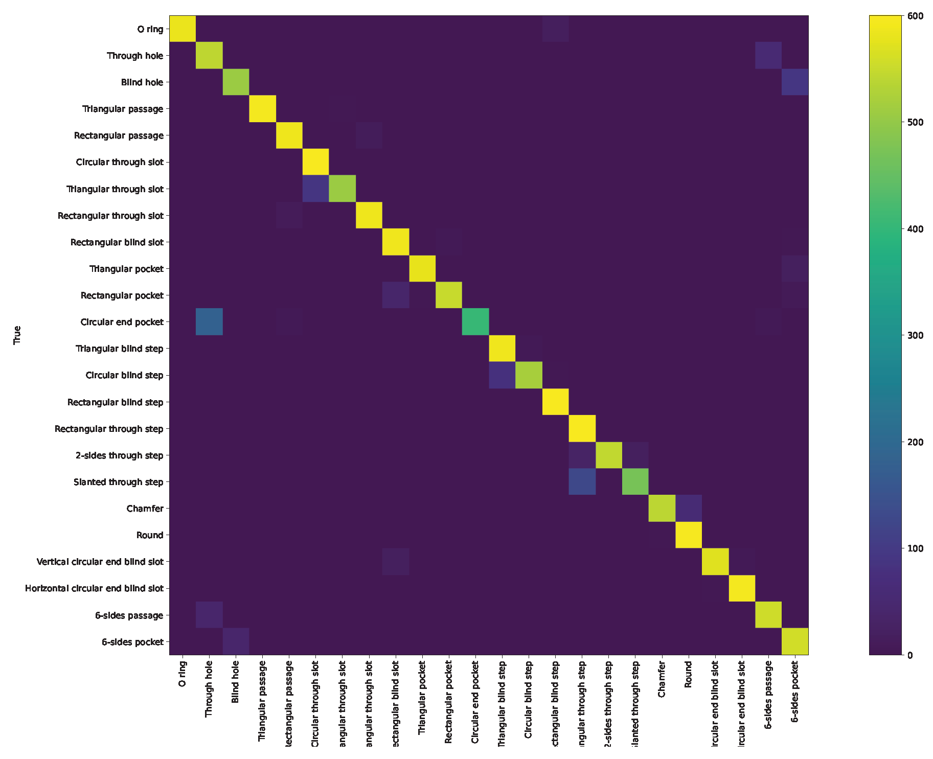
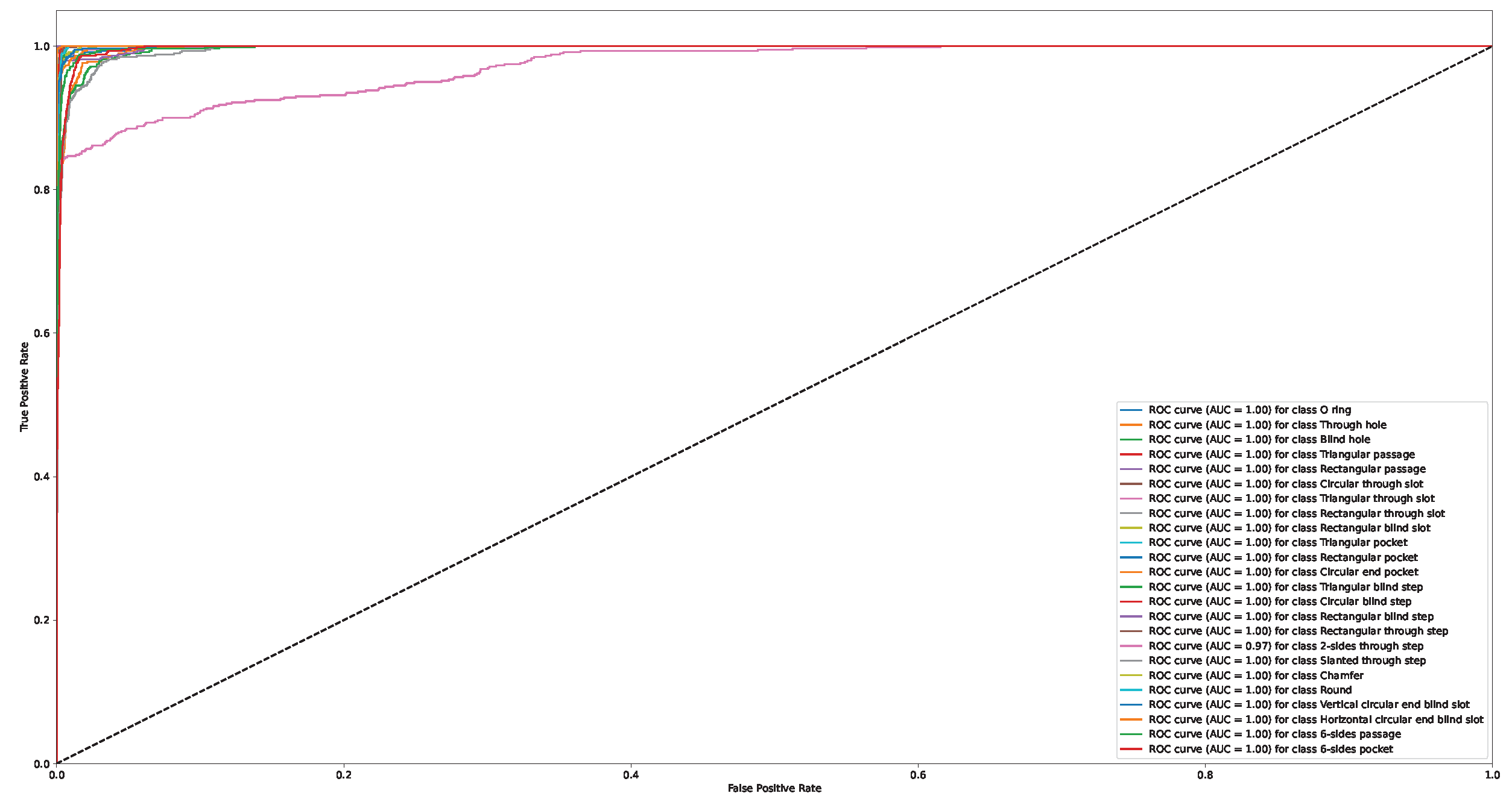
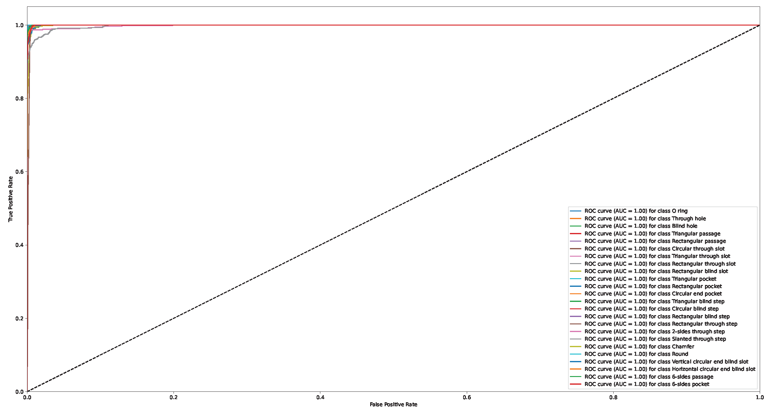
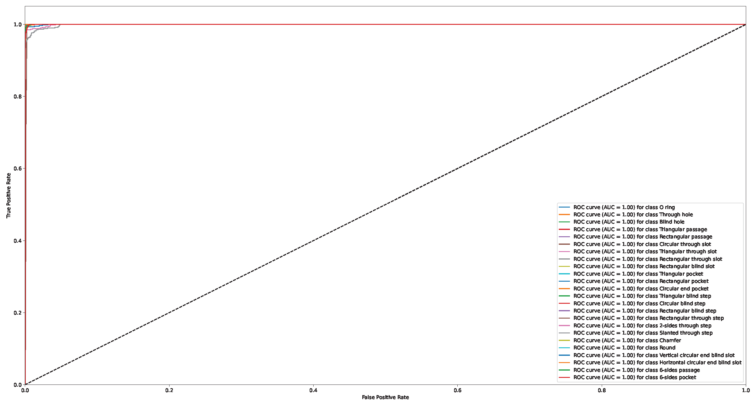
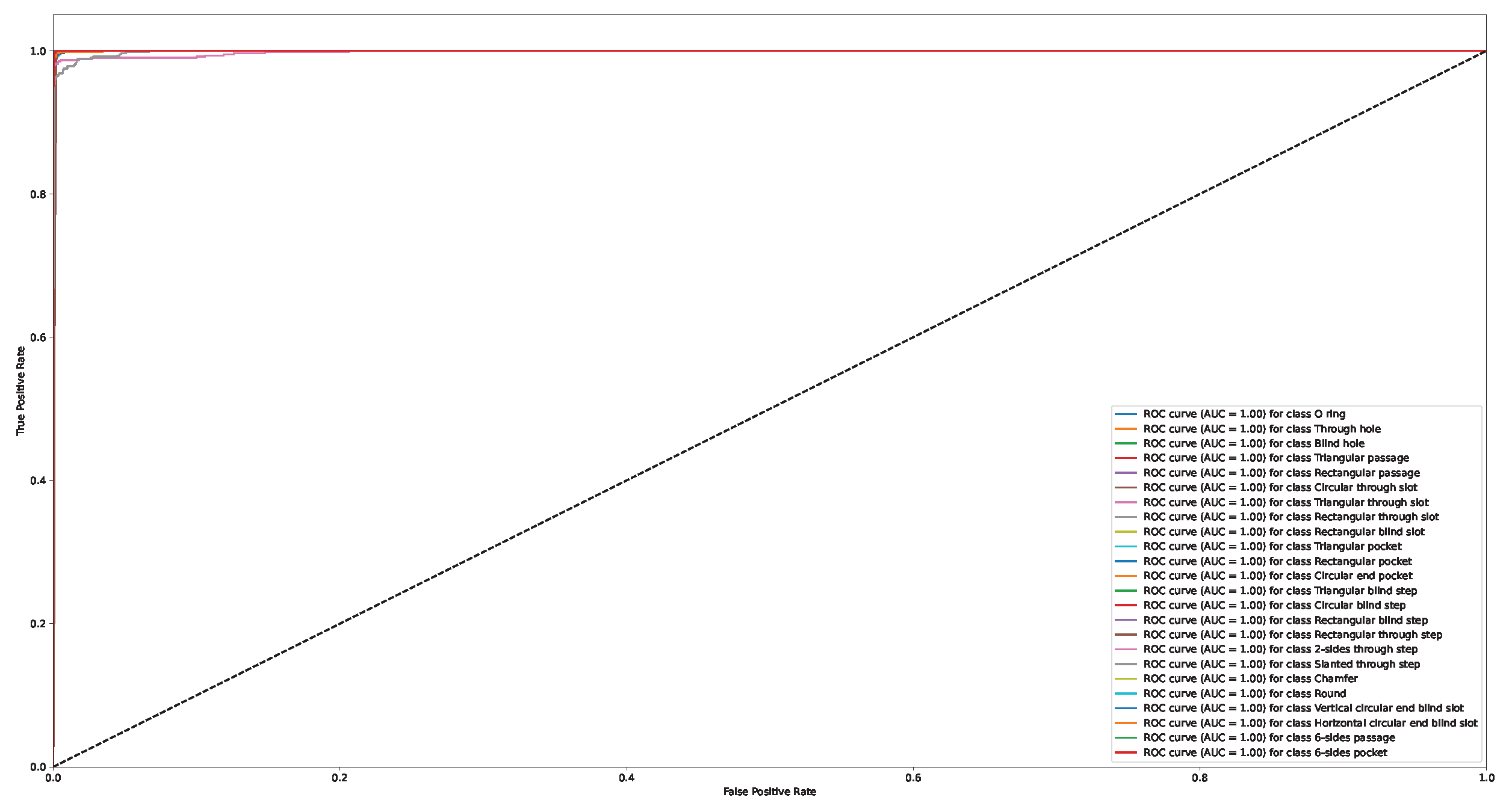
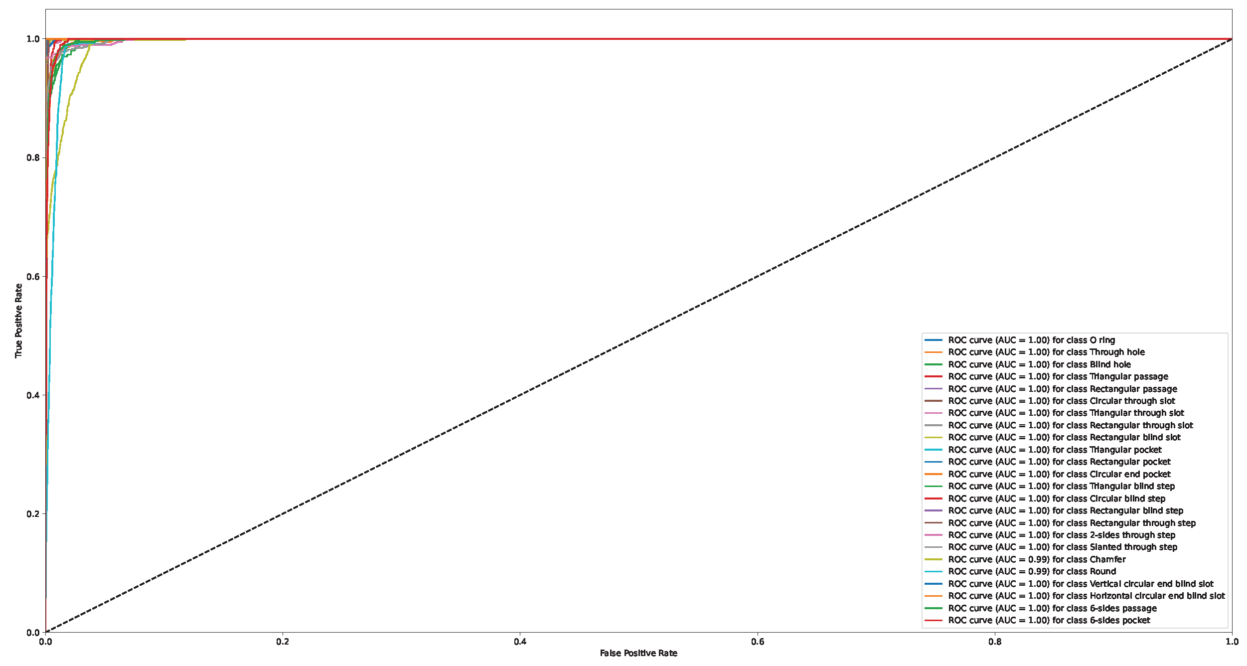
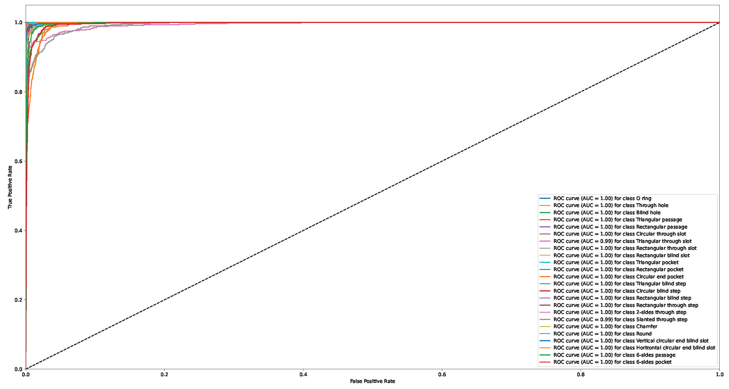
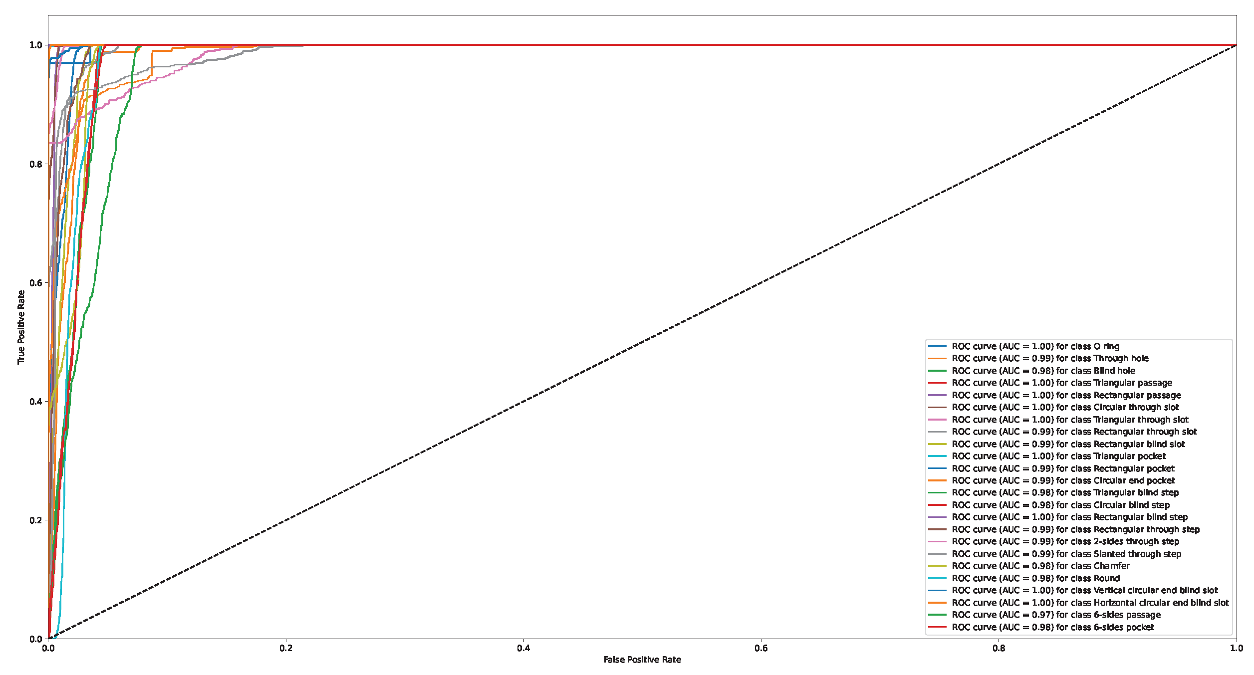
Appendix A. Confusion Matrix and ROC Curve for Different Approaches

Figure A1. Confusion matrix for FeatureNet [14].
Applsci 13 03181 g0a1
Figure A2. Confusion matrix for FeatureNetLite.
Applsci 13 03181 g0a2
Figure A3. Confusion matrix for MsvNet [20].
Applsci 13 03181 g0a3
Figure A4. Confusion matrix for MsvNetLite.
Applsci 13 03181 g0a4
Figure A5. Confusion matrix for [40].
Applsci 13 03181 g0a5
Figure A6. Confusion matrix for [38].
Applsci 13 03181 g0a6
Figure A7. Confusion matrix for VoxNet [59].
Applsci 13 03181 g0a7
Figure A8. ROC curve for FeatureNet [14].
Applsci 13 03181 g0a8
Figure A9. ROC curve for FeatureNetLite.
Applsci 13 03181 g0a9
Figure A10. ROC curve for MsvNet [20].
Applsci 13 03181 g0a10
Figure A11. ROC curve for MsvNetLite.
Applsci 13 03181 g0a11
Figure A12. ROC curve for [40].
Applsci 13 03181 g0a12
Figure A13. ROC curve for [38].
Applsci 13 03181 g0a13
Figure A14. ROC curve for VoxNet [59].
Applsci 13 03181 g0a14

References

  1. Shi, Y.; Zhang, Y.; Xia, K.; Harik, R. A critical review of feature recognition techniques. Comput.-Aided Des. Appl. 2020, 17, 861–899. [Google Scholar] [CrossRef]
  2. Babic, B.; Nesic, N.; Miljkovic, Z. A review of automated feature recognition with rule-based pattern recognition. Comput. Ind. 2008, 59, 321–337. [Google Scholar] [CrossRef]
  3. Vandenbrande, J.H.; Requicha, A.A. Spatial reasoning for the automatic recognition of machinable features in solid models. IEEE Trans. Pattern Anal. Mach. Intell. 1993, 15, 1269–1285. [Google Scholar] [CrossRef]
  4. Nau, D.S.; Gupta, S.K.; Kramer, T.R.; Regli, W.C.; Zhang, G. Development of machining alternatives, based on MRSEVs. In Proceedings of the International Design Engineering Technical Conferences and Computers and Information in Engineering Conference, San Diego, CA, USA, 8–12 August 1993; Volume 97645, pp. 47–57. [Google Scholar] [CrossRef]
  5. Joshi, S.; Chang, T. Graph-based heuristics for recognition of machined features from a 3D solid model. Comput.-Aided Des. 1988, 20, 58–66. [Google Scholar] [CrossRef]
  6. Marefat, M.; Kashyap, R.L. Geometric reasoning for recognition of three-dimensional object features. IEEE Trans. Pattern Anal. Mach. Intell. 1990, 12, 949–965. [Google Scholar] [CrossRef]
  7. Li, Y.; Ding, Y.; Mou, W.; Guo, H. Feature recognition technology for aircraft structural parts based on a holistic attribute adjacency graph. Proc. Inst. Mech. Eng. Part B J. Eng. Manuf. 2010, 224, 271–278. [Google Scholar] [CrossRef]
  8. Kim, Y.S. Volumetric feature recognition using convex decomposition. In Manufacturing Research and Technology; Elsevier: Amsterdam, The Netherlands, 1994; Volume 20, pp. 39–63. [Google Scholar] [CrossRef]
  9. Sakurai, H. Volume decomposition and feature recognition: Part 1—polyhedral objects. Comput.-Aided Des. 1995, 27, 833–843. [Google Scholar] [CrossRef]
  10. Sakurai, H.; Dave, P. Volume decomposition and feature recognition, Part II: Curved objects. Comput.-Aided Des. 1996, 28, 519–537. [Google Scholar] [CrossRef]
  11. Gao, S.; Shah, J. Automatic recognition of interacting machining features based on minimal condition subgraph. Comput.-Aided Des. 1998, 30, 727–739. [Google Scholar] [CrossRef]
  12. Zhang, C.; Chan, K.; Chen, Y. A hybrid method for recognizing feature interactions. Integr. Manuf. Syst. 1998, 9, 120–128. [Google Scholar] [CrossRef]
  13. Henderson, M.R.; Anderson, D.C. Computer recognition and extraction of form features: A CAD/CAM link. Comput. Ind. 1984, 5, 329–339. [Google Scholar] [CrossRef]
  14. Zhang, Z.; Jaiswal, P.; Rai, R. FeatureNet: Machining feature recognition based on 3D Convolution Neural Network. Comput.-Aided Des. 2018, 101, 12–22. [Google Scholar] [CrossRef]
  15. Ning, F.; Shi, Y.; Cai, M.; Xu, W.; Zhang, X. Manufacturing cost estimation based on the machining process and deep-learning method. J. Manuf. Syst. 2020, 56, 11–22. [Google Scholar] [CrossRef]
  16. Prabhakar, S.; Henderson, M.R. Automatic form-feature recognition using neural-network-based techniques on boundary representations of solid models. Comput.-Aided Des. 1992, 24, 381–393. [Google Scholar] [CrossRef]
  17. Ding, L.; Matthews, J. A contemporary study into the application of neural network techniques employed to automate CAD/CAM integration for die manufacture. Comput. Ind. Eng. 2009, 57, 1457–1471. [Google Scholar] [CrossRef] [Green Version]
  18. Shi, P.; Qi, Q.; Qin, Y.; Scott, P.J.; Jiang, X. Highly interacting machining feature recognition via small sample learning. Robot. Comput.-Integr. Manuf. 2022, 73, 102260. [Google Scholar] [CrossRef]
  19. Zhang, H.; Zhang, S.; Zhang, Y.; Liang, J.; Wang, Z. Machining feature recognition based on a novel multi-task deep learning network. Robot. Comput.-Integr. Manuf. 2022, 77, 102369. [Google Scholar] [CrossRef]
  20. Shi, P.; Qi, Q.; Qin, Y.; Scott, P.J.; Jiang, X. A novel learning-based feature recognition method using multiple sectional view representation. J. Intell. Manuf. 2020, 31, 1291–1309. [Google Scholar] [CrossRef] [Green Version]
  21. Chen, X.; He, K. Exploring simple siamese representation learning. In Proceedings of the IEEE/CVF Conference on Computer Vision and Pattern Recognition, Nashville, TN, USA, 20–25 June 2021; pp. 15750–15758. [Google Scholar] [CrossRef]
  22. Zhang, X.; Nassehi, A.; Newman, S.T. Feature recognition from CNC part programs for milling operations. Int. J. Adv. Manuf. Technol. 2014, 70, 397–412. [Google Scholar] [CrossRef]
  23. Xu, T.; Li, J.; Chen, Z. Automatic machining feature recognition based on MBD and process semantics. Comput. Ind. 2022, 142, 103736. [Google Scholar] [CrossRef]
  24. Ferreira, J.; Hinduja, S. Convex hull-based feature-recognition method for 2.5D components. Comput.-Aided Des. 1990, 22, 41–49. [Google Scholar] [CrossRef]
  25. Kim, Y.S.; Wang, E.; Rho, H.M. Geometry-based machining precedence reasoning for feature-based process planning. Int. J. Prod. Res. 2001, 39, 2077–2103. [Google Scholar] [CrossRef]
  26. Woo, Y.; Sakurai, H. Recognition of maximal features by volume decomposition. Comput.-Aided Des. 2002, 34, 195–207. [Google Scholar] [CrossRef]
  27. Woo, Y. Fast cell-based decomposition and applications to solid modeling. Comput.-Aided Des. 2003, 35, 969–977. [Google Scholar] [CrossRef]
  28. Han, J.; Requicha, A.A. Integration of feature based design and feature recognition. Comput.-Aided Des. 1997, 29, 393–403. [Google Scholar] [CrossRef]
  29. Rahmani, K.; Arezoo, B. Boundary analysis and geometric completion for recognition of interacting machining features. Comput.-Aided Des. 2006, 38, 845–856. [Google Scholar] [CrossRef]
  30. Verma, A.K.; Rajotia, S. A hybrid machining Feature Recognition system. Int. J. Manuf. Res. 2009, 4, 343–361. [Google Scholar] [CrossRef]
  31. Yao, X.; Wang, D.; Yu, T.; Luan, C.; Fu, J. A machining feature recognition approach based on hierarchical neural network for multi-feature point cloud models. J. Intell. Manuf. 2022, 1–12. [Google Scholar] [CrossRef]
  32. Shi, P.; Qi, Q.; Qin, Y.; Scott, P.J.; Jiang, X. Intersecting Machining Feature Localization and Recognition via Single Shot Multibox Detector. IEEE Trans. Ind. Inform. 2021, 17, 3292–3302. [Google Scholar] [CrossRef]
  33. Wang, J.; Liu, S. Hopfield neural network-based automatic recognition for 3-D features. In Proceedings of the 1993 International Conference on Neural Networks (IJCNN-93-Nagoya, Japan), Nagoya, Japan, 25–29 October 1993; Volume 3, pp. 2121–2124. [Google Scholar] [CrossRef]
  34. Lankalapalli, K.; Chatterjee, S.; Chang, T. Feature recognition using ART2: A self-organizing neural network. J. Intell. Manuf. 1997, 8, 203–214. [Google Scholar] [CrossRef]
  35. Öztürk, N.; Öztürk, F. Hybrid neural network and genetic algorithm based machining feature recognition. J. Intell. Manuf. 2004, 15, 287–298. [Google Scholar] [CrossRef]
  36. Zhang, Y.; Zhang, S.; Huang, R.; Huang, B.; Yang, L.; Liang, J. A deep learning-based approach for machining process route generation. Int. J. Adv. Manuf. Technol. 2021, 115, 3493–3511. [Google Scholar] [CrossRef]
  37. Ning, F.; Shi, Y.; Cai, M.; Xu, W. Various realization methods of machine-part classification based on deep learning. J. Intell. Manuf. 2020, 31, 2019–2032. [Google Scholar] [CrossRef]
  38. Peddireddy, D.; Fu, X.; Shankar, A.; Wang, H.; Joung, B.G.; Aggarwal, V.; Sutherland, J.W.; Jun, M.B.G. Identifying manufacturability and machining processes using deep 3D convolutional networks. J. Manuf. Process. 2021, 64, 1336–1348. [Google Scholar] [CrossRef]
  39. Mohammadi, N.; Nategh, M.J. Development of a deep learning machining feature recognition network for recognition of four pilot machining features. Int. J. Adv. Manuf. Technol. 2022, 121, 7451–7462. [Google Scholar] [CrossRef]
  40. Ning, F.; Shi, Y.; Cai, M.; Xu, W. Part machining feature recognition based on a deep learning method. J. Intell. Manuf. 2021, 34, 809–821. [Google Scholar] [CrossRef]
  41. Fu, X.; Peddireddy, D.; Aggarwal, V.; Jun, M.B.G. Improved Dexel Representation: A 3D CNN Geometry Descriptor for Manufacturing CAD. IEEE Trans. Ind. Inform. 2021, 9, 5882–5892. [Google Scholar] [CrossRef]
  42. Cao, W.; Robinson, T.; Hua, Y.; Boussuge, F.; Colligan, A.R.; Pan, W. Graph representation of 3d cad models for machining feature recognition with deep learning. In Proceedings of the International Design Engineering Technical Conferences and Computers and Information in Engineering Conference, Boston, MA, USA, 17–19 August 2020; Volume 84003, p. V11AT11A003. [Google Scholar]
  43. Van Engelen, J.E.; Hoos, H.H. A survey on semi-supervised learning. Mach. Learn. 2020, 109, 373–440. [Google Scholar] [CrossRef] [Green Version]
  44. Chen, T.; Kornblith, S.; Norouzi, M.; Hinton, G. A Simple Framework for Contrastive Learning of Visual Representations. In Proceedings of the 37th International Conference on Machine Learning, Vienna, Austria, 12–18 July 2020; Volume 119, pp. 1597–1607. [Google Scholar]
  45. Caron, M.; Misra, I.; Mairal, J.; Goyal, P.; Bojanowski, P.; Joulin, A. Unsupervised learning of visual features by contrasting cluster assignments. Adv. Neural Inf. Process. Syst. 2020, 33, 9912–9924. [Google Scholar]
  46. Grill, J.B.; Strub, F.; Altché, F.; Tallec, C.; Richemond, P.; Buchatskaya, E.; Doersch, C.; Avila Pires, B.; Guo, Z.; Gheshlaghi Azar, M.; et al. Bootstrap Your Own Latent—A New Approach to Self-Supervised Learning. In Proceedings of the Advances in Neural Information Processing Systems, Virtual Event, 6–12 December 2020; Larochelle, H., Ranzato, M., Hadsell, R., Balcan, M., Lin, H., Eds.; Curran Associates, Inc.: Red Hook, NY, USA, 2020; Volume 33, pp. 21271–21284. [Google Scholar]
  47. Zbontar, J.; Jing, L.; Misra, I.; LeCun, Y.; Deny, S. Barlow Twins: Self-Supervised Learning via Redundancy Reduction. In Proceedings of the 38th International Conference on Machine Learning, Virtual Event, 18–24 July 2021; Volume 139, pp. 12310–12320. [Google Scholar]
  48. Sandler, M.; Howard, A.; Zhu, M.; Zhmoginov, A.; Chen, L.C. MobileNetV2: Inverted Residuals and Linear Bottlenecks. In Proceedings of the IEEE Conference on Computer Vision and Pattern Recognition, Salt Lake City, UT, USA, 18–23 June 2018. [Google Scholar]
  49. Howard, A.; Sandler, M.; Chu, G.; Chen, L.C.; Chen, B.; Tan, M.; Wang, W.; Zhu, Y.; Pang, R.; Vasudevan, V.; et al. Searching for MobileNetV3. In Proceedings of the IEEE/CVF International Conference on Computer Vision, Seoul, Korea, 27 October–2 November 2019. [Google Scholar]
  50. Cui, C.; Gao, T.; Wei, S.; Du, Y.; Guo, R.; Dong, S.; Lu, B.; Zhou, Y.; Lv, X.; Liu, Q.; et al. PP-LCNet: A Lightweight CPU Convolutional Neural Network. arXiv 2021, arXiv:2109.15099. [Google Scholar] [CrossRef]
  51. Howard, A.G.; Zhu, M.; Chen, B.; Kalenichenko, D.; Wang, W.; Weyand, T.; Andreetto, M.; Adam, H. MobileNets: Efficient Convolutional Neural Networks for Mobile Vision Applications. arXiv 2017, arXiv:1704.04861. [Google Scholar]
  52. Ye, R.; Liu, F.; Zhang, L. 3D depthwise convolution: Reducing model parameters in 3D vision tasks. In Proceedings of the Canadian Conference on Artificial Intelligence, Kingston, ON, Canada, 28–31 May 2019; pp. 186–199. [Google Scholar]
  53. Ioffe, S.; Szegedy, C. Batch normalization: Accelerating deep network training by reducing internal covariate shift. In Proceedings of the International Conference on Machine Learning, Lille, France, 6–11 July 2015; pp. 448–456. [Google Scholar]
  54. Hu, J.; Shen, L.; Sun, G. Squeeze-and-excitation networks. In Proceedings of the IEEE Conference on Computer Vision and Pattern Recognition, Salt Lake City, UT, USA, 18–22 June 2018; pp. 7132–7141. [Google Scholar]
  55. Simonyan, K.; Zisserman, A. Very Deep Convolutional Networks for Large-Scale Image Recognition. arXiv 2014, arXiv:1409.1556. [Google Scholar]
  56. Su, H.; Maji, S.; Kalogerakis, E.; Learned-Miller, E. Multi-view Convolutional Neural Networks for 3D Shape Recognition. arXiv 2015, arXiv:1505.00880. [Google Scholar] [CrossRef]
  57. Paszke, A.; Gross, S.; Massa, F.; Lerer, A.; Bradbury, J.; Chanan, G.; Killeen, T.; Lin, Z.; Gimelshein, N.; Antiga, L.; et al. Pytorch: An imperative style, high-performance deep learning library. In Proceedings of the Advances in Neural Information Processing Systems 32 (NeurIPS 2019), Vancouver, Canada, 8–14 December 2019. [Google Scholar]
  58. Kingma, D.P.; Ba, J. Adam: A Method for Stochastic Optimization. arXiv 2014, arXiv:1412.6980. [Google Scholar]
  59. Maturana, D.; Scherer, S. VoxNet: A 3D Convolutional Neural Network for real-time object recognition. In Proceedings of the 2015 IEEE/RSJ International Conference on Intelligent Robots and Systems (IROS), Hamburg, Germany, 28 September–3 October 2015; pp. 922–928. [Google Scholar] [CrossRef]
  60. van der Maaten, L.; Hinton, G. Visualizing Data using t-SNE. J. Mach. Learn. Res. 2008, 9, 2579–2605. [Google Scholar]
  61. He, K.; Fan, H.; Wu, Y.; Xie, S.; Girshick, R. Momentum Contrast for Unsupervised Visual Representation Learning. In Proceedings of the IEEE/CVF Conference on Computer Vision and Pattern Recognition (CVPR), Seattle, WA, USA, 13–19 June 2020. [Google Scholar]
  62. Goyal, P.; Dollár, P.; Girshick, R.; Noordhuis, P.; Wesolowski, L.; Kyrola, A.; Tulloch, A.; Jia, Y.; He, K. Accurate, Large Minibatch SGD: Training ImageNet in 1 Hour. arXiv 2017, arXiv:1706.02677. [Google Scholar] [CrossRef]
Figure 1. The pipeline of the proposed semi-supervised machining feature recognition framework.
Applsci 13 03181 g001
Figure 2. The architecture of the self-supervised method.
Applsci 13 03181 g002
Figure 3. The architecture of the three-layer MLP projector.
Applsci 13 03181 g003
Figure 4. The architecture of the two-layer MLP predictor.
Applsci 13 03181 g004
Figure 5. A detailed view of FeatureNetLite; k = 3 denotes convolution kernel size is set to 3.
Applsci 13 03181 g005
Figure 6. The difference between the DSConv3D block and a standard 3D convolution block.
Applsci 13 03181 g006
Figure 7. A detailed view of MsvNetLite.
Applsci 13 03181 g007
Figure 8. Machining features in the FeatureNet dataset [14].
Applsci 13 03181 g008
Figure 9. The t-SNE visualization of the visual representation on test set: (a) the backbone output of MsvNetLite after fine-tuning using the SGDM optimizer in semi-supervised learning, (b) the backbone output of MsvNetLite initialized with ImageNet pre-trained weights, (c) the backbone output of MsvNetLite with random initialization, (d) the backbone output of MsvNetLite after the self-supervised stage in semi-supervised learning, (e) the backbone output of MsvNetLite after supervised learning, (f) the backbone output of MsvNetLite after fine-tuning using the Adam optimizer in semi-supervised learning.
Applsci 13 03181 g009
Table 1. Configuration details of FeatureNetLite; k = 3 denotes that convolution kernel size is set to 3, and S E denotes whether to use the Squeeze-and-Excite module. And if S E is set to ✓, it means Squeeze-and-Excite module is enabled.
OperatorSEStrideInput ( C × H × W × D )Output ( C × H × W × D )
Stem Conv3D, k = 3-2 1 × 64 3 16 × 32 3
DSConv3D, k = 3-1 16 × 32 3 32 × 32 3
DSConv3D, k = 3-2 32 × 32 3 64 × 16 3
DSConv3D, k = 3-1 64 × 16 3 64 × 16 3
DSConv3D, k = 3-2 64 × 16 3 128 × 8 3
DSConv3D, k = 3-1 128 × 8 3 128 × 8 3
DSConv3D, k = 3-2 128 × 8 3 256 × 4 3
5× DSConv3D, k = 5-1 256 × 4 3 256 × 4 3
DSConv3D, k = 52 256 × 4 3 512 × 2 3
DSConv3D, k = 51 512 × 2 3 512 × 2 3
GAP3D-- 512 × 2 3 512 × 1 3
Conv3D, k = 1-1 512 × 1 3 1280 × 1 3
Flatten-- 1280 × 1 3 1280
Linear--128024
Table 2. Configuration details of MsvNetLite; k = 3 denotes convolution kernel size is set to 3, and S E denotes whether to use the Squeeze-and-Excite module. And if S E is set to ✓, it means Squeeze-and-Excite module is enabled.
OperatorSEStrideInput ( V × C × H × W )Output ( V × C × H × W )
Stem Conv2D, k = 3-2 12 × 3 × 64 2 12 × 16 × 32 2
DSConv2D, k = 3-1 12 × 16 × 32 2 12 × 32 × 32 2
DSConv2D, k = 3-2 12 × 32 × 32 2 12 × 64 × 16 2
DSConv2D, k = 3-1 12 × 64 × 16 2 12 × 64 × 16 2
DSConv2D, k = 3-2 12 × 64 × 16 2 12 × 128 × 8 2
DSConv2D, k = 3-1 12 × 128 × 8 2 12 × 128 × 8 2
DSConv2D, k = 3-2 12 × 128 × 8 2 12 × 256 × 4 2
5× DSConv2D, k = 5-1 12 × 256 × 4 2 12 × 256 × 4 2
DSConv2D, k = 52 12 × 256 × 4 2 12 × 512 × 2 2
DSConv2D, k = 51 12 × 512 × 2 2 12 × 512 × 2 2
View pooling-- 12 × 512 × 2 2 512 × 2 2
GAP2D-- 512 × 2 2 512 × 1 2
Conv2D, k = 1-1 512 × 1 2 1280 × 1 2
Flatten-- 1280 × 1 2 1280
Linear--128024
Table 3. The recognition accuracy (%) of several approaches on the FeatureNet test dataset: P T denotes pre-trained weights, D A denotes data augmentation, and Semi-Sup. denotes semi-supervised learning. The bold number is the best result in each column.
ApproachData
Format
Training
Strategy
Number of
Training Data per Class
PTDASemi-Sup.1248163264128
 [20]Multi-view 13.4217.8522.8835.4452.9367.1587.6594.47
28.8848.5260.5173.0384.8892.3896.1298.03
16.7726.7247.7265.6082.3392.6796.6498.65
50.3473.1786.6592.7194.5197.2398.5499.01
MsvNetLite (ours) 6.037.589.6715.1226.3348.7468.5685.52
25.8135.1047.5267.5882.3294.6995.8898.31
13.9918.2234.1656.9771.3886.3694.0695.70
45.2357.0081.0389.2494.7097.0798.4198.76
69.8176.0487.7493.9597.1597.5698.0398.84
 [14]Voxel 12.7014.4215.7818.8727.9030.5843.3152.28
16.6718.6824.0842.4259.2475.0290.7394.26
FeatureNetLite (ours) 4.175.639.0812.3515.2322.6338.7969.17
8.7816.0523.8544.5367.9283.0790.6094.65
36.5256.4061.0074.4286.5391.8392.1297.10
 [38] 11.1711.7617.5921.3825.7432.6041.6555.36
15.4720.3128.6245.7360.9876.8886.7994.34
 [40] 8.0510.8614.6920.8127.2831.1838.3554.16
14.9719.4220.3235.6757.9067.4783.7893.38
 [59] 10.2213.4416.9717.7022.3229.5638.6048.90
15.2218.9724.8431.2445.8361.2569.7077.74
Table 4. The comparison of optimal recognition accuracy (%), network size, and average inference latency with different approaches. The bold number is the best result in each column.
NetworkOptimal Accuracy (%) ↑ParametersFLOPsLatency (ms) @
GPU ↓
Latency (ms) @
CPU ↓
 [20]99.01128.86 M7.46 G8.83127.89
MsvNetLite (ours)98.841.70 M0.16 G6.9619.27
 [14]94.2633.94 M12.51 G13.36137.88
FeatureNetLite (ours)97.101.91 M0.14 G6.9055.97
 [38]94.3433.75 M6.40 G7.6071.28
 [40]93.3832.75 M10.70 G15.43178.72
 [59]77.7411.27 M0.73 G1.7420.31
Table 5. The test accuracy (%) of the MsvNetLite with different numbers of unlabeled data per class in the self-supervised stage. The bold number is the best result in each column.
Number of Unlabeled Data per Class
in Self-Supervised Stage
Number of Labeled Data per Class for Fine-Tuning
1248163264128
360051.7864.2277.6086.1792.1294.9297.0498.28
600069.8176.0487.7493.9597.1597.5698.0398.84
Table 6. The test accuracy (%) of the MsvNetLite with different batch sizes in the self-supervised stage. The bold number is the best result in each column. The bold number is the best result in each column.
Batch Size in Self-Supervised StageNumber of Labeled Data per Class for Fine-Tuning
1248163264128
1664.0874.7683.9092.2595.2696.8298.1298.63
3269.8176.0487.7493.9597.1597.5698.0398.84
6431.4048.9559.1875.2884.6392.2894.6997.14
12825.2644.2145.2870.6772.7983.8890.4695.60
25653.6768.9983.3392.8195.4096.8397.9498.56
Table 7. The test accuracy (%) of the MsvNetLite with different training epochs for self-supervised learning. The bold number is the best result in each column.
Training Epoch in Self-Supervised StageNumber of Labeled Data per Class for Fine-Tuning
1248163264128
5053.4463.7866.0274.2483.8393.8197.2897.62
10069.8176.0487.7493.9597.1597.5698.0398.84
20076.3386.9487.3092.5294.5496.6597.2598.38
Table 8. The test accuracy (%) of the MsvNetLite with different data augmentation strategies in the self-supervised stage. The denotes this augmentation method is enabled. The bold number is the best result in each column.
Data Augmentation Strategies
in Self-Supervised Learning Stage
Number of Labeled Data per Class for Fine-Tuning
RotationScalePadCrop1248163264128
22.2831.3343.6652.2673.0674.3584.3196.18
34.4143.5161.5571.5884.4491.9994.8496.94
69.8176.0487.7493.9597.1597.5698.0398.84
Table 9. The recognition accuracy (%) of the MsvNetLite with different optimizers for fine-tuning. The bold number is the best result in each column.
Optimizer for Fine-TuningNumber of Labeled Data per Class for Fine-Tuning
1248163264128
Adam15.3921.6213.2124.0826.4281.9994.9396.15
SGDM ( m o m e n t u m = 0.9 )69.8176.0487.7493.9597.1597.5698.0398.84
SGD66.9873.8582.0883.7093.8396.2497.9998.53
RMSProp7.717.179.198.1710.2444.9780.1289.21
Disclaimer/Publisher’s Note: The statements, opinions and data contained in all publications are solely those of the individual author(s) and contributor(s) and not of MDPI and/or the editor(s). MDPI and/or the editor(s) disclaim responsibility for any injury to people or property resulting from any ideas, methods, instructions or products referred to in the content.

