1. Introduction
Nowadays, as a risk-eliminating and cost-saving tool, unmanned surface vehicles (USVs) [
1] play an important role in maritime applications. Meanwhile, in inland marine environment, more and more activities such as hydrologic surveys, harbor surveillance, maritime search and rescue, have witnessed their prevailing success. In general, the USVs are equipped with a variety of sensors (i.e., sensing devices) to capture significant environmental information around them and guide their following correct movements. As an indispensable optical sensor, an ordinary digital camera has been popular for USVs due to its benefits of usage and economy. Among the vision information obtained by this type of sensor, the waterline is one of the most important visual cues for USVs, since it is usually treated as a reference target of sailing to facilitate USVs to carry out numerous critical missions. For example, based on computer vision techniques, the USVs mounted with a camera sensor can accomplish obstacle avoidance and autonomous navigation through recognizing the sailing area from captured optical images. Accordingly, effectively identifying waterlines in images, namely vision-based waterline detection, has been desired to assist USVs to perform anticipated actions including ensuring their own sailing security. However, it is challenging for USVs with camera sensors to achieve satisfactory detection effects within inland water, because of the visual complexity of inland waterlines, such as their own irregularity and versatility, as well as the diversity and dynamics of their surroundings.
With the development of computer vision techniques, many waterline detection approaches by virtue of a general digital camera have been proposed. Most of them aim at the detection of coastal waterline in sea areas, e.g., [
2,
3,
4,
5], and there are also a few works focusing on inland waterline, e.g., [
6,
7,
8]. When applied in inland waters, the detection effects of these approaches tend to be vulnerable to the variations of environmental factors (e.g., weather conditions such as fog, snow or rain, illumination conditions such as shadow, reflection or water glint, the shapes of waterlines, as well as the viewpoints of cameras). The reason is that the erratic environmental factors usually engender more visual complexity on the inland waterline. For example, the visual information of the background surrounding an inland waterline might become more confusing due to the change of illumination. Correspondingly, the stability of existing approaches is prone to be disturbed in such changeable and complicated inland water scenarios.
Specifically, existing vision-based waterline detection approaches generally share a pipeline that consists of two relevant processes, i.e., waterline-relevant feature representation and discriminative strategy (or algorithm) for final identification, respectively. For instance, some approaches [
4,
9,
10] considered waterline detection as an issue on edge detection, wherein they firstly extracted the features pertinent to edge (or line) according to specific prior knowledge or statistical assumptions, and then identified the edge (or line) capable of approximately fitting the waterline within an image via a discriminative strategy determined in advance or algorithm associated with the previously represented features. Moreover, there are a number of other vision-based approaches that treat waterline detection as an image segmentation task [
11,
12]. They similarly followed the pipeline comprising feature representation and discriminative strategy. Nevertheless, current proposals for the two relevant processes in these vision-based approaches tend to overwhelm the stability of the approaches themselves, due to their deficiencies in the robustness against variable inland water environments. The deficiencies of the proposals are summarized as follows:
- (i)
The current proposals for representing waterline-relevant features are hand-crafted that largely depend on specific prior knowledge or statistical assumptions, whereas the applied prior knowledge or assumptions cannot hold in all cases. For example, the waterline was viewed as a horizon line in [
4,
13]. Despite the prior knowledge facilitates representing the features relating to the water-sky-line, it is not always correct in other waterline detection tasks, e.g., water-land-line detection in inland waters. As another example, some studies [
14,
15] resorted to classical edge detection algorithms for waterline detection. Similar to conventional feature representation for edges, their means of representing waterline-relevant features usually built on statistical assumptions related to image gradient information, such as classic Canny operators [
16]. Although they rendered satisfactory results in real-world tasks, the waterline-relevant features represented in this way are sensitive to noise brought about by the variations of environmental factors. Thus, the discriminative ability of the waterline-relevant features is limited to their applicable scenarios. In addition, before applying the proposals to extract waterline-relevant features, the original images obtained by the USVs generally need to be preprocessed, e.g., image enhancement or denoising, which might impact the efficiency of waterline detection in USVs more or less.
- (ii)
The currently used discriminative strategies (or algorithms) to finalize waterline identification mostly work in particular water conditions, which have little consideration for coping with the visual versatility of waterline caused by the variations of environmental factors. For example, in [
17], albeit the researchers devised a sophisticated approach to represent waterline-relevant features via classical image structure and texture analysis after image preprocessing, their proposed discriminative strategy is relatively simple and rigid. Specifically, they utilized an empirical value as the threshold of image segmentation to finally discriminate the waterline. Similarly, ref. [
6] used an improved maximum or minimum gradient value sample method as the tenacious selecting rule of waterline candidate pixels. Regarding the discriminative strategies (or algorithms) built on the previously extracted waterline-relevant features, as water environments are varying, their ability to identify a waterline might be degraded or even fail. Hence, the discriminative strategies (or algorithms) are inflexible, which cannot be broadly applicable to varied inland water environments simultaneously.
With the motivation of tackling the above deficiencies, this paper aims to guarantee the effectiveness of waterline detection for the USVs with an ordinary digital camera in variable inland water environments via machine learning techniques. To achieve this, we make an attempt to improve the robustness and stability of waterline detection for diverse cases by proposing a general deep-learning-based paradigm for inland marine USVs, named DeepWL, which concerns the efficiency of waterline detection simultaneously. As illustrated in
Figure 1, the proposed paradigm consists of two cooperative deep neural network models. One, termed WLdetectNet, is customized as the primary network (i.e., a learning model) for our deep visual waterline detection by exploiting convolutional neural networks (CNNs) [
18]. The other one, named WLgenerateNet, is built upon generative adversarial networks (GANs) [
19] that serves as the auxiliary network (i.e., another learning model) of WLdetectNet.
As the mainstay of this paradigm, the WLdetectNet is modeled as an end-to-end deep convolutional neural network to directly achieve the identification of candidate waterlines in each image captured by USVs, rather than separating waterline-relevant feature representation from its related discriminative strategy (or algorithm), and without resorting to image preprocessing. To improve the accuracy of waterline detection, we innovatively devise two significant schemes (presented in
Section 3.1) for the materialization of WLdetectNet by following the same architectural principles with many modern deep CNNs (e.g., MobileNet [
20] and ResNet [
21]), which are actually dedicated to the improvement of the representational capability of this deep learning model for varied waterlines. At the same time, owing to its architectural characteristics benefiting from the two specialized schemes, WLdetectNet lays stress on the efficiency of waterline detection as well. What is more, to improve the robustness of WLdetectNet for variable inland water environments, another deep neural network, i.e., WLgenerateNet, is built to assist the improvement of the generalization ability of WLdetectNet in diverse cases by exploiting the classical generative adversarial networks, such as DCGAN [
22]. In brief, the overall design for the proposed paradigm is inspired by the current great successes of deep learning techniques in computer vision applications, especially the modern CNNs for object detection [
23] and the classical GANs for image generation [
24].
To summarize, the main contributions of this paper are as follows. First, we model the challenging issue on the visual detection of a waterline as an end-to-end machine learning task based on deep neural networks by proposing an alternative waterline detection paradigm (DeepWL) for inland marine USVs, which makes the waterline-related feature representation and its subsequent waterline discrimination automatically work together in one unified deep network model (WLdetectNet) without any priors or assumptions, and simultaneously achieves their robustness and stability for diverse cases in complicated inland waters via a scalable and generalizable training set constructed by another deep network model (WLgenerateNet). Second, based on the proposed paradigm, we present an algorithm to conduct waterline image-map estimation from video frames captured on board, which formulates the learning task on vision-based waterline detection as a sequence of repetitive subtasks on distinguishing the segments relevant to a waterline (i.e., waterline segments). Importantly, to ensure the effectiveness and efficiency of our waterline detection algorithm, we propose two significant schemes to implement the mainstay of this paradigm (i.e., WLdetectNet): one of them concentrates on the visual perception ability of the deep network, and the other scheme aims to bolster the representational capability of the deep network with little extra computational cost. Finally, we define relevant metrics specialized for the quantitative evaluation of the visual waterline detection approach on related performances, and then conduct empirical investigations on the effectiveness and superiority of the proposed approach via qualitative and quantitative assessment. Compared with other alternative approaches, the proposed approach achieves better robustness and stability in the presence of environmental noises in variable inland water. Moreover, we explain the success of the proposed approach for the vision-based waterline detection task in such scenarios from the perspective of visualization, and discuss its case study as well.
The remainder of this paper is organized as follows.
Section 2 introduces the related work on vision-based waterline detection and architecture of deep neural networks. The details of the proposed approach are presented in
Section 3. Experimental results and evaluation are illustrated in
Section 4, followed by the discussion in
Section 5.
Section 6 concludes the paper.
3. Methodology
In order to guarantee the effectiveness of waterline detection for the USVs mounted with a general digital camera sailing in varied inland water environments, especially concerning their accuracy and robustness, we propose a deep-learning-based paradigm termed DeepWL, which also cares about the efficiency of waterline detection for the inland USVs. As illustrated in
Figure 1, the paradigm comprises two collaborative deep neural networks, in which the above one, termed WLdetectNet, is devised as the mainstay of this paradigm that acts as the main network of carrying out the task on vision-based waterline detection, and the other one below, termed WLgenerateNet, serves as the auxiliary network of WLdetectNet. Thus, in this section, we first highlight the architectural details of the two significant deep networks, and then describe their training methods. Finally, based on the proposed paradigm, we present an algorithm to achieve waterline detection.
3.1. The Main Network WLdetectNet
In this paradigm, we specify the vision-based waterline detection as an end-to-end binary classification model, which integrates the waterline-relevant feature representation and its subsequent waterline discriminator in a customized deep convolutional neural network, i.e., WLdetectNet. To improve the accuracy of waterline detection, we deliberately devise the following two specialized schemes to construct the deep model.
3.1.1. Building a Perceptive Block as the Receptive Field of WLdetectNet
Given the visual complexity of waterline in varied inland water environments, we intentionally build a block to specialize in perceiving the contextual information relevant to waterline segments, and make use of the perceptive block as the receptive field of WLdetectNet, i.e., as the first layer of the deep main network in our paradigm DeepWL. As shown in
Figure 2, the premeditated block, termed WLpeephole, is designated to be an image region of size
, which consists of two different size fields (i.e.,
and
, besides
). Specifically, in order to more conveniently and precisely distinguish various segments relevant to a waterline, i.e., waterline segments, we take advantage of two different scale squares with the same central point, called observing field (
) and recognizing field (
), respectively, and further mandate the candidate segments of the waterline to emerge only in the smaller square (i.e.,
recognizing field). Correspondingly, the area between the
observing field and the
recognizing field, namely the area
observing field surrounding the
recognizing field, may be filled with various contextual information associated with a waterline segment, e.g., water streak, plants or buildings at the waterfront.
Intuitively, the special design on the block can draw visual attention to the waterline within a receptive field. In practice, by feeding an image patch in accordance with the block-based design into our deep network WLdetectNet, we can get hold of the more discriminative waterline feature that avails final accurate decision-making on whether this image patch contains a waterline or not. The reason is that the block based on the design carries better characteristics for making distinctions between waterline and non-waterline by paying attention to necessary contexts associated with a waterline in such a receptive field. In addition, the disparity information mingled in a block facilitates WLdetectNet (whose architecture is specified in
Table 1) to bolster the ability of the deep network regarding waterline-relevant feature representation, which will be also interpreted further in
Section 5. Moreover, in our waterline detection algorithm (presented in
Section 3.4), the perceptive block WLpeephole actually behaves as a peephole that successively diagnoses each region across an image captured by USVs to tell whether the current diagnosed region (i.e., current receptive field of WLdetectNet) contains a waterline or not.
3.1.2. Deepening WLdetectNet to Improve Its Own Representational Capability
It is generally believed that improving their own representational capability of learning models is a predominant means to bolster the specific performance of tasks based on machine learning, such as accuracy on prediction. As a prosperous deep learning model, CNNs have been extensively applied in a variety of computer vision tasks including object detection [
31,
32]. In addition, numerous current research works on CNNs [
33,
34,
35] have demonstrated that extending the depth of this deep learning model, namely increasing the number of network layers, is the most straightforward way to improve its representational power. The reason is that the deeper neural networks usually can fit more complicated nonlinear mapping from inputs to outputs that indicates the more robust representational power corresponding to the deep networks. Accordingly, to bolster some particular performances of learning tasks, many prominent variants of the basic deep neural networks have been proposed in this way, such as ResNet [
21] for accurate image classification, and DeeptransMap [
36] for robust single image dehazing.
Inspired by the great success of extending the depth of CNNs, in this paper, we innovatively constitute a rather deep architecture for WLdetectNet to guarantee its robust representational capability, thus improving the accuracy of the main network for waterline detection. A complete description of its architectural specification is presented in
Table 1. It is worth mentioning that, similar to many modern variants of CNNs, some critical architectural principles are adopted in the construction of the deep network. For example, to extend the depth of WLdetectNet, we repeatedly exploit several structural modules in the residual branch of WLdetectNet such as ResNet [
21]. Then, to facilitate training such a deep network, we similarly take advantage of the shortcut path to back-propagate gradients. Meanwhile, in order to alleviate the information loss in such a deep network as much as possible to ensure the effectiveness and efficiency of this deep network in diverse cases, within each of the repeated structural modules, we attempt to successively make use of pointwise group convolution (i.e., PGconv [
28]), channel shuffle operation (i.e., Shuffle [
28]), depthwise convolution (i.e., Dwconv [
20]), point convolution (i.e., Pconv [
20]), global average pooling (i.e., GAP), fully connected operations (i.e., FC, with a Relu and Sigmoid activation, respectively) and channel-wise scaling operation (i.e., Scale [
35]) to enrich and equalize the information flow in the main network of our proposed paradigm. Especially, the reasonable utilization of PGconv [
28] and Dwconv [
20] in our architectural design of WLdetectNet benefits reducing the number of network parameters and computational complexity, which are crucial for guaranteeing the efficiency of the deep network. Actually, despite being deepened, WLdetectNet has little extra computational cost, about 3.12 MFLOPs (i.e., the number of floating-point multiplication-adds) which is very suitable for the inland USVs with computationally limited application. In addition, the channel operation Shuffle [
28] adopted in our architectural design also contributes to ensure the robust representational capability of WLdetectNet by equalizing the information flow in such a deep network.
As shown in
Table 1, WLdetectNet uses an individual image region perceived in accordance with WLpeephole as its input (i.e., the first layer of the deep network), and at its last layer outputs a scalar value indicating the category of the corresponding region, namely waterline or non-waterline. Moreover, apart from its input and output, the overall architecture of WLdetectNet is a linear stack of five repeatable structural modules, which totally consists of 72 convolutional layers. Because of following the common architectural principles of modern deep CNNs such as ResNet [
21], WLdetectNet is easy to be constructed and trained.
3.2. The Auxiliary Network WLgenerateNet
To guarantee the stability of our waterline detection approach under varied inland water environments (i.e., its robustness), in the proposed paradigm DeepWL, we intentionally arrange another deep network named WLgenerateNet as an auxiliary network to assist the main network WLdetectNet in improving its generalization ability. Moreover, the accuracy and efficiency of WLdetectNet continue to be maintained. Specifically, we construct the WLgenerateNet by following the design principles of GANs [
19], and then utilize it to build on demand a large amount of waterline samples relevant to various scenarios for training WLdetectNet, thus generalizing the representational capability of the WLdetectNet and enabling the main network of our paradigm to be effectively applicable for waterline detection in diverse scenarios. That is motivated by a fact in machine learning: more data samples help to improve the generalization ability of a model (e.g., CNNs) and mitigate its problem of overfitting, thus improving the robustness of the model. However, it is actually not easy to collect such a large amount of labeled data on various waterlines. Therefore, in our waterline detection approach, we ingeniously draw lessons from the spirit of GANs that they can enable the automatic generation of desired data.
Similar to classic GANs such as DCGAN [
22], the WLgenerateNet consists of two convolutional neural networks contesting with each other in a zero-sum game framework, where the two adversarial networks are a generator
G(z) for generating waterline samples and a discriminator
D(x) for discriminating waterline samples, respectively.
Table 2 illustrates its architecture.
In the WLgenerateNet, we utilize a 100-dimensional random noise z as its input, then convert z into a 64 × 64 pixel image x by generator . Meanwhile, discriminator is applied to determine whether the currently generated image x belongs to a waterline. Just in the case that the result of is true, the WLgenerateNet outputs generated images. Finally, through an iterative process of and contesting with each other, we can gain our desired labeled data on waterlines.
3.3. Training Methods of Two Deep Networks
As illustrated above, the proposed paradigm DeepWL comprises two specially designed deep neural networks, i.e., WLdetectNet and WLgenerateNet. In addition, their architectures have been presented in
Section 3.1 and
Section 3.2, respectively. Thus, in this section, we focus on their training methods, in which the WLdetectNet is trained in a supervised learning fashion while the WLgenerateNet is trained in an unsupervised learning fashion.
3.3.1. Training WLdetectNet by Supervised Learning
The WLdetectNet acts as the mainstay of DeepWL. According to its design schemes described previously, WLdetectNet aims to capture discriminative information relevant to waterline segments for final waterline detection. Thereby, in order to guarantee its accuracy and generalization ability, a large amount of training data is required, except for those significant designs regarding its architecture (described in
Section 3.1). However, no public dataset on waterlines is available at present. Moreover, as mentioned before, it is also very difficult to collect such a large dataset, due to the labor and economic costs. To effectively carry out the training of WLdetectNet, we opt to build our own dataset on waterline segments in a simple and economical manner, which involves the following two processes.
- (1)
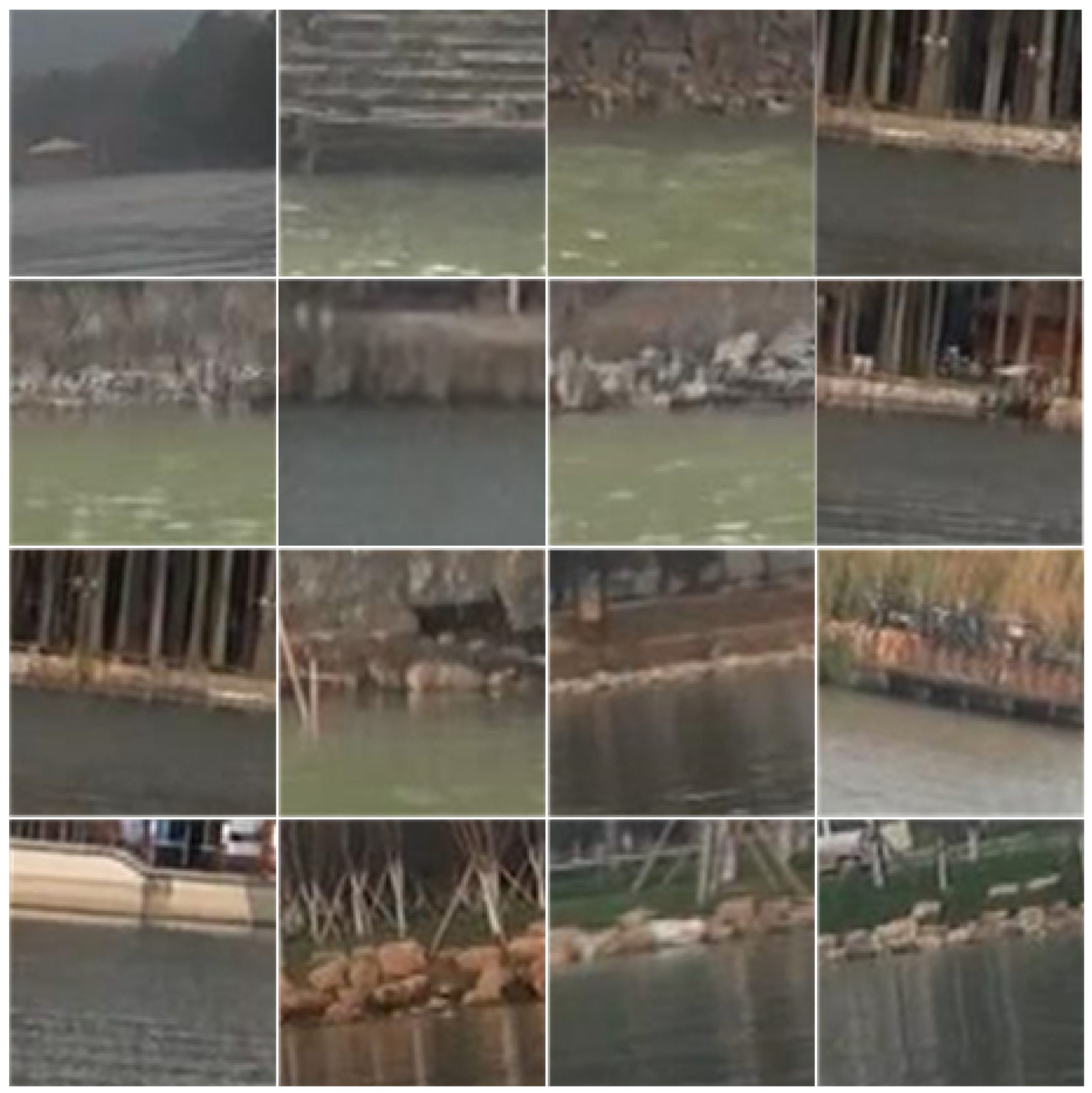
Manually gathering original data satisfying the structural layout of WLpeephole
We first gather 2000 image patches containing diverse waterline segments by manually cropping from surveillance videos associated with an inland waterline, then resize them to be consistent with the structural layout of WLpeephole, especially compelling their waterline segments to display only in a smaller scope identical to the recognizing field
of WLpeephole.
Figure 3 shows such a group of exemplars including 16 image patches. In practice, these gathered image patches come from varied scenarios including dissimilar weather conditions and different illumination conditions, so that the diversity of these samples is helpful for enhancing the perceptive ability of WLpeephole to detect various waterline segments, thus improving the generalization ability of WLdetectNet.
- (2)
Automatically generating artificial data on waterline segments for data augmentation
It is common knowledge that one of the best ways to improve the performance of a deep learning model is to add more data to its training set. However, due to labor and economical costs, it has been proved to not be an easy thing to hunt for plentiful labeled data on waterline segments. Thus, aside from manually gathering more such samples that are representative of distinct waterline segments, we also attempt to augment the labeled data we already have by means of WLgenerateNet. Specifically, we make advantage of WLgenerateNet to automatically generate more artificial data on waterline segments (almost 8000 image patches at present) from the existing manual dataset (i.e., 2000 image patches). In fact, our approach to data augmentation by GANs on images is great for combating overfitting that is one of the primary problems with machine learning models in general, since we can further enlarge these data on demand.
Figure 4 shows two groups of distinct instances generated by WLgenerateNet corresponding to the exemplars in
Figure 3.
Through the above two processes of manually gathering and automatically generating, around 10,000 image patches on waterline segments have constituted the positive samples of our training set. Furthermore, the training set also contains about 12,000 negative samples that are freely cropped from various non-waterline images. Importantly, the training set is a scalable and generalizable dataset, since it can further generalize and augment its sample data according to the needs of practical applications by the two processes mentioned above.
Then, based on the built dataset, we conduct the training for WLdetectNet by minimizing an energy function, which can be formally expressed as:
where
N is the number of training samples,
refers to all parameters of the deep learning model WLdetectNet,
denotes the
training sample,
denotes the output of WLdetectNet over
whose architecture is described in
Table 1, and
represents the ground-truth label of sample
with scalar-valued 1 for waterline and 0 for non-waterline. Our optimization goal for this energy function is to chase the sweet spot where the cross-entropy loss of WLdetectNet is low when its parameters are tuned by stochastic gradient descent (SGD) with a batch size of 60. Moreover, to avoid gradient explosions, our training procedure for WLdetectNet is divided into two stages: we first employ the samples gathered manually and 3000 negative cases to train WLdetectNet for 30 epochs, then apply the data generated by WLgenerateNet and 9000 negative cases to fine-tune WLdetectNet for 50 epochs. Finally, a binary classification deep network to detect waterline segments based on WLpeephole is obtained.
3.3.2. Training WLgenerateNet by Unsupervised Learning
As an auxiliary facility in DeepWL, WLgenerateNet aims to support the generalization ability of another deep learning model WLdetectNet by rendering more training data as much as possible for WLdetectNet. Similar to other classic GANs, its learning objective corresponds to a minmax two-player game, which is formulated as:
where the generator
is responsible for learning to map data
z from the noise distribution
to the distribution
over data
x, while the discriminator
answers for estimating the probability of a sample from the data distribution
rather from
.
Our training for WLgenerateNet is built on the 2000 positive samples gathered by hand with a batch size of 16. All parameters of this deep learning model are initialized from a zero-centered normal distribution with a standard deviation of 0.02. For the activation function LeakyReLU, the slope is set to 0.2. Moreover, the whole training procedure involves two concurrent stages: we maximize
for
, and simultaneously minimize
for
by applying the Adam [
37] optimizer with a momentum of 0.9. During the training, we first use a learning rate of 0.0002 for 200 epochs, and then tune the learning rate to 0.00015 for subsequent 100 epochs. Finally, about 8000 artificial positive samples on waterline segments are generated automatically via the unsupervised learning for WLgenerateNet.
3.4. Our Waterline Detection Algorithm Based on DeepWL
As stated before, WLdetectNet performs as the mainstay of the paradigm DeepWL for our vision-based waterline detection, whereas its receptive field is constrained to the same region as WLpeephole whose size is fixed in practical applications. Thereby, our proposed paradigm DeepWL is more applicable for distinguishing segments relevant to a waterline, i.e., determining if there is a waterline segment in the detected image region.
Given that the size of an image captured from USVs may be arbitrary, we present a waterline detection algorithm based on DeepWL, which pursues waterline image-map estimation from a single video stream captured on board. The algorithm is summarized in Algorithm 1, which results in a corresponding waterline estimation image-map (see
Figure 1). In the algorithm, we formulate the task on waterline image-map estimation as a sequence of repetitive subtasks on distinguishing waterline segments in every handled video frame, wherein each subtask is conducted by taking advantage of DeepWL that implicitly consists of two stages: estimating a potential waterline segment via WLpeephole and marking the associated waterline segment via a specific strategy. Indeed, a waterline usually can be deemed as the combination of a spectrum of line segments.
| Algorithm 1: Waterline Detection Algorithm |
Require:Single video stream , sampling rate f, scale of WLpeephole r, stride of WLpeephole moving in every image h, WLdetectNet and its learned parameters (according to Section 3.3).
|
| Ensure: |
| A sequence of waterline estimation image-maps . |
Procedure:-
1: Sample online according to sampling rate f, which can eventually derive a corresponding sequence of images . -
2: Take the currently derived frame by sampling as an image to be detected. -
3: Initialize the placement of WLpeephole within to be at the upper left corner of . -
4: Fetch the image region (denoted as b) corresponding to WLpeephole as the current receptive field of WLdetectNet . -
5: Apply WLdetectNet to estimate if there is a waterline segment in b according to Section 3.1, i.e., derive the value of . -
6: If the label of corresponds to waterline, mark b according to a strategy: mark the central pixel of b, else not. -
7: Move WLpeephole (vertically or horizontally) to a new placement within , according to stride h. -
8: Iterate steps 4 to 7 until WLpeephole moving to the lower right corner of . -
9: Connect all marked pixels within as an estimated waterline, then output to be the current waterline estimation image-map . -
10: Iterate steps 2 to 9 until .
|
Thus, the performance of the algorithm depends to a large extent on the main network of our paradigm DeepWL, whose effectiveness and efficiency are put forward in this paper by the aforementioned two significant schemes relevant to WLdetectNet with the assistance of WLgenerateNet. Furthermore, in order to accelerate waterline image-map estimation from a single video stream, we do not resort to handling every frame of a single video stream in the algorithm. Meanwhile, in case of needing to present more fine-grained marking effect of a waterline in every estimation image-map, we can also opt a more considerate marking strategy to the algorithm. Notwithstanding in Algorithm 1 we employ a relatively simple marking strategy to rapidly approximate potential waterlines, it is actually enough for demands of some USVs.
4. Experiments and Evaluation
The empirical study of the proposed deep waterline detection approach is given in this section. To demonstrate its effectiveness and superiority, related experimental results and assessment are presented.
4.1. Experimental Settings
The proposed waterline detection approach (Algorithm 1) has been deployed in the visual perception subsystem of our own USV customized to patrol within inland water, which is equipped with an on-board computer, a compass, GPS unit and IMU unit, as shown in
Figure 5. To assist navigation, the visual perception subsystem mounts a general digital camera with auto-focus and exposure mode, which is connected to the on-board computer through the USB-3.0 bus and capable of capturing and handling the video of resolution 1080 × 1440 pixels at 10 frames per second. All experimental data (optical images) came from varied waterfront scenarios under different weather and illumination conditions, such as sunset with weak illumination, sunny weather with strong illumination, and foggy weather, when our USV was traveling in the East Lake, one of the largest urban lakes in China.
4.2. Evaluation Metrics
To enable the quantitative assessment of performances on different waterline detection algorithms (or systems), relevant evaluation metrics are indispensable. Since there is no specialized metric to evaluate vision-based waterline detection, we establish several necessary statistical indicators to measure the performances of concern to us, by referring to the evaluation methods for classification models.
4.2.1. Effectiveness
To verify the performance of a waterline detection algorithm, its effectiveness in a waterline estimation image-map needs to be proved first. We adopt precision-recall metrics to characterize the detection effectiveness, which calculate how close the estimated results compare with the ground truth. Formally, precision and recall are defined as follows:
where card. refers to the cardinal of a finite set,
denotes each pixel that lies within an estimated waterline,
denotes each anchor marked manually in original image, all of which are connected to be a ground-truth waterline, and eventually, the ground truth by hand results in a finite set consisting of a sequence of relevant pixels
in the original image. Moreover, dist(
,
) refers to the distance of an image coordinate between
and
, and
represents a threshold on the visual distance, which is specifically set according to practical scenarios.
4.2.2. Robustness
Environmental variations, such as weather, illumination and water condition, often interfere with the effect of waterline detection. For instance, in some scenarios, waterline detection obtains ideal recall, whereas its precision demonstrates the opposite. The reason is that many pixels irrelevant to the waterline have been mistakenly detected as the ground truth. Thus, we need to test the robustness of waterline detection against environmental noises so that the capacity of resisting environmental disturbances to a certain waterline detection approach can be better analyzed. To this end, we define
FP-irrelevance metrics to quantify the robustness of waterline detection against environmental noises in an estimated image-map, wherein
FP counts the number of all false positives, i.e., how many irrelevant pixels caused by noises are selected in an image-map, and irrelevance measures the overall deviation trend of pixel-level distances between those irrelevant pixels and the ground truth, which actually characterizes the statistical distribution on the distances of irrelevant pixels related to the ground truth in an estimated image-map. Formally,
FP and irrelevance are defined as follows:
where
min{
*} denotes the minimum of all elements in a finite set{
*},
SK refers to the asymmetry coefficient of the skewness distribution on the pixel-level distance between the wrongly estimated waterline and the ground truth, and the set
in Equation (
5) actually represents a finite set consisting of all irrelevant pixels in an estimated image-map. Moreover,
,
,
, and
are similar to the ones in Equations (3) and (4).
As far as an evaluated waterline detection approach is concerned, in the case of the same FP, if the distance distribution presents positive skewness and higher irrelevance is obtained, we consider those wrongly estimated pixels to be more convergent to ground truth, and further its robustness is deemed to be better. In other words, in this case, the evaluated approach enables the impact from environmental disturbances on waterline detection effect to be shrunk as far as possible into the area around ground truth, where its estimation error gets smaller. Correspondingly, its capability to withstand environmental noises manifests more robust.
4.2.3. Stability
For continuous waterline detection based on video, we often need to inspect the impact of environmental variations on a sequence of estimated image-maps when facing the same visual scenario. Thereby, a related metric called
stability is defined to quantify the stability of an evaluated approach under changeable environments. Specifically, the stability involves measuring the stability over four different metrics (
precision,
recall,
FP, and
irrelevance, respectively) on multiple estimated image-maps, when a waterline detection approach is evaluated for a specific scenario against different environmental noises. Formally,
stability over a metric
p is defined as follows:
where
p denotes the metric
precision,
recall,
FP or irrelevance,
denotes the mean of a specific metric p over all assessed samples (i.e., estimated image-maps for the same scenario),
and
refer to the medium and standard deviation of those samples relevant to
p, respectively.
In essence, stability characterizes four distribution conditions on their corresponding metrics by sampling diverse estimated image-maps that represent respective results from those facing the same visual scenario with varied environmental noises. Given a metric p, if tends to be zero, then the results about the specified metric over all samples are more convergent to normal distribution, which means that evaluated approach has more stability on this metric against environmental variations. On the contrary, the results with respect to the metric are prone to be fragile for environmental noises.
4.3. Results and Analysis on Our Deep Waterline Detection Approach
To validate the effectiveness of the proposed approach to waterline detection, we conduct two groups of experiments, respectively, from the perspective of investigating three significant impact factors of our detection algorithm (Algorithm 1) on the resulting accuracy. These factors involve the scale of WLpeephole, and its moving stride as well.
Notably, since both higher precision and higher recall are usually expected for practical waterline detection tasks, here we employ
F1-
score to evaluate the effectiveness of our approach on a single optical image captured by our USV. In practice,
F1-
score depends on precision-recall metrics, which is generally formulated as below:
4.3.1. Investigating the Scale of WLpeephole
Specifically, the scale of WLpeephole includes the size of observing field (denoted as
r) and the size of recognizing field (denoted as
s). Thereby, we carry out our algorithm repeatedly on the same optical image (presented in
Figure 6) in the case of 10 different (
r,
s) pairs. Then, ten relevant
F1-
scores are calculated, as shown in
Table 3. Among them,
Figure 6a,b illustrates the visual result in the case of (48, 24) and (60, 30) for the (
r,
s) pair, respectively.
From
Table 3, we observe that our waterline detection algorithm is effective in a practical inland scenario, even though the scale of WLpeephole impacts on its resulting accuracy more or less. Among of the ten displayed
F1-
scores, the one (i.e., 0.943) is highest when the (
r,
s) pair is set to (60, 30), which actually represents the best detection effect that has been attained in this group of experiments, just as shown in
Figure 6b. The reason is that, in this case, more contextual information relevant to the waterline and more sufficient information about the waterline itself have been fed into our waterline discriminator WLdetectNet, which benefits from having chosen a bigger and more appropriate receptive field as far as possible by the current (
r,
s) pair. Instead,
Figure 6a shows the worst visual result that corresponds to the case of (30, 10) in
Table 3, in which
F1-
score presents the lowest (i.e., 0.685). However, a too big receptive field also decays the detection effect. For example, when the (
r,
s) pair is set to (90, 45), its
F1-
score gets just 0.835. It is because our marking strategy to approximate potential waterlines in Algorithm 1 is simplistic, so that a fine-grained marking effect in an estimated image-map is difficult to achieve in the case of setting such a big scale of WLpeephole. Subsequently, the accuracy of detection suffers more frustration. As a result, we suggest that the (
r,
s) pair in Algorithm 1 can be empirically set to (60, 30), which is usually a good choice for practical applications based on our waterline detection algorithm, especially for detecting a 1080 × 1440 image captured by our inland USV.
4.3.2. Investigating the Moving Stride of WLpeephole
After setting empirically the (r, s) pair in Algorithm 1 as suggested above, we further test the impact of the moving stride of WLpeephole (denoted h) on the detection accuracy. Specifically, we carry out our algorithm, respectively, on the same optical image with three different strides h.
Figure 7 presents the visual results on the three cases, which also demonstrate the effectiveness of our waterline detection algorithm intuitively. Meanwhile,
Table 4 shows the quantitative results corresponding to
Figure 7, among which the
F1-
score (i.e., 0.906) is the best when
h is set to 10 pixels. Actually, in
Figure 7, the blue line that represents the case of
h = 10 is closest to the real waterline intuitively.
Due to our simplistic marking strategy to approximate potential waterlines in Algorithm 1, we suggest that h should be set as small as possible to attain desirable detection effects, e.g., h = 10 pixels. Nevertheless, it is worth noting that a too small stride also impacts the efficiency of our algorithm.
4.4. Comparison to Other Alternative Approaches
To verify the superiority of the proposed waterline detection approach, we carry out an experimental comparison between relevant alternative approaches and ours.
Current vision-based waterline detection primarily resorts to non-deep-learning methods. Specifically, they generally apply a non-deep-learning paradigm to focus on waterline-relevant feature representation or final discriminative strategy. Among them, edge detection is such a classic method that has been extensively applied in applications based on waterline detection. Thus, in this subsection, we compare the representative method with ours on their robustness and stability in the presence of environmental noises.
4.4.1. Visual Comparison
As very common environmental noises to waterline detection within inland water, four environmental interference factors are paid attention to in our experiments, which are linear objects, water ripples, shadow, and fog. Here, we are primarily concerned about their impacts on the detection results.
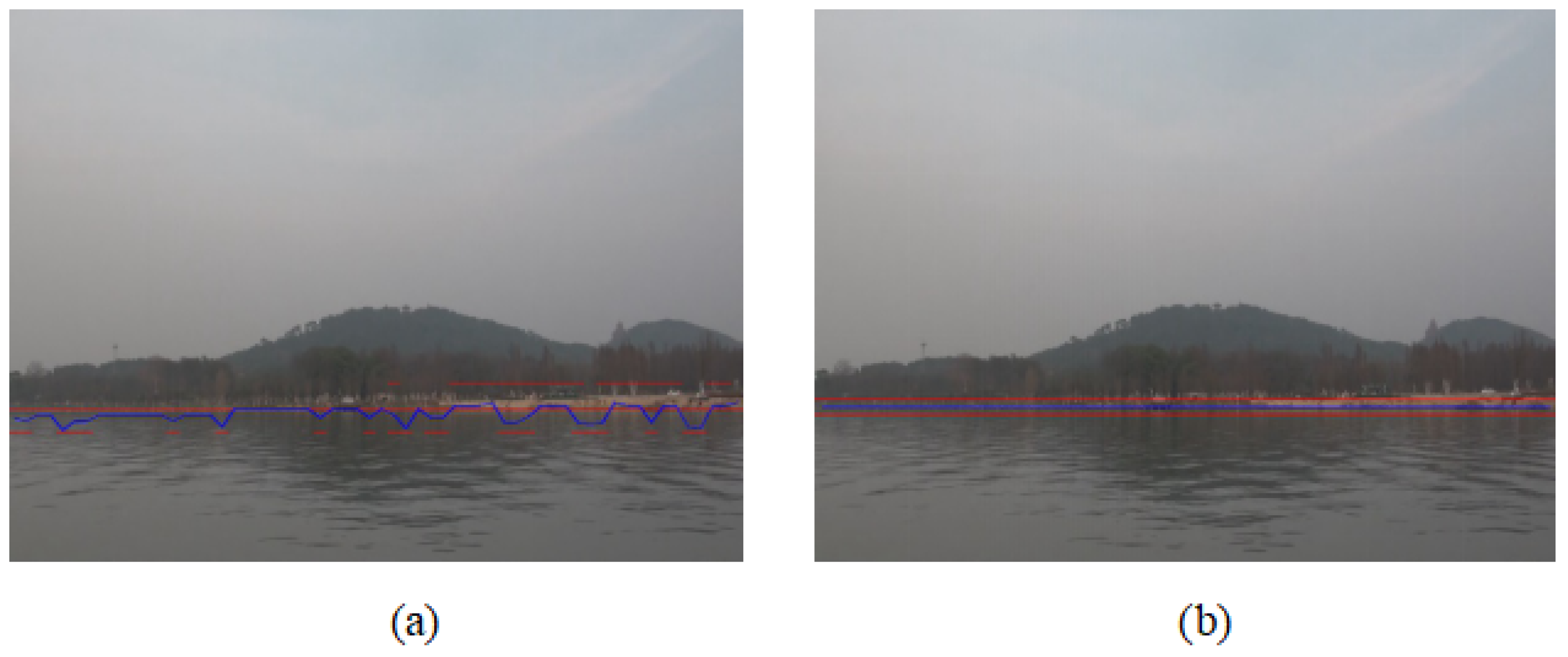
Figure 8 shows the visual results by the Canny edge detector and ours against our concerned environmental noises on waterline detection. In the first row of
Figure 8, all elements in black depict the estimated waterlines by the Canny edge detector. In addition, the second row of
Figure 8 presents our results, in which the blue line indicates the estimated waterlines by our approach.
From
Figure 8, it is observed that our results are obviously better than the compared approach in terms of handling environmental noises. For example, at the top of
Figure 8a–c, rails of our USV, parts of water ripples and shadow are wrongly detected as waterlines, and at the top of
Figure 8d, the real waterlines are not completely detected due to low visibility. In contrast, our estimated waterlines at the bottom of
Figure 8a–d are basically concentrated in the vicinity of ground truth. Therefore, in terms of resisting environmental disturbances, our approach is intuitively superior to the alternative approach.
4.4.2. Quantitative Assessment on Robustness
Then, according to Equations (3)–(6), we have calculated the precision-recall metrics and FP-irrelevance metrics respectively corresponding to the visual results presented in
Figure 8. The quantitative comparisons on these evaluated metrics are shown in
Table 5.
Usually, for a robust waterline detection approach, both high precision and high recall are desired in any water environments. From
Table 5, we see that the edge detection method (Canny edge detector) attains the same desirable recalls as ours when rail, ripple or shadow is emerging, whereas the corresponding precisions are much lesser than ours. Moreover, under foggy weather conditions, despite both of the two compared methods obtain high precision, the recall of the edge detection method is only half of ours. Obviously, for the same scenarios, the effectiveness of the edge detection method is more sensitive to environmental noises than ours. The reason is that a large number of pixels irrelevant to a waterline are also selected by the edge detection method, while correct pixels are annotated in an estimated image-map. For instance, there are 54,182 false positives (FP) also marked as black pixels in the upper image of
Figure 8a. Moreover, although the number of irrelevant pixels is rather small (only 16 false positives) owing to low illumination caused by fog, many true positives are still missing in the result by the edge detection method that induces unsatisfactory recall (just 41.9%). Then, the measured irrelevances shown in
Table 5 indicate that most of irrelevance metrics on the edge detection method are negative, which means those irrelevant pixels (false positives) selected by this method scatter around the real waterline. On the contrary, our irrelevance metrics are positive, implying that our false positives as a whole are more approximate to the ground truth.
Actually, in practical waterline detection tasks, the edge detection method as well as many other alternative approaches such as waterline detection based on image segmentation generally employ necessary image preprocessing (e.g., image denoising) to eliminate those irrelevant pixels induced by environmental noises and guarantee high precision and high recall at the same time. However, these approaches relying on image preprocessing influence the efficiency of waterline detection tasks more or less due to extra computational costs. Instead, our approach can straightforwardly distinguish candidate waterline segments from raw images captured by USVs, since the proposed approach adopts an end-to-end paradigm based on deep learning, in which there is no preprocessing procedure. Therefore, as far as a single estimated image-map is concerned, our approach has better capacity of resisting environmental disturbance in the absence of image preprocessing, which is also demonstrated by the visual comparisons presented in
Figure 8.
4.4.3. Quantitative Assessment on Stability
To evaluate the stability of the waterline detection approach on video data, especially at the moments when environmental factors (e.g., weather or illumination conditions) cause variations in a visual surveillance scenario, we further conduct related experimental comparisons between the edge detection approach and ours. Here, we take foggy conditions bringing about illumination variations as an example, and test their impacts on the stabilities of the two approaches during the procedure that time-sequence images captured by USV are successively dealt with. Correspondingly, we sample 150 image frames from eight hours of video captured by our USV, which cover varied foggy conditions in the same monitoring scenario. Then, based on the precision-recall metrics and FP-irrelevance metrics associated with each of these samples that are achieved, respectively, in terms of Equations (3)–(6), we calculate the stability over the previous four metrics according to Equation (
7), as shown in
Table 6.
In the experiment about stability assessment, to achieve more impartial effect, we practically employ the classic Canny edge detector with necessary image preprocessing as an evaluated edge detection method to compare with ours. From
Table 6, we can see that the measurements of our approach regarding stability over our concerned metrics are closer to zero than the Canny edge detector with image preprocessing, except for the metric FP due to more irrelevant pixels caused by our approach. It indicates that our measuring results over these samples with respect to most of our concerned metrics, e.g.,
precision,
recall and
irrelevance, are more convergent to normal distribution. Therefore, our approach has more stability on the corresponding metrics against environmental variations.
5. Discussion
Visual noises to inland waterlines detection, e.g., linear objects similar to waterline, water ripples, shadow or fog, resulting from the variations of environmental factors usually influence the robustness and stability of the approaches to visually recognize waterlines, thus making it difficult for marine USVs to continually guarantee the effectiveness of vision-based waterline detection approaches in a variable inland water scenario. From the previous experimental results, it can be seen that our deep-learning-based approach achieves much better detection effects compared with traditional approaches. It essentially benefits from an inspiration that deep learning techniques can extract more robust and more discriminative representations (or features) for high-level particular tasks from a large amount of diverse original data by virtue of specific machine learning algorithms, even in the absence of any prior knowledge. Actually, a great deal of current research in computer vision tasks has also confirmed the insight. Motivated with the insight, we proposed a waterline detection approach by devising three specific schemes based on deep learning techniques, i.e., WLpeephole, WLdetectNet and WLgenerateNet, respectively (detailed in
Section 3.1 and
Section 3.2). Among them, WLpeephole is the groundwork of our approach, which accounts for providing WLdetectNet and WLgenerateNet with robust and discriminative waterline features against environmental noises, and further supports their collaboration to effectively accomplish high-level waterline detection tasks. Thus, here, we primarily explain the success of our proposed approach from the perspective of the qualitative visualizations of the deep representations (or features) regarding the WLpeephole-based visually receptive fields under diverse cases.
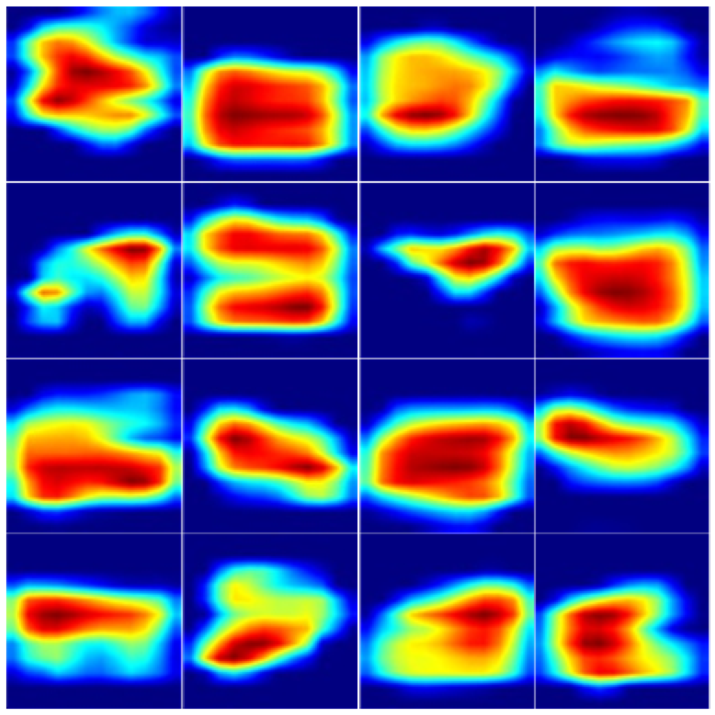
As shown in
Figure 9, we visualize the deep representations of a group of waterline positive samples with certain visual complexity, which are extracted by our deep main network WLdetectNet. From the visualization results in the form of heatmaps, we can see that their highlighted areas just correspond to the areas surrounding waterlines in the WLpeephole-based visually receptive fields (i.e., original image patches), which means human-interpretable concepts related to a waterline have emerged as our deep discriminative features that significantly avail high-level accurate detection tasks about the waterline. This observation coincides with our design principle about WLpeephole (detailed in
Section 3.1), which also verifies our previous assumption about WLpeephole that necessary contextual information in a receptive field can help extract more discriminative representations about the waterline with the aid of a deep neural network. Furthermore, the success of our proposed approach also benefits to some extent from our insight for the scope of WLpeephole since we constrain the WLpeephole as a local receptive field with a certain visual size which can scan across the whole detected image. The advantages of this design are as follows: first, feeding a WLpeephole-based image patch with smaller size to a deep neural network can reduce its computation costs owing to fewer parameters, thus improving the efficiency of our waterline detection; second, arranging the WLpeephole with an appropriate size can compensate for the imprecision of existing edge (or line) detection approaches owing to relying on specific prior knowledge, thus improving the accuracy of our waterline detection.
Although satisfactory results have been achieved in our experiments, there are also some limitations with our approach. For example, there exist some hyper-parameters in our approach, such as the sizes of observing field and recognizing field, whose different values could impact the entire performance of our approach in marine USVs. In addition, the diversity of the training data generated by using WLgenerateNet is critical to improving the robustness of WLdetectNet, whereas the generation of these diverse samples largely depends on the ability of our generative adversarial network.

 ,
, 


