A Manifold-Level Hybrid Deep Learning Approach for Sentiment Classification Using an Autoregressive Model

Abstract

With the recent expansion of social media in the form of social networks, online portals, and microblogs, users have generated a vast number of opinions, reviews, ratings, and feedback. Businesses, governments, and individuals benefit greatly from this information. While this information is intended to be informative, a large portion of it necessitates the use of text mining and sentiment analysis models. It is a matter of concern that reviews on social media lack text context semantics. A model for sentiment classification for customer reviews based on manifold dimensions and manifold modeling is presented to fully exploit the sentiment data provided in reviews and handle the issue of the absence of text context semantics. This paper uses a deep learning framework to model review texts using two dimensions of language texts and ideogrammatic icons and three levels of documents, sentences, and words for a text context semantic analysis review that enhances the precision of the sentiment categorization process. Observations from the experiments show that the proposed model outperforms the current sentiment categorization techniques by more than 8.86%, with an average accuracy rate of 97.30%.

1. Introduction

With easy access to the web, people now interact with brands and products in a whole new way. Whether with physical products or online services, people can share their opinions and reviews immediately on various platforms over the Internet. The world has transformed dramatically as a result of current advancements. Analyzing this large volume of consumer reviews will be helpful for consumers in making an informed decision about a product or service. In social network analyses, the sentiment analysis is an effective method for extracting user thoughts and determining a single user’s sentiments. Social media, with its rich sentiments, has developed into a valuable resource for businesses and governments to understand the opinions and sentiments of online users [1]. For instance, users of Twitter and other social media platforms routinely send out a lot of quick text messages with emoticons to communicate their opinions about various subjects. A textual sentiment analysis (SA) is not just a theoretical approach; it has applications in a variety of fields, including finance [2], education [3], health [4], and other areas.

Machine learning models have drawn a lot of attention recently. Traditional machine learning models almost universally use a two-step procedure. First, some manually created features from the papers are extracted. In a later stage, the features are sent to a classifier that performs predictions. The hand-crafted elements include the bag of words (BoW). Support vector machines (SVM), naive Bayes, gradient boosting trees, random forests, and the hidden Markov model (HMM) are some of the most used classification algorithms. There are various drawbacks to the two-step procedure. To achieve good performance relying on hand-crafted features, this necessitates time-consuming feature engineering and analysis phases. Furthermore, it is challenging to apply the strategy to new positions because it depends on domain expertise for feature creation.

Regarding mobile applications, the majority of apps can freely downloaded and a wide range of possibilities are accessible for a given sort of app, meaning sentiment analyses are made even more challenging. Users usually consult reviews or advice from other users before making decisions. App store owners can use the reviews to increase in the search ranks and catch fraud, while developers can use them to extract feedback (such as features, complaints, and privacy problems) [5]. Manual analyses are quite challenging due to the rapidly increasing volume of reviews (including false and spam reviews). As a result, app reviews have been rated in various ways throughout the last few years, from general exploratory research to categorization, feature extraction, review filtering, and summarizing. Furthermore, evaluations frequently include user opinions, which can be viewed as additional useful meta-data.

To alleviate the restrictions caused by the usage of hand-crafted features, neural techniques have been investigated. These techniques do not require hand-crafted features since they use a machine learning model that converts text into a low-dimensional vector of features. An LSA (latent semantic analysis) was proposed by Dumais et al. [6] in 1989 and was one of the earliest embedding models. An LSA is a trained linear model with 200,000 words and fewer than 1 million parameters. The first neural language model was put forth by Bengio et al. [7] in 2001, and the model worked on a feed-forward neural network that had been trained using 14 million words. The reason they are rarely used is that these early embedding models outperform conventional models with hand-crafted variables. A range of NLP tasks quickly gained popularity for a collection of word2vec models [8] that Google released in 2013, which were trained on 6 billion words. Using Google’s Transformer [9], a fresh NN architecture, in 2018, embedding models were produced by OpenAI. For text-generating projects, their original model, GPT [10], is now extensively used. The same year, Google created BERT [7], a bidirectional Transformer-based system. BERT, which includes 340 million parameters and 3.3 billion words of training data, is currently the most advanced embedding model. It is possible for convolutional neural networks (CNN) [8] to learn local responses from spatial or temporal data, but not sequential correlations. Short-term dependencies in a sequence of data can be handled by recurrent neural networks (RNNs) [9], but long-term relationships are a problem for these networks.

To overcome the constraints of the existing systems in evaluating user sentiments for a certain service or product, a unique methodology based on deep learning utilizing XLNet has been developed. The existing sentiment categorization systems have two issues with handling missing context semantics in text:

i.

The existing studies primarily use language symbol information in texts to classify sentiments. Only a few research have looked at sentiment data with punctuation marks in the dataset. The issue of text context semantics can be resolved with the aid of punctuation symbols that include sentimental information;

ii.

The majority of the ongoing research is focused on the extraction of emotional characterizations and the modeling of textual material at the document level. On the other hand, studies rarely take into consideration doing other levels of text content, such as words or phrases. To overcome the lack of text context semantics in social media assessments, sentiment information can be efficiently collected from many levels via the extraction of sentiment features and by modeling texts from various levels.

Given the above issues in existing models for sentiment classification, a model named the manifold and multi-level sentiment modeling method (MFMLSC) is proposed. Therefore, the main contributions of this work are as follows:

i.

Based on two dimensions, language symbols and emoticon symbols, the manifold sentiment classification method (MFSC) is proposed. In this approach, the problem of text context semantics missing in text reviews is tackled using the word, sentence, and document levels;

ii.

The multi-dimensional sentiment classification method (MDSC) uses two symbol types, i.e., emoticons symbols and linguistic symbols. This approach is used to tackle the problem of missing context information from texts, which plays a significant role in obtaining hidden information from sentiments;

iii.

Based on the effectiveness of these two models, the final model is proposed as the multi-fold and multi-level sentiment modeling method (MFMLSC)

iv.

The proposed model is implemented on three different datasets of Google Pay, Phonpe, and Paytm mobile app reviews. Additionally, the proposed model is validated on the IMDB benchmark dataset.

The rest of the sections are organized as follows. Section 2 discusses the related work. Section 3 provides details and describes the workings of the proposed model. In Section 4, various settings and evaluation parameters are discussed. In Section 5, a summary and the conclusions are presented.

2. Related Work

This section provides a comprehensive review of the recent studies, along with recommended methodologies for addressing sentiment analysis challenges based on word embedding and deep learning (DL) techniques. Next, the state-of-the-art literature is addressed, with a focus on sentiment analyses in different areas.

Over the last two decades, the classification of user sentiments has attracted an increasing number of scholars and yielded a large number of research findings [10]. The classical machine learning and deep learning methods for classifying emotions mostly depend on supervised learning. The challenge is that natural language processing relies on efficient word embedding. By thoroughly training the global word–word co-occurrence of statistical data from the corpus, Mikolov et al. [11] and Pennington [12] first revealed that word vectors are learned through an RNN. As seen in [13], the final global vector (GloVe) has an intriguing linear substructure in the word vector space. Tang et al. [14] offered three models that took into account the text’s emotional propensity and learned word embeddings with the sentiment. Word2Vec embedding was used in [15] to perform a sentiment analysis on reviews received from the Indonesian website Traveloka. It is estimated that their model is 91.9% accurate. The authors of [16] presented a monitoring system based on DL and ontology to aid the traveling process. Fuzzy ontologies and Word2vec embeddings were utilized to construct the suggested system’s feature extraction module; the BiLSTM model was then used to classify the input text. According to Facebook, TripAdvisor, and Twitter data, the proposed technique was tested and found to be 84% accurate in its predictions.

A multi-layer architecture for customer evaluation approaches (such as word embedding and compositional vector models) was proposed in [17]. A back-propagation technique was used to train the network and provide weights for the various aspects of the design once it had been integrated into a neural network. GloVe-DCNN, a brand-new device featuring a variety of sentimental qualities, was introduced in [18]. Word embedding, n-grams, and the polarity score properties of sentiment words were used to create a deep CNN. The authors of [19,20,21] developed a document representation system using the fuzzy bag of words paradigm (FBoW). An enhanced FBoW model that replaces the initial hard planning module with the Word2vec approach using fuzzy mapping was developed by replacing the original module with the Word2vec embedding. To determine the degree of similarity between words and clusters in seven different real-world document datasets, the researchers used three different approaches.

For the identification and condition analysis of traffic accidents, the authors of another study proposed a system based on using ontology with LDA (OLDA) and a BiLSTM network [22]. OLDA was employed in the proposed system to extract data and label texts. As a result, classifiers such as FastText and BiLSTM are employed. This system was more accurate than the previous one. In another study, BiLSTMs were used to gather data on the long-term reliance on word and sentence locations [23]. A CNN and BiLSTM were combined in the suggested hybrid strategy. LSTM outputs from sentence classification are applied to the multi-channel CNN to produce n-gram features. To find ADRs (adverse drug reactions) in electronic medical data, the authors of [24] suggested using a deep learning approach (EHRs). The proposed approach used the joint AB-LSTM model and embeddings based on lemmas to locate ADRs. The proposed technique had an F-measure of 73.3% on the EHR dataset. The combined model, for example, outperformed previous models that used a stack of CNNs and LSTM deep learning models, as shown in [25]. The dataset representation of Word2Vec is preferable to Word2Seq. Sentiment-based and dictionary-based representations of texts are some of the ways that texts are encoded. For extracting sentence features, the CNN model is paired with three attention methods. They concluded that the proposed CNN models were the most effective of all the models considered.

According to Hameed and Garcia-Zapirain [26], the accuracy of the BiLSTM approach was 85.8% on the IMDB Movie Review and SST2 (Stanford Sentiment Treebank) datasets [27]. The authors demonstrated that the BiLSTM method is both more efficient and suitable for sentiment analysis problems. Word2Vec, LSTM, RNN, and CNN methods were utilized by Xu and colleagues [28] to extract emotions from Chinese hotel reviews. The model with the highest F-score, 92%, was the BiLSTM method.

Some researchers have proposed hybrid deep learning-based models to improve accuracy, such as the LSTM-CNN grid-search (GS) approach for Amazon and IMDB reviews [29]. The authors utilized a grid-search technique and compared it to CNN, LSTM, CNN–LSTM, and other approaches. Their model outperformed several baseline models with an overall accuracy of 96%. In a similar study, the researchers [30] used Amazon reviews to model topics before using a CNN to identify views. The authors stated that their proposed approach improved the accuracy by 6 to 20% in comparison with the established methods.

Further studies were conducted on the more efficient embedding approach, BERT, and its derivatives in enhancing the analysis of sentiments for user reviews. The authors of [31] employed BERTCNN to improve a sentiment analysis for commodities reviews, with the results stating that the BERT-CNN (F1-score of 84.3%) outperforms the BERT (82%) and CNN (84.3%) (70.9%) approaches. Similarly, in [32] the SenBERT-CNN (sentiment BERT-CNN) was proposed for analyzing the feedback for JD.com, a mobile phone supplier, by merging the BERT and CNN approaches to obtain deep characteristics of the dataset. When the LSTM, BERT, and CNN approaches were compared, the authors found that BERT-CNN worked the best, with a score or 95.7%. In [33], on the other hand, a dataset from Drugs.com was used to develop neural network models for predicting reviews of drugs. On a scale from 0 to 9, patients’ levels of happiness were given scores between 0 and 9. The authors tested many neural network models, including the BERT-LSTM model, with the following methods: 10-class and 3-class compressed forms of the dataset. The results showed that the BERT-LSTM model was the best-suited for the 3-class setup, even though it took a very long time to train. Others examples include [34], who used BERT to train different NN models on a dataset of movie reviews. The results showed that BERT was the most accurate, while [35] used BERT to analyze Twitter sentiments by turning jargon into plain text for BERT training.

Additionally, in [36], the authors suggested a deep learning model using BERT for ADE (adverse drug effect) retrieval and detection to find pharmacological side effects. As a classifier and retrieval tool, the proposed model utilized sentence structure feature embeddings and BERT. Furthermore, in [37], the authors developed a method for extracting medical relations that relied on a pre-trained technique and a mechanism of fine-tuning rather than manual labeling. For feature extraction, the suggested method combined the BERT architecture with one-dimensional convolutional neural networks (1D-CNNs). The suggested method was tested on three datasets: the BioCreative V chemical relation corpus of illness, a classical Chinese literature dataset, and the i2b2 2012 temporal relation challenge dataset, and F1 score values of 0.7156, 0.8982, and 0.7085, respectively, were obtained. It was proposed by Ma et al. [38] that an enhanced version of Sentic LSTM be used for a joint task that combined the target-dependent detection of aspects and targeted aspect-based polarity classification. In another study, Sentic LSTM was developed by Ma et al. for the explicit integration of explicit and implicit information. By refining pre-trained word vectors with scores of sentiment intensity provided by sentiment lexicons, Gu et al. [39] presented a word vector refinement method that improved each word vector and performed better in the sentiment analysis. Hashida et al. [40] created a hybrid paradigm of multi-channel decentralized representation for textual data.

Various pre-trained language models, such as ELMo [41], BERT [42], and GPT [43], have recently demonstrated effective performance. Various Transformer-based language models such as BERT [42], robustly optimized BERT pre-training approach (RoBERTa) [44], and a lite BERT for self-supervised learning language representations (ALBERT) [45], have recently obtained the highest performance in many NLP tasks. Transformer’s bidirectional encoder representation is known as BERT. Position embedding and word embedding are included in BERT’s inputs. BERT’s feature representation layers, unlike those of 1D-CNN and LSTM, rely on both left and right context information. A more advanced embedding technique, known as BERT, was also found to be useful in improving the sentiment analysis of reviews. Another study [46] examined the sentiment analysis performance of the SVM, multi-nomial naive Bayes, LSTM, and BERT approaches. Stemming, tokenization, lemmatization, and punctuation removal were among the preprocessing techniques used. The dataset includes 1.6 million tweets classified as good or negative. The study determined that BERT’s performance was the best, with an accuracy rate of 85.4%. Two deep learning algorithms were created by the authors of [47] for the analysis of sentiments in multi-lingual social media text. During Pakistan’s 2018 general election, Twitter was used to gather data. 80% of the dataset was used for training and 20% for testing. The XLM-RoBERTa and multi-lingual BERT (mBERT) from Transformer approaches were studied for their performance in this regard (XLM-R). The mBERT learning rate was set to 2 × 10⁻⁵, and the XLM-R learning rate was set to 2 × 10⁻⁶ during the hyperparameter tweaking. Furthermore, mBERT had a precision rate of 69%, while XLM-R had a precision rate of 71%, according to the results of the trial. Using a deep bidirectional long short-term memory (DBLSTM) approach, in [48] the sentiments of Tamil tweets were analyzed. The dataset contains 1500 tweets categorized as either positive, negative, or neutral. The data were cleaned and pre-trained using the Word2Vec model before being represented using the DBLSTM word embedding approach. Furthermore, 80% of the dataset was utilized for training and 20% for testing. The DBLSTM approach was shown to be 86.2% accurate in the research. In a recent study [49], the authors proposed an adversarial strategy for handling the domain shift problem. The adversarial meaning stems from the parallel structure designed between the loss function on training samples and that on test samples. Using a projector and classifier, they presented a theoretical analysis of several benchmark datasets. In [50], the researchers performed a survey on an aspect-based sentiment analysis (ASBA). The authors showed a comparison of several techniques used in the ASBA.

In recent years, numerous studies have presented deep-learning-based sentiment assessments, each with its own set of characteristics and performance results. The traditional method for sentiment analyses is suitable for dealing with the categorization of small-scale texts. In the face of huge amounts of data, the analytical efficiency is low, and locating sentiment information is challenging. In recent years, deep learning approaches have demonstrated promising accuracy and efficiency in textual data sentiment classification. With the advent of Transformer-based pre-trained representations, the accuracy and efficacy have increased dramatically. Consequently, this study investigates and proposes a unique sentiment classification model based on the deep learning technique and XLNet’s autoregressive pre-trained model.

3. Proposed Model

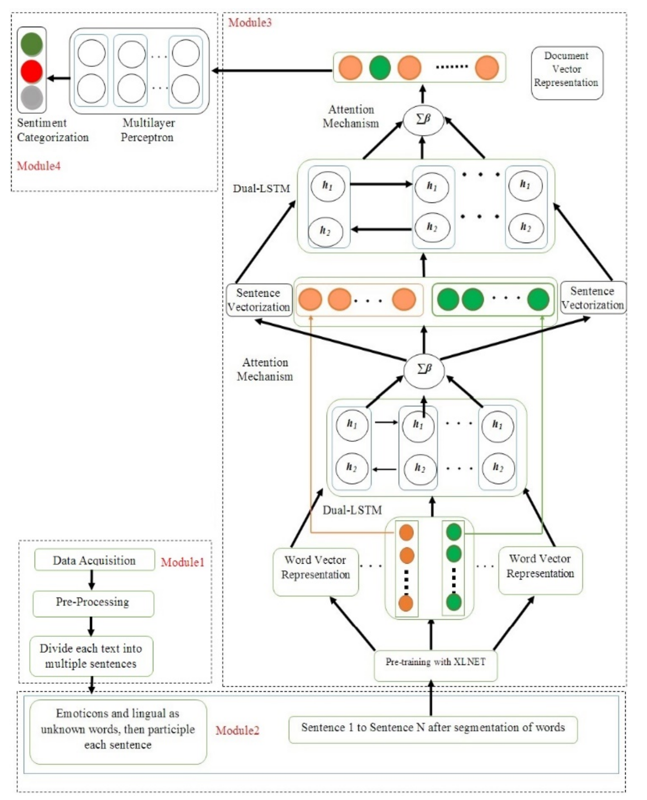
The proposed model primarily consists of two major components. Manifold emotion modeling is a technique that incorporates three different components: words, sentences, and documents. The second method makes use of language and punctuation marks to model multi-dimensional sentiments in two dimensions. Each word in the dataset is broken up into its unique phrase by using emoticons as separators. Through the practice of regarding emoticons and linguistic markings as unrecognized words, every sentence is segmented utilizing the word segmentation methodology that is currently in use. A technique for modeling the emotions associated with textual material is presented with three levels: word, phrase, and document. A multi-dimensional technique for classifying sentiment is given for modeling the text content using two dimensions: language-based symbols and emoji symbols at the word and sentence level.

The multi-fold with multi-level modeling results are inputs into the multi-level perception network using the pre-trained autoregressive word representation model XLNet to produce the final sentiment classification results (Figure 1). The algorithm of the proposed model is shown as Algorithm 1.

Algorithm 1: Multi-Fold Dimensional Modeling Method for Sentiment Classification

1: input: IDocument 2: output: IDocumentDVector 3: initialization of the XLNet and Dual-LSTM models 4: IDocumentSVector = [] 5: for each sentence in IDocument: 6: for each W_word, emoji in sentence: 7: WVector = BERT(W_word) 8: L_languageWVector = XLNet (L_language) 9: P_emoticonsWVector = XLNet (P_emoticons) 10: sentence WVector = [WVector, emoticon WVector] 11: SVector = Attention(Dual-LSTM(S WVector)) 12: L_languageSVector = L_languageWVector 13: sentence SVector = [SVector, L_languageSVector] 14: IDocumentSVector += sentence SVector 15: IDocumentDVector = Attention(Dual-LSTM(IDocumentSVector))

The proposed model is divided into four modules. The module-wise discussions of the proposed model are presented below.

3.1. Pre-Processing

The goal of the pre-processing phase is to remove all extraneous words from the corpus.

The following are the major stages of the pre-processing phase:

i.

Using the WordPiece tokenization paradigm, each word in the social input text is tokenized and can be broken into several sub-words;

ii.

The Natural Language Toolkit (NLTK) removes stop words (is, the, a, etc.);

iii.

Slang is converted to more formal forms;

iv.

By eliminating texts that include indentations or by employing a widely unused set of suffixes and indentations, such as “-ing” or “pre-,” one can restore extracted words to the word stem format using a rule-based stemmer technique;

v.

Lemmatization removes inflection endings and returns words to the dictionary format. The proposed approach utilizes the NLTK suffix-dropping algorithm for stemming and lemmatization to improve the lexical context and analysis;

vi.

Uppercase characters are converted to lowercase characters and repeated characters to their generic form;

vii.

Spelling corrections are made using the Levenshtein distance and by selecting misspelled keywords.

Punctuation marks are used to divide cleaned and pre-processed texts into sentences. Punctuation is a collection of symbols that control and clarify the contents of various texts. Punctuation serves to clarify the meanings of texts by connecting or separating words, phrases, and clauses. As a result, punctuation is used to transform words into sentences.

XLNet

XLNet is a novel NLP pretraining approach that produces cutting-edge outcomes on several NLP tasks. Autoregressive (AR) language modeling and autoencoding (AE) are two pretraining aims for pretraining neural networks used in transfer learning NLP that have been proven effective. While avoiding the limitations of the two types of language pretraining objectives (AR and AE), XLNet incorporates concepts from both.

3.2. Multi-Fold Sentiment Modeling Method (MFSC)

The majority of the current research focuses on document-level text content modeling and sentiment feature extraction, with minimal attention paid to the interaction and correlation among sentences in the document. Between successive sentences in the text, there are evident progressive (forward) and adversative (reverse) linkages, as well as clear correlation and reciprocal influences between terms. As a result, the technique is suggested here for multi-fold sentiment modeling. The extraction of sentiment features and modeling content of text at several levels, such as words, phrases, and documents, helps address the lack of context semantics in dataset texts.

The multi-fold sentiment modeling method has three stages, the (i) word, (ii) sentence, and (iii) document levels. In the first fold of words, the input is the outcome of the segmentation `of sentences. The outcome of this process is the representation of the word vector for the given sentences. In the second fold, i.e., the sentence level, the input for the model is the representation of vectorized words of the given set of sentences, and the outcome is the representation of vectorized sentences from the set of sentences. The multi-dimensional sentiment model is described in detail in the next section. The vectorized collection of several sentences is provided as the input in the document fold, and the result is the vectorized document.

The specifics at the document level are listed below.

i.

Based on the grammatical rules and conjunctions between sentences, two types of relations are obtained: forward relations and reverse relations;

ii.

The attention-based network is provided with prior knowledge of the following two types of relationships between sentences. Sentences with a reverse connection should have opposing sentiment polarities as much as is feasible. Sentences with forwarding relationships should have uniform sentiment polarity as much as is feasible. An attention-based system at the sentence level that is based on relationship constraints between sentences is provided here. This mechanism takes into account the two different sorts of linkages that exist between sentences. In the research, the attention-based method utilizes the attention formula at the phrase level;

iii.

The vectorized text of every phrase is provided as the input for the dual-LSTM network based on the limitations of the attention-based mechanism, and the vectorized view of the given document is collected.

An output for sentiment categorization is generated by a multi-layer perception network using the representation of a vectorized document that has been obtained. Equation (1) provides a definition of the sentiment classification function that is based on multi-fold and multi-dimensional sentiment modeling:

$$\underset{x}{\min }{{\displaystyle \sum }}_{j=1}^M{\left(x^T{y}_j-z_j\right)}^2+{\partial }_1{x}_1+{\partial }_2{{\displaystyle \sum }}_{j=1}^M{{\displaystyle \sum }}_{k\ne j}{S}_{jk}{\left({\omega }_j-{\omega }_k\right)}^2+{\partial }_3{{\displaystyle \sum }}_{j=1}^M{{\displaystyle \sum }}_{k\ne j}{P}_{jk}{\left({\mu }_j-{\mu }_k\right)}^2$$

(1)

Here, the total number of texts is represented by M, which represents the model of the sentiment classification; $y_j$ is the representation of the vector of the jth text $\mathrm{and} z_j$ is the sentimental orientation of the jth text; ${\omega }_j$ and ${\omega }_k$ is the factor of attention for the word level; ${\mu }_j \mathrm{and} {\mu }_k$ is the factor of attention for the sentence level; $S_{jk}$ is the factor of similarity of sentiment text j and sentiment phrase k; $P_{jk}$ is the similarity factor of sentence j and sentence k; ${\partial }_1$, ${\partial }_2$, and ∂₃ represent the various hyperparameters.

3.3. Multi-Dimensional Sentiment Classification Method (MDSC)

The primary actions involved in multi-dimensional sentiment modeling at the level of individual words are discussed below:

(1)

Since emoji and linguistic data provide information about sentiments, the dataset that contains emoji and linguistic symbols is used as the input to the language model, i.e., pre-training XLNet;

(2)

Emojis and linguistic symbols are processed in the same way as sentiment words when a pre-trained model is used to model information available on social networks. This leads to the creation of the linguistic symbol word vector as well as the emoticons symbol word vector. This combination produces a multi-dimensional representation of the text’s emotions.

The following are the primary steps in the multi-dimensional sentiment modeling at the sentence level:

i.

The attention network provides prior knowledge of sentimental words. An approach based on word-level attention on the dictionary of sentiment restriction is provided, with the attention coefficients of sentiment-related words being as similar as possible. The attention formula is based on the attention formula at the word level;

ii.

Vectorized words of language symbols and emoji symbols are given as inputs to a dual-LSTM network integrated with attention; the output is received as the vector of sentences of language symbols;

iii.

The vectorized words of the emoji symbols are taken as outputs as the vectors of sentences of the emoji symbols directly;

iv.

Combining the obtained sentence vectors of language symbols with emoticon symbols yields the sentence vectors.

The detailed mechanism of sub-modules is discussed below.

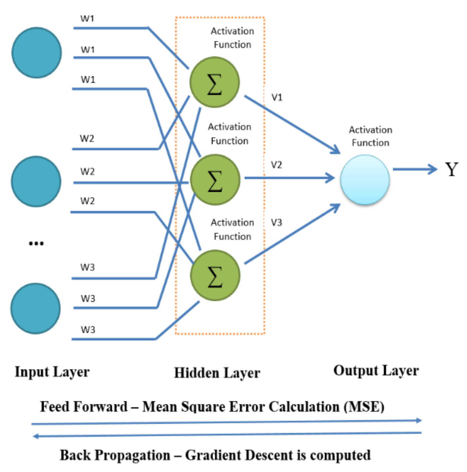
3.4. Sentiment Classification Using Multi-Layer Perceptron

The document vector representation is fed into a multi-level perceptron. The following parameter settings shown in

Table 1. Parameter settings for the MLP.

Parameters	Values
Optimization function	sgd (Stochastic Gradient Descent)
Batch-Size	64
Learning rate	0.03
Number of iterations	20
Activation Function	ReLu
Epochs	50

are used in obtaining optimized performance during sentiment classification. These parameters are obtained by performing several experiments with different parameters.

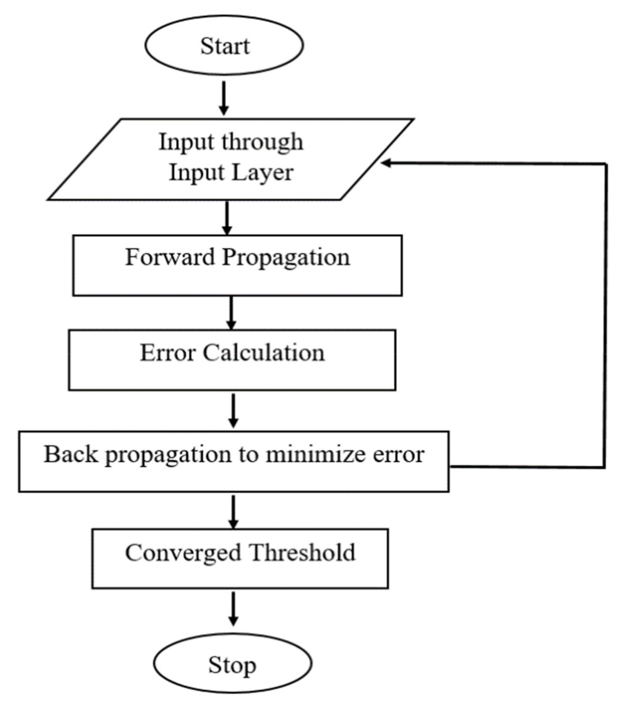
Using the above parameters in Table 1, the multi-layer perceptron (as shown in Figure 2) goes through the learning process and the output class labels are obtained using the below process, the MLP learning Procedure, as shown in Figure 3.

i.

Using forward propagation, the data from the input layers are transmitted to the output layer;

ii.

The error is calculated based on the received output (the difference between the predicted outcome and the achieved outcome);

iii.

The error is back-propagated and its derivatives are obtained concerning all weights in the network, then the model is updated.

These three steps are repeated over multiple epochs to learn the ideal weights. Finally, the output is achieved through a threshold function to obtain the predicted class labels.

The error, i.e., the mean square error, is calculated using the following equation:

$${\Delta }_w\left(t\right)=-\in \frac{dE}{d{w}_{\left(t\right)}}+\propto {\Delta }_w\left(t-1\right)$$

(2)

Here, ${\Delta }_w\left(t\right)$ is the gradient of the current iteration, $\in$ is the bias, $dE$ is the error in each iteration, the weight vector is represented by $d{w}_{\left(t\right)}$, $\propto$ represents the learning rate, and the gradient of the previous iteration is denoted by ${\Delta }_w\left(t-1\right).$

This process continues until each input–output pair’s gradient has converged, which means the freshly computed gradient has not changed more than the set convergence threshold since the previous iteration. Here, the network updates are performed incrementally.

4. Results and Discussion

4.1. Data Acquisition

Using the Google Play Scraper package with Python APIs, the dataset for three popular UPI mobile payment apps were collected. The three payment apps were GooglePay, PhonePe, and Paytm. Google Play Scraper offers Python APIs for crawling the Google Play Store without external dependencies. The details of the dataset obtained are as shown in

Table 2. Datasets.

Dataset	Total Reviews	Positive	Negative
GooglePay	45,597	20,975	24,622
PhonePe	43,209	17,715	25,494
PayTM	47,932	33,073	14,859

. Here, we considered only positive and negative reviews, while neutral reviews were not considered.

In this process, the equations are numbered consecutively, with equation numbers shown in parentheses flush with the right margin of the column, as in (1). First, use the equation editor to create the equation. Then, select the “Equation” markup style. Press the tab key and write the equation number in parentheses. To make your equations more compact, you may use the solidus (/),exp function, or appropriate exponents. Use parentheses to avoid ambiguities in denominators. Punctuate equations when they are part of a sentence, as in:

B_p + H₂ = 40.

(3)

4.2. Data Augmentation

A balanced dataset facilitates the establishment of unambiguous decision limits for every class and enables models for the classification of data more precisely in any classification task. Any unbalanced dataset can be converted to a balanced one using data augmentation techniques, guaranteeing that the dataset is consistent across labels. The algorithm is named SMOTE [51], and is a commonly used data augmentation approach that may be used for any dataset without any influence on predictions based on a particular label. SMOTE samples the class with a minority with the help of a k-nearest neighbours classifier; it selects samples close to the feature space and generates synthesized data points. In this study, we use SMOTE to balance the dataset in terms of the labels and performs an evaluation.

4.3. Performance Measurement

To assess how well the suggested model works, an accuracy matrix is computed. For positive sentiment classification, true positive and false positive variables are identified. For negative sentiment classification, the true negative and true positive variables are defined as shown in

Table 3. The accuracy parameters.

	Positive Class	Negative Class
Identification of Positive Class	X1 = True Positive	Y1 = False Positive
Identification of negative Class	X2 = False Negative	Y2 = True Negative

.

Using the parameters in Table 3, the following equation is defined to assess the accuracy of the proposed model:

$$\mathrm{Accuracy}\left(\mathrm{Z}\right)=\frac{X_1+X_2}{Y_1+Y_2+X_1+X_2}$$

(4)

4.4. Performance Evaluation

For a clear view of and simplicity in the graphical representations, the models are termed hereafter as shown in

Table 4. The models and their aliases.

Models	Alias
CNN with Word2Vec	MO-01
BiLSTM with Word2Vec	MO-02
CNN with BERT	MO-03
BILSTM with BERT	MO-04
MFSC with CNN and Word2Vec	MO-05
MFSCwith CNN and BERT	MO-06
MFSC with BiLSTM and Word2Vec	MO-07
MFSCwith BiLSTM and BERT	MO-08
MFSCwith XLNet	MO-09

.

A hyperparameter is a value for a parameter that is used to influence the learning process. Different hyperparameters are tuned for optimized performance accuracy. Comprehensive experiments are performed using several hyperparameters, such as the embedding type, activation function, and dropout.

The deep learning methods CNN and BiLSTM with different word embedding methods, i.e., Word2Vec and BERT, are tested on different hyperparameters. The proposed model is also tuned with several hyperparameters. The hyperparameter tuning process is performed with different embedding combinations on 200, 300, and 400 words and with learning rates ranging from 0.01 to 0.10. The observations of these experiments are shown in

Table 5. The performance accuracy (%) for an embedding size of 200.

Dropout = 0.01				Dropout = 0.02				Dropout = 0.03
Models	Dataset 1	Dataset 2	Dataset 3	Models	Dataset 1	Dataset 2	Dataset 3	Models	Dataset 1	Dataset 2	Dataset 3
M01	61.66	60.35	62.33	M01	65.36	61.33	64.12	M01	66.19	64.32	62.15
M02	66.36	65.21	66.33	M02	61.32	64.22	62.14	M02	63.20	62.55	61.32
M03	70.66	68.55	68.32	M03	68.55	69.56	68.22	M03	64.32	66.25	65.32
M04	72.33	74.25	70.25	M04	71.42	72.22	70.65	M04	70.62	69.32	71.25
M05	81.65	81.56	83.22	M05	80.62	82.65	81.24	M05	81.55	84.12	83.85
M06	84.11	80.35	81.25	M06	82.15	81.25	83.36	M06	88.85	83.54	84.98
M07	86.32	84.25	83.22	M07	87.65	84.26	84.11	M07	91.65	89.55	89.99
M08	88.35	87.15	85.25	M08	89.22	88.95	88.01	M08	85.95	86.32	84.62
M09	93.28	91.56	92.36	M09	92.69	90.33	91.56	M09	95.62	95.05	95.99
(a)				(b)				(c)
Dropout = 0.04				Dropout = 0.05				Dropout = 0.06
Models	Dataset 1	Dataset 2	Dataset 3	Models	Dataset 1	Dataset 2	Dataset 3	Models	Dataset 1	Dataset 2	Dataset 3
M01	70.15	69.66	70.69	M01	68.35	64.69	66.35	M01	64.20	60.17	62.96
M02	72.66	73.21	73.65	M02	69.36	68.32	67.35	M02	61.32	62.65	60.98
M03	71.15	75.11	76.02	M03	61.25	62.35	61.22	M03	65.21	67.32	67.06
M04	77.62	78.65	77.12	M04	69.36	70.32	68.33	M04	70.26	71.06	69.49
M05	82.15	83.62	84.12	M05	84.63	83.98	84.05	M05	85.77	84.12	83.85
M06	86.66	85.95	86.01	M06	82.65	81.63	80.62	M06	85.19	83.54	84.98
M07	90.65	90.36	91.65	M07	91.65	90.61	89.63	M07	91.20	89.55	89.99
M08	92.15	91.62	92.99	M08	86.63	87.65	89.65	M08	87.97	86.32	84.62
M09	96.33	95.95	96.36	M09	94.32	95.62	93.64	M09	95.22	95.05	95.99
(d)				(e)				(f)
Dropout = 0.07				Dropout = 0.08				Dropout = 0.09
Models	Dataset 1	Dataset 2	Dataset 3	Models	Dataset 1	Dataset 2	Dataset 3	Models	Dataset 1	Dataset 2	Dataset 3
M01	65.32	64.12	63.25	M01	66.30	62.27	65.06	M01	62.10	63.43	61.76
M02	64.15	64.32	66.21	M02	68.74	67.70	66.73	M02	66.41	66.58	68.47
M03	61.15	62.35	65.32	M03	72.00	75.96	76.87	M03	60.60	61.70	60.57
M04	72.55	71.65	72.36	M04	69.07	69.87	68.30	M04	75.80	81.65	75.61
M05	83.15	84.13	85.65	M05	84.10	85.08	86.60	M05	85.08	86.06	87.58
M06	80.75	81.73	83.25	M06	88.31	87.60	87.66	M06	83.81	82.79	81.78
M07	85.82	86.80	88.32	M07	88.59	85.20	85.05	M07	93.91	92.87	91.89
M08	82.75	86.32	85.25	M08	90.16	89.89	88.95	M08	89.98	91.00	93.00
M09	90.72	91.70	93.22	M09	93.63	91.27	92.50	M09	93.97	92.65	93.29
(g)				(h)				(i)
				Dropout = 0.10
				Models	Dataset 1	Dataset 2	Dataset 3
				M01	65.95	84.32	63.88
				M02	69.93	68.89	67.92
				M03	67.41	88.65	69.26
				M04	83.89	84.87	86.39
				M05	79.83	81.30	81.80
				M06	87.47	88.45	89.97
				M07	87.57	88.59	90.59
				M08	91.63	90.35	93.32
				M09	96.62	94.32	95.32
				(j)

and

Table 6. The performance accuracy (%) for an embedding size of 300.

Dropout = 0.01				Dropout = 0.02				Dropout = 0.03
Models	Dataset 1	Dataset 2	Dataset 3	Models	Dataset 1	Dataset 2	Dataset 3	Models	Dataset 1	Dataset 2	Dataset 3
M01	67.36	64.32	68.62	M01	71.22	70.39	70.84	M01	72.32	72.32	72.32
M02	70.35	72.15	72.44	M02	72.51	72.87	72.42	M02	66.36	65.32	67.33
M03	74.22	73.12	71.56	M03	74.84	75.48	75.88	M03	61.63	62.36	64.36
M04	63.00	83.65	82.22	M04	76.48	77.51	75.98	M04	74.33	73.66	72.35
M05	95.65	91.59	94.22	M05	91.12	90.65	93.32	M05	84.36	83.22	86.35
M06	86.31	84.32	87.35	M06	89.25	88.65	85.65	M06	88.25	87.56	86.32
M07	92.56	93.32	91.21	M07	90.32	92.35	90.36	M07	90.65	91.63	91.54
M08	84.56	85.12	85.58	M08	93.65	94.62	92.65	M08	89.99	87.25	88.63
M09	92.36	94.25	91.35	M09	94.56	95.65	93.65	M09	96.32	94.32	95.33
(a)				(b)				(c)
Dropout = 0.04				Dropout = 0.05				Dropout = 0.06
Models	Dataset 1	Dataset 2	Dataset 3	Models	Dataset 1	Dataset 2	Dataset 3	Models	Dataset 1	Dataset 2	Dataset 3
M01	72.36	71.53	71.98	M01	70.51	67.47	71.77	M01	69.35	67.32	68.35
M02	73.65	74.01	73.56	M02	73.50	75.30	75.59	M02	72.12	71.15	73.65
M03	75.98	76.62	77.02	M03	77.37	76.27	74.71	M03	75.65	74.36	76.32
M04	77.62	78.65	77.12	M04	81.32	84.36	83.32	M04	84.35	81.36	82.35
M05	84.92	85.63	86.01	M05	85.21	86.07	84.14	M05	86.32	87.18	85.25
M06	87.16	87.9	88.1	M06	83.21	84.21	85.00	M06	84.32	85.32	86.11
M07	91.21	91.56	92.01	M07	89.14	90.41	88.25	M07	90.25	91.52	89.36
M08	93.63	94.01	93.9	M08	87.42	86.04	85.21	M08	88.53	87.15	86.32
M09	97.23	97.65	97.01	M09	95.14	93.21	94.77	M09	96.25	94.32	95.88
(d)				(e)				(f)
Dropout = 0.07				Dropout = 0.08				Dropout = 0.09
Models	Dataset 1	Dataset 2	Dataset 3	Models	Dataset 1	Dataset 2	Dataset 3	Models	Dataset 1	Dataset 2	Dataset 3
M01	73.83	70.79	75.09	M01	72.16	71.33	71.78	M01	72.90	71.93	74.43
M02	74.84	75.20	74.75	M02	72.88	74.68	74.97	M02	77.10	77.46	77.01
M03	76.16	75.06	73.50	M03	76.83	77.47	77.87	M03	76.72	75.62	74.06
M04	80.07	83.11	82.07	M04	83.16	80.17	81.16	M04	83.32	81.65	85.32
M05	86.37	87.23	85.30	M05	87.32	88.18	86.25	M05	86.33	84.12	85.22
M06	84.37	85.37	86.16	M06	88.81	89.55	89.75	M06	84.21	86.32	82.55
M07	90.30	91.57	89.41	M07	91.26	93.29	91.30	M07	91.56	90.21	91.24
M08	88.58	87.20	86.37	M08	94.59	95.56	93.59	M08	92.56	91.25	91.11
M09	96.30	94.37	95.93	M09	95.50	96.59	94.59	M09	95.62	94.12	95.22
(g)				(h)				(i)
				Dropout = 0.10
				Models	Dataset 1	Dataset 2	Dataset 3
				M01	74.46	84.32	75.72
				M02	74.07	75.87	76.16
				M03	77.85	88.65	78.52
				M04	85.14	82.93	84.03
				M05	87.53	88.39	86.46
				M06	85.53	86.53	87.32
				M07	91.46	92.73	90.57
				M08	89.74	88.36	87.53
				M09	97.46	95.53	97.09
				(j)

.

The above Table 5 provides the performance accuracy rates of different models with an embedding size of 200 with dropout from 0.01 to 0.10. All models M01, M02, M03, M04, M05, M06, M07, M08, and M09 are tested using this combination. It can be observed that the proposed model achieves the highest classification accuracy rate of 96.62% using a dropout rate of 0.10 for dataset 1.

For dataset 2, the highest accuracy can be observed for the dropout of 0.04 with 95.95% accuracy. At the same time, 96.36% accuracy is obtained for dataset 3 at a dropout rate of 0.04. The accuracy rates of the other models vary depending on the different dropout values. Overall, the proposed model shows the highest performance in terms of classification accuracy as compared to the other eight models.

Table 6 shows the classification accuracy performance for the embedding size of 300 and with dropout rates ranging from 0.01 to 0.10. As per the observations for the above figure, it is clear that none of the models shows consistent performance. For example, model M01 shows an accuracy rate of 67.36% for dataset 1, but for dataset 2 the accuracy decreases to 64.32%, and again the model achieves a higher accuracy rate of 68.62% for dataset 3, with a dropout rate of 0.01. Model M02 achieves its highest accuracy rate of 77.46% for dataset 2 with a dropout rate of 0.09, whereas the lowest accuracy rate of 67.33% is achieved with a dropout rate of 0.04. The observations from the experiments with an embedding size of 300 and dropout rate of 0.03 indicate that this combination with other hyperparameters has shown consistent performance for all models.

Table 7. The performance accuracy (%) for an embedding size of 400.

Dropout = 0.01				Dropout = 0.02				Dropout = 0.03
Models	Dataset 1	Dataset 2	Dataset 3	Models	Dataset 1	Dataset 2	Dataset 3	Models	Dataset 1	Dataset 2	Dataset 3
M01	64.32	66.33	65.24	M01	66.55	67.36	68.22	M01	62.35	66.35	64.21
M02	66.55	64.32	62.33	M02	68.36	67.21	69.36	M02	66.32	67.24	65.32
M03	68.36	68.32	70.56	M03	70.22	71.56	72.32	M03	70.25	69.68	71.56
M04	70.25	71.52	72.22	M04	72.36	73.32	71.35	M04	74.65	73.22	74.01
M05	74.36	76.32	72.52	M05	75.62	78.32	74.22	M05	76.32	77.25	74.35
M06	76.32	78.25	77.85	M06	77.55	75.22	76.32	M06	81.65	82.54	80.26
M07	84.66	85.65	83.26	M07	79.65	80.25	91.56	M07	84.68	85.10	86.32
M08	89.56	88.32	90.23	M08	84.32	82.35	83.77	M08	89.62	90.21	91.25
M09	94.35	94.56	93.26	M09	90.21	91.36	91.55	M09	94.56	95.21	94.96
(a)				(b)				(c)
Dropout = 0.04				Dropout = 0.05				Dropout = 0.06
Models	Dataset 1	Dataset 2	Dataset 3	Models	Dataset 1	Dataset 2	Dataset 3	Models	Dataset 1	Dataset 2	Dataset 3
M01	67.87	68.68	69.54	M01	69.25	66.32	68.32	M01	66.32	68.21	65.22
M02	70.76	68.53	66.54	M02	72.65	73.26	71.25	M02	68.21	69.32	70.21
M03	73.54	74.88	75.64	M03	74.32	74.21	74.88	M03	73.32	70.54	72.25
M04	78.53	79.65	77.52	M04	77.36	78.65	79.32	M04	76.95	75.32	74.55
M05	81.32	82.52	93.56	M05	81.54	80.32	81.01	M05	81.65	80.32	84.32
M06	86.32	86.21	86.55	M06	84.56	85.65	86.32	M06	86.32	87.21	85.32
M07	88.25	87.36	89.32	M07	88.32	87.36	90.32	M07	88.51	89.32	88.81
M08	91.52	91.98	92.65	M08	92.65	93.25	91.35	M08	91.56	93.35	92.80
M09	94.23	95.88	96.21	M09	92.54	94.36	95.21	M09	96.21	95.18	94.21
(d)				(e)				(f)
Dropout = 0.07				Dropout = 0.08				Dropout = 0.09
Models	Dataset 1	Dataset 2	Dataset 3	Models	Dataset 1	Dataset 2	Dataset 3	Models	Dataset 1	Dataset 2	Dataset 3
M01	69.21	70.25	68.11	M01	65.32	67.21	66.25	M01	70.50	71.61	72.50
M02	70.22	71.56	72.54	M02	68.22	69.01	70.15	M02	73.27	72.36	75.60
M03	71.32	70.41	73.65	M03	70.21	71.15	69.32	M03	75.79	74.50	76.90
M04	76.32	79.25	78.22	M04	72.54	71.25	73.65	M04	80.00	80.70	78.90
M05	78.00	79.15	77.25	M05	78.65	79.35	77.55	M05	83.19	81.97	82.66
M06	80.21	81.56	83.32	M06	81.36	83.35	82.65	M06	87.64	87.53	87.87
M07	83.55	84.32	85.11	M07	85.65	84.32	86.35	M07	90.23	89.34	91.30
M08	88.55	89.56	88.36	M08	89.32	90.35	90.99	M08	94.88	96.67	96.12
M09	92.25	93.36	93.35	M09	94.21	92.25	91.36	M09	94.75	96.57	97.42
(g)				(h)				(i)
				Dropout = 0.10
				M01	67.25	68.32	69.11
				M02	70.22	71.66	69.21
				M03	72.35	74.31	71.33
				M04	77.55	76.32	79.65
				M05	80.32	79.55	80.11
				M06	83.35	84.22	85.21
				M07	88.66	87.32	86.21
				M08	90.32	90.11	90.56
				M09	94.21	96.21	91.56
				(j)

shows the accuracy performance for the embedding size of 400 and with dropout rates ranging from 0.01 to 0.10. The observations show that except for the proposed model, none of the models show consistency.

Table 8. Average classification accuracy (%) results for an embedding size of 200.

Dropout
Models	0.01	0.02	0.03	0.04	0.05	0.06	0.07	0.08	0.09	0.1
M01	61.45	63.60	64.22	70.17	66.46	62.44	64.23	64.54	62.43	71.38
M02	65.97	62.56	62.36	73.17	68.34	61.65	64.89	67.72	67.15	68.91
M03	69.18	68.78	65.30	74.09	61.61	66.53	62.94	74.94	60.96	75.11
M04	72.28	71.43	70.40	77.80	69.34	70.27	72.19	69.08	75.44	85.05
M05	82.14	81.50	83.17	83.30	84.22	84.58	84.31	85.26	86.24	80.98
M06	81.90	82.25	85.79	86.21	81.63	84.57	81.91	87.86	82.79	88.63
M07	84.60	85.34	90.40	90.89	90.63	90.25	86.98	86.28	92.89	88.92
M08	86.92	88.73	85.63	92.25	87.98	86.30	84.77	89.67	91.33	91.77
M09	92.40	91.53	95.55	96.21	94.53	95.42	91.88	92.47	94.18	95.42

above shows the average performance accuracy of each model for the three datasets. The average accuracy is measured on dropout rates ranging from 0.01 to 0.10 for an embedding size of 200. Model M01 exhibits the lowest accuracy rate of 61.45% for the 0.01 dropout rate and the highest average accuracy rate of 71.38% for the 0.10 dropout rate. Model M02 has the lowest average accuracy rate of 61.65% for the dropout rate of 0.06 and the highest average accuracy rate of 73.17% for the dropout rate of 0.04. For models M03, M04, M05, and M06, the lowest observed performance results are 60.96% for a dropout rate of 0.09, 69.08% for a 0.08 dropout rate, 80.98% for a dropout rate of 0.10, and 81.90% for a dropout rate of 0.01, respectively. The highest accuracy rates achieved for these models are 75.11% for M03 using a dropout rate of 0.10, 85.05% for M04 on a dropout rate of 0.10, and 86.24% for M05 using a dropout rate of 0.09, while for M06, the highest average accuracy can be observed for a dropout rate of 0.10, with 88.63%. The highest average performance rate for model M07 can be observed for a dropout rate of 0.09%, with an accuracy rate of 92.89%, whereas the lowest average accuracy rate of 84.60% can be observed with a floor dropout rate of 0.01%. The performance of the proposed model is the highest among all models, with the lowest average accuracy rate of 91.53% for a dropout rate of 0.02, whereas the highest accuracy rate of 96.21% can be observed for a dropout rate of 0.04. In Table 8, the observations clearly show that the proposed model performs much better and is more consistent for all dropout rates as compared to the other eight models.

Table 9. Average classification accuracy (%) results for an embedding size of 300.

Dropout
Models	0.01	0.02	0.03	0.04	0.05	0.06	0.07	0.08	0.09	0.1
M01	66.77	70.82	72.32	71.96	69.92	68.34	73.24	71.76	73.09	78.17
M02	71.65	72.60	66.34	73.74	74.80	72.31	74.93	74.18	77.19	75.37
M03	72.97	75.40	62.78	76.54	76.12	75.44	74.91	77.39	75.47	81.67
M04	76.29	76.66	73.45	77.80	83.00	82.69	81.75	81.50	85.00	84.03
M05	93.82	91.70	84.64	85.52	85.14	86.25	86.30	87.25	88.23	87.46
M06	85.99	87.85	87.38	87.72	84.14	85.25	85.30	89.37	85.30	86.46
M07	92.36	91.01	91.27	91.59	89.27	90.38	90.43	91.95	91.53	91.59
M08	85.09	93.64	88.62	93.85	86.22	87.33	87.38	94.58	89.57	88.54
M09	92.65	94.62	95.32	97.30	94.80	95.91	95.53	95.56	94.45	97.12

shows the comparative observations of all models with dropout rates of 0.01 to 0.10 for an embedding size of 300. Again, the observations show that none of the models achieve better performance than the proposed model. For an embedding size of 300, all the models show much better performance as compared to the embedding size of 200. Model M01 shows the lowest average accuracy rate of 66.77%, which is 5.32% more than that of the embedding size of 200. The highest performance rate for model M01 is 78.17% for a dropout rate of 0.1, which is again much better than the performance of model M01, which is just 71.38% for the embedding size of 200. Model M02 has the lowest average accuracy rate of 66.34% for the dropout rate of 0.04. The highest performance accuracy rate for M02 of 77.19% can be observed for the dropout rate of 0.09. For the dropout rate of 0.01, an exceptional case can be identified for model M05, which shown better performance than model M09, with an average accuracy rate of 93.82%, while the proposed model shows a 92.65% average accuracy rate. The overall observations in Table 9 show that except for model M09, none of the models are consistent, but the proposed model M09 shows clear and consistent performance, with the highest average accuracy rate of 97.3% for the dropout rate of 0.03 and embedding size of 300.

For the embedding size of 400 and using different dropout rates ranging from 0.01 to 0.10, the average classification accuracy results are shown in

Table 10. Average classification accuracy (%) results for an embedding size of 400.

Dropout
Models	0.01	0.02	0.03	0.04	0.05	0.06	0.07	0.08	0.09	0.1
M01	65.30	67.38	64.30	68.70	67.96	66.58	69.19	66.26	71.54	68.23
M02	64.40	68.31	66.29	68.61	72.39	69.25	71.44	69.13	73.74	70.36
M03	69.08	71.37	70.50	74.69	74.47	72.04	71.79	70.23	75.73	72.66
M04	71.33	72.34	73.96	78.57	78.44	75.61	77.93	72.48	79.87	77.84
M05	74.40	76.05	75.97	85.80	80.96	82.10	78.13	78.52	82.61	79.99
M06	77.47	76.36	81.48	86.36	85.51	86.28	81.70	82.45	87.68	84.26
M07	84.52	83.82	85.37	88.31	88.67	88.88	84.33	85.44	90.29	87.40
M08	89.37	83.48	90.36	92.05	92.42	92.57	88.82	90.22	95.89	90.33
M09	94.06	91.04	94.91	95.44	94.04	95.20	92.99	92.61	96.25	93.99

. As far as the performance is considered, the same trend can also be observed here, showing that the proposed model M09 outperforms the other models but these embedding and dropout combinations do not achieve the highest and most consistent performance for all models as well as the proposed model. The proposed model shows better performance than the other models, but these hyperparameter combinations do not achieve the best performance.

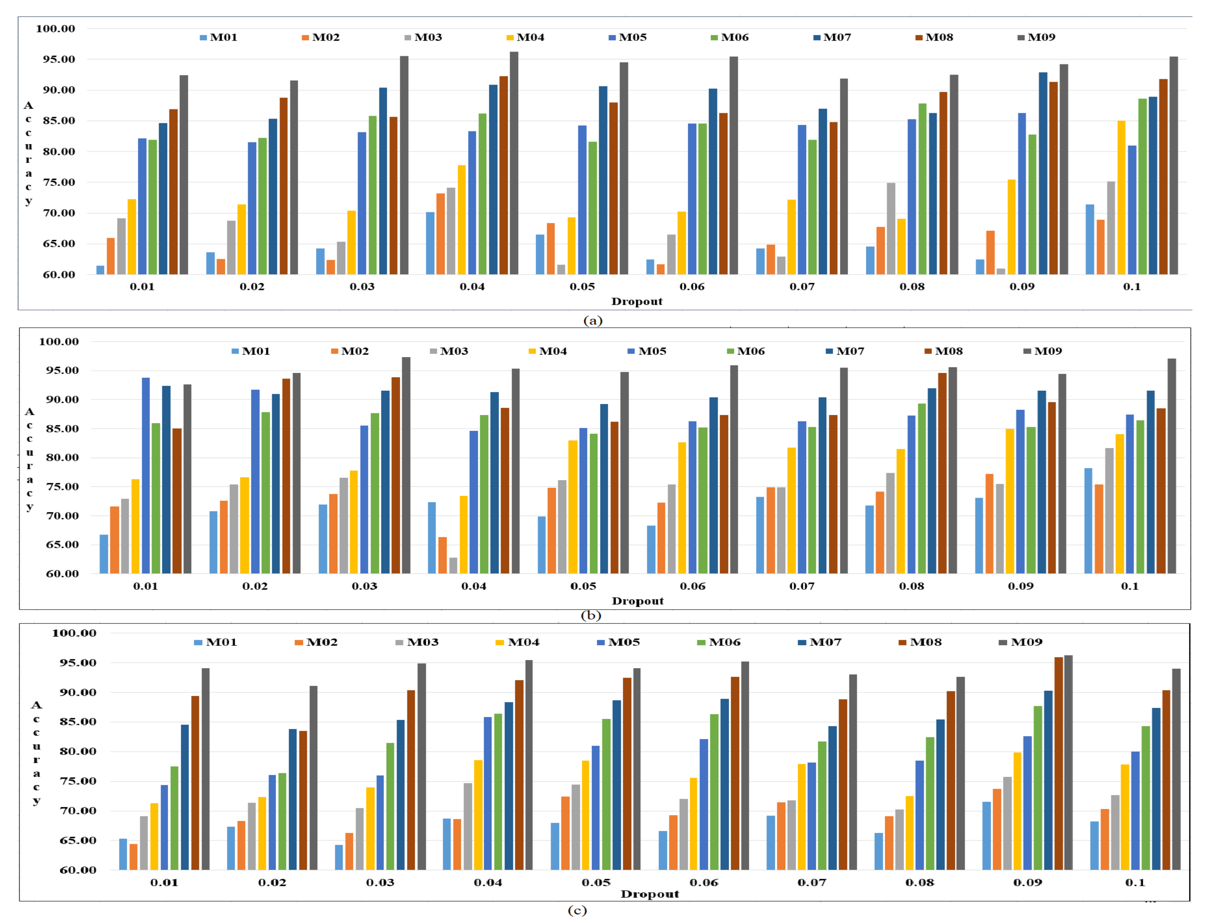
Figure 4a–c depict the average performance accuracy results for all of the models for the three datasets. Figure 4a shows the average performance accuracy results for an embedding size of 200 and with dropout rates ranging from 0.01 to 0.10. Figure 4b shows the average performance accuracy results for an embedding size of 300 and with the dropout rates ranging from 0.01–0.10. Figure 4c shows the average performance accuracy results for an embedding size of 400 and with the dropout rates ranging from 0.01 to 0.10. The experimental findings for the three datasets demonstrate that the proposed model shows effective and efficient performance over the other models, and except for very few combinations of hyperparameters, the models do not show consistent performance results.

Out of all the models under consideration, and particularly as compared models M01 and M02, when Word2Vec is applied with CNN and BiLSTM, respectively, the response of the model is very poor. If BERT is used in place of Word2Vec then some improvement can be observed in inaccuracy, which shows the effectiveness of the BERT model in text classification. The BERT model shows its supremacy over the Word2Vec model, with improvements of 5% to 10% for sentiment classification. Models M05, M06, M07, and M08 also show improvements, but the proposed model shows the highest and most consistent performance for all datasets for the embedding size of 300 and dropout rate of 0.03. Since this combination showed consistent performance for other models, the embedding size 300 and dropout rate of 0.03 were implemented on all datasets for all models to conduct further experiments, as shown in

Table 11. Hyperparameters settings.

Models	Techniques	Embedding	Activation	Embedding Size	Dropout	Optimizer	Epochs	Filters
M01	CNN	Word2Vec	ReLu	300	0.03	sgd	50	512
M02	BiLSTM	Word2Vec	ReLu	300	0.03	sgd	50	-
M03	CNN	BERT	ReLu	300	0.03	sgd	50	512
M04	BILSTM	BERT	ReLu	300	0.03	sgd	50	-
M05	MFMLSC	Word2Vec	ReLu	300	0.03	sgd	50	-
M06	MFMLSC	Word2Vec	ReLu	300	0.03	sgd	50	-
M07	MFMLSC	BERT	ReLu	300	0.03	sgd	50	-
M08	MFMLSC	BERT	ReLu	300	0.03	sgd	50	-
M09	MFMLSC	XLNet	ReLu	300	0.03	sgd	50	-

.

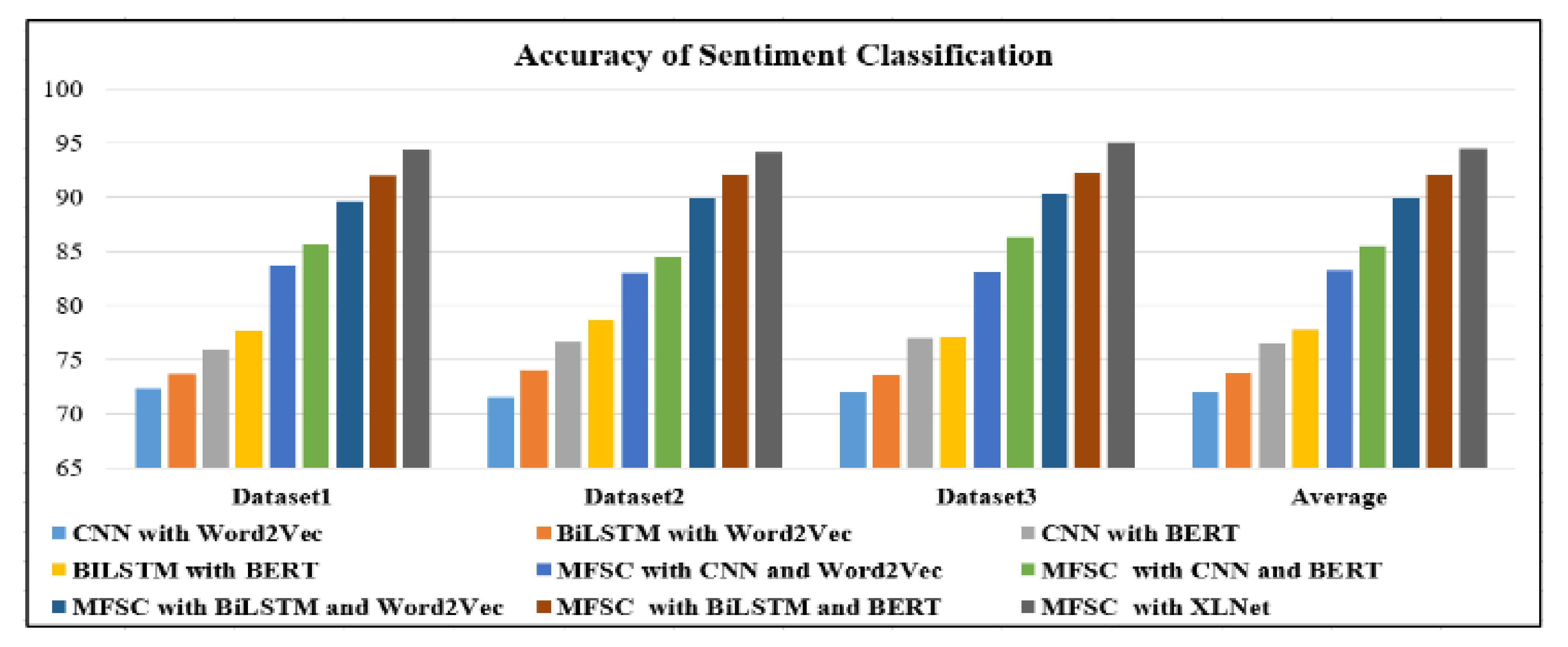
4.5. Evaluation of Multi-Fold Model of Sentiment Classification (MFSC)

To investigate the performance of a sentiment classification approach that relies solely on multi-dimensional sentiment modeling, the performance of the proposed multi-fold sentiment modeling method with XLNet (MFSC) shown in

Table 12. Sentiment classification accuracy (%) results using the MFSC model.

Methods	Dataset 1	Dataset 2	Dataset 3	Average
M01	72.36	71.53	71.98	71.96
M02	73.65	74.01	73.56	73.74
M03	75.98	76.62	77.02	76.54
M04	77.62	78.65	77.12	77.80
M05	83.65	82.98	83.12	83.25
M06	85.61	84.52	86.32	85.48
M07	89.56	89.98	90.32	89.95
M08	91.96	92.05	92.25	92.09
M09	94.32	94.1	95.01	94.48

and Figure 5 is compared with a CNN with Word2Vec, BiLSTM with Word2Vec, CNN with BERT, and BILSTM with BERT. The methods are discussed below.

CNN with Word2Vec: Firstly, Word2Vec is used to initialize the vectorized word, following which CNN is applied to extract the features of the sentiments from the dataset, and finally a fully connected network is used for sentiment classification of the social media text.

BiLSTM with Word2Vec: In this instance, Word2Vec is applied to achieve the word vectors, then BiLSTM is implemented for extraction of the sentiment characteristics of a given dataset, and finally a fully connected network is used for implement sentiment classification of the dataset.

CNN with BERT: The initialization of the word vector is accomplished with the help of BERT, then the CNN is applied for extraction of the sentiment features of the dataset, and finally a fully connected network is used for sentiment classification of the dataset.

BILSTM with BERT: Here, BERT is utilized to initialize the vector of words, followed by the BiLSTM technique being used for extraction of the sentiment features of the dataset, then in the last phase a fully connected network is used to implement sentiment classification of a dataset.

MFSM with CNN and Word2Vec: The Word2Vec, CNN, and MFSM approaches are used to classify sentiments. To begin, emoji-based symbols are treated as language symbols in a social media text. Next, Word2Vec is implemented to for the initialization of the word vector, and the CNN extracts sentiment characteristics from the dataset. Finally, the sentiment categorization approach is accomplished through a completely connected network.

MFSM with CNN and BERT: the BERT, CNN, and MFSM approaches are used to create a sentiment classification system. To begin, both language symbols and emoticon symbols are handled in datasets in the same manner as language symbols. Next, BERT is used for the initialization of the word vector, and the CNN is implemented to extract the emotional components of the dataset. Finally, the sentiment categorization approach is accomplished through a completely connected network.

MFSM with BiLSTM and Word2Vec: The Word2Vec, BiLSTM, and MFSM-based sentiment categorization approaches are used. To begin, all symbols in a dataset, including language symbols and emoticon symbols, are regarded as language symbols. The vector of the word is then initialized using Word2Vec, and the BiLSTM model extracts features of sentiments from the dataset. Finally, the sentiment categorization approach is accomplished through a completely connected network.

MFSM with BiLSTM and BERT: This is a sentiment categorization approach based on the BERT, BiLSTM, and MFSM models. To begin, in the dataset, language symbols and emoticon symbols are both treated as language symbols. The BiLSTM model collects sentiment characteristics from the dataset after initializing the word vector with BERT. Finally, a completely connected network is used to achieve sentiment categorization.

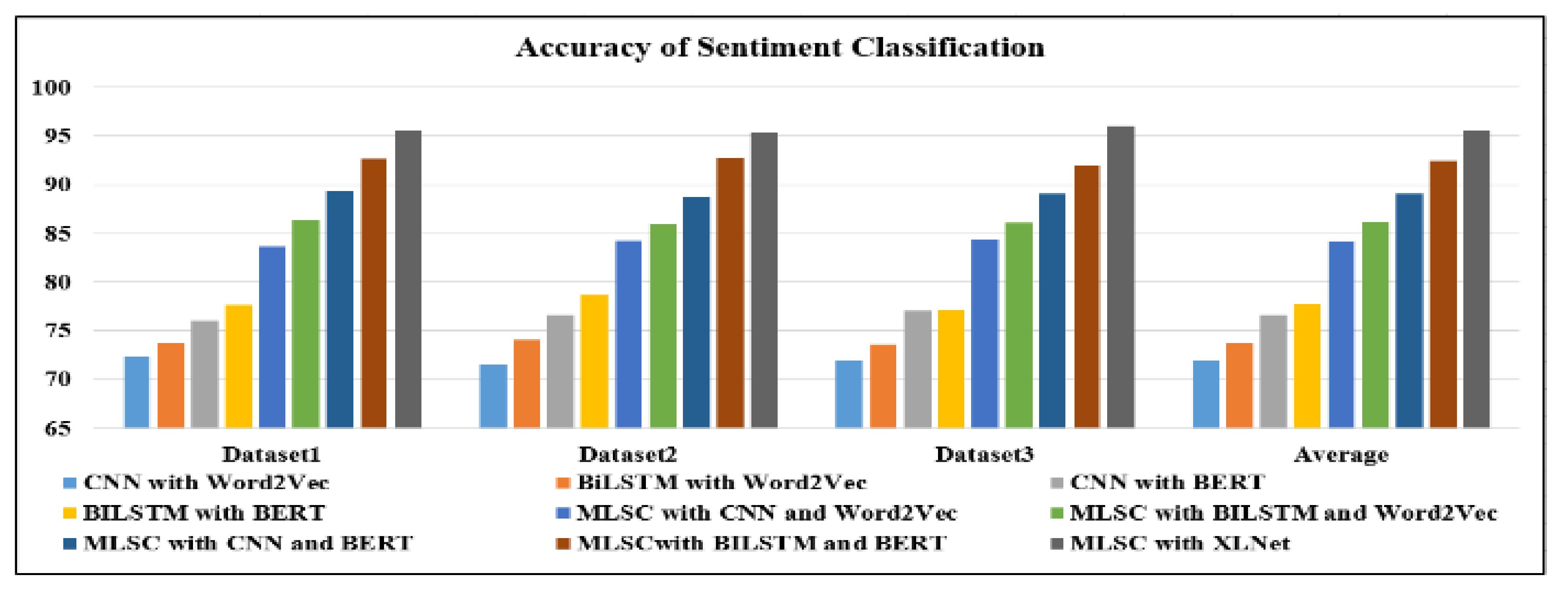
4.6. Evaluation of Multi-Level Model of Sentiment Classification (MLSC)

In the second phase of the performance evaluation of the proposed model, the evaluation is conducted only with the multi-dimension model of sentiment classification (MLSC). The MDSC model with XLNet is compared with the CNN with Word2Vec, BiLSTM with Word2Vec, CNN with BERT, and BILSTM with BERT approaches, as shown in

Table 13. Sentiment classification accuracy results using the MLSC.

Methods	Dataset 1	Dataset 2	Dataset 3	Average
M01	72.36	71.53	71.98	71.96
M02	73.65	74.01	73.56	73.74
M03	75.98	76.62	77.02	76.54
M04	77.62	78.65	77.12	77.80
M05	83.65	84.21	84.32	84.06
M06	86.33	85.98	86.1	86.14
M07	89.32	88.75	89.1	89.06
M08	92.62	92.78	91.92	92.44
M09	95.51	95.32	95.98	95.60

and Figure 6. In addition to these models, the MDSC model is also implemented with the abovementioned techniques.

MLSC with CNN and Word2Vec: The classification of sentiments is accomplished with the assistance of the Word2Vec, CNN, and MLSM models. Initially, the vectorized word is populated with the help of Word2Vec, and then with a CNN-based attention mechanism, the emotional characteristics of the dataset are retrieved from different levels of words, sentences, and phrases. Lastly, the completely linked network is used to implement the sentiment classification.

MLSC with BILSTM and Word2Vec: This is a Word2Vec, BiLSTM, and MDSC-based sentiment categorization algorithm. Here, Word2Vec is used to initialize the word vector, and then BiLSTM is used to extract sentiment features of the dataset from different levels of words and sentences using an attention mechanism. Finally, the completely linked network is used for sentiment classification in the given dataset.

MLSC with CNN and BERT: This is a BERT, CNN, and MDSC-based sentiment classification approach. The word vector’s initialization is achieved using BERT, and then the CNN is utilized to extract the sentiment features of the dataset from different levels, as discussed using an attention mechanism. Finally, the completely linked network is used for the sentiment classification of the dataset.

MLSC with BILSTM and BERT: This is a BERT, BiLSTM, and MDSC-based sentiment classification approach. BERT is used to initialize the word vector, and then BiLSTM is utilized to extract the sentiment features of the dataset from the given levels using an attention mechanism. In the final phase, using a fully interconnected computer network, the dataset classification process is carried out

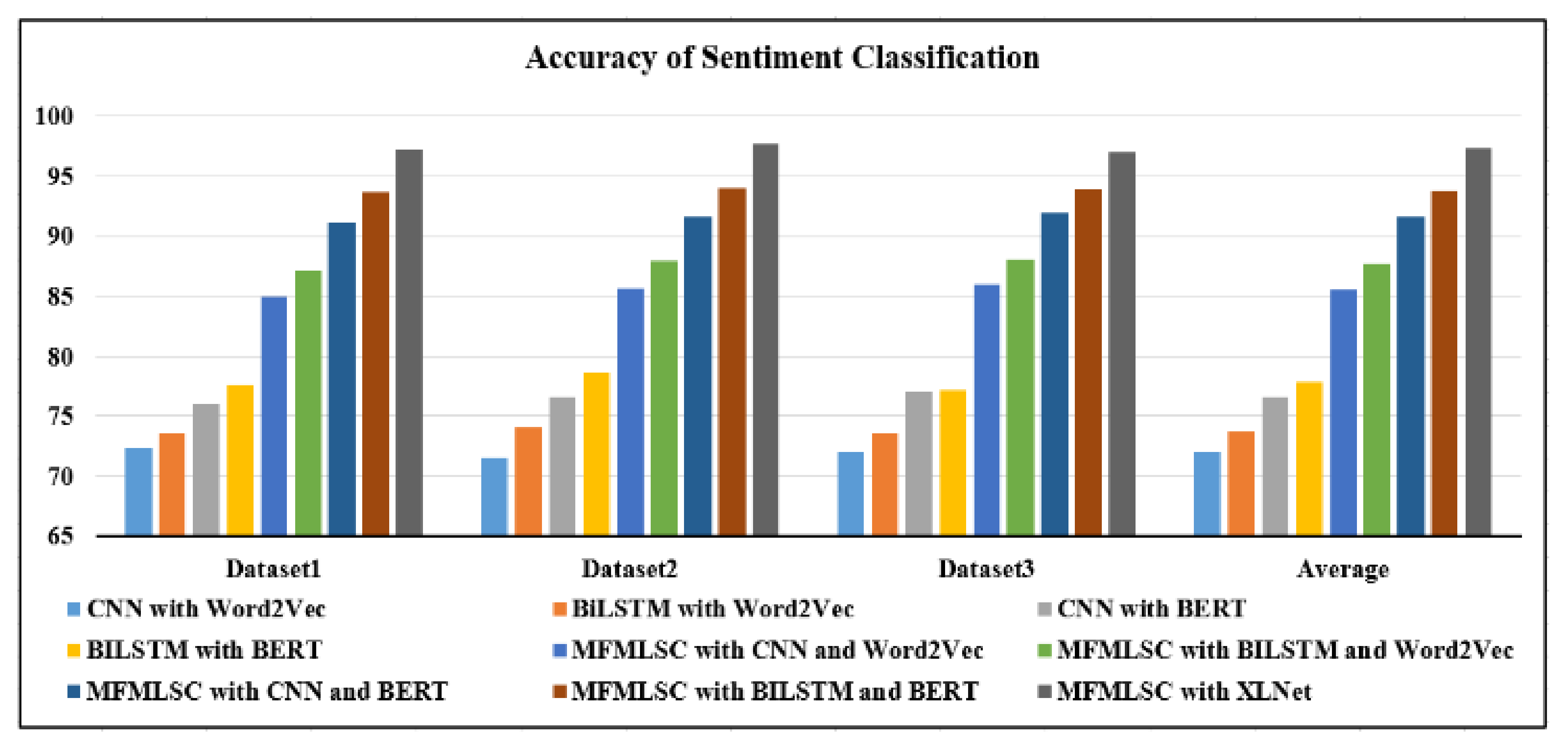
4.7. Assessment of Multi-Fold and Multi-Level Modeling of Sentiment Method (MFMLSC)

To assess our method’s overall performance, the performance results in terms of the multi-fold and multi-level classification for the sentiment method are compared with the methods discussed in the previous section.

As shown in Figure 7 and

Table 14. Accuracy results for sentiment classification using the MFMLSC.

Methods	Dataset 1	Dataset 2	Dataset 3	Average
M01	72.36	71.53	71.98	71.96
M02	73.65	74.01	73.56	73.74
M03	75.98	76.62	77.02	76.54
M04	77.62	78.65	77.12	77.80
M05	84.92	85.63	86.01	85.52
M06	87.16	87.9	88.1	87.72
M07	91.21	91.56	92.01	91.59
M08	93.63	94.01	93.9	93.85
M09	97.23	97.65	97.01	97.30

, the proposed model achieves the maximum performance as compared to the other deep learning models that use combinations of different deep learning and word embedding models. For the embedding size of 300 and dropout rate of 0.03, the proposed MFMLSC shows the highest accuracy rates during sentiment classification, with scores of 97.23%, 97.65%, and 97.01% for datset 1, dataset 2, and datset 3, respectively. The proposed model outperforms the other models, with an average accuracy rate of 97.30%.

5. Conclusions

We observed that the autoregressive-based model for sentiment classification that uses the pre-trained word vector XLNet showed the greatest classification accuracy, with an average of 97.30% accuracy for all datasets. The proposed model solved the problem of the lack of semantic information in reviews, which affects the accuracy during classification. The experimental findings demonstrated that when compared to the current methods, our method significantly increases the accuracy of the sentiment classification process for social media datasets.