Article

Hydrological Drought Frequency Analysis in Water Management Using Univariate Distributions

by
Cristian Gabriel Anghel
and
Cornel Ilinca
*
Faculty of Hydrotechnics, Technical University of Civil Engineering Bucharest, 020396 Bucharest, Romania
*
Author to whom correspondence should be addressed.
Appl. Sci. 2023, 13(5), 3055; https://doi.org/10.3390/app13053055
Submission received: 9 February 2023 / Revised: 24 February 2023 / Accepted: 24 February 2023 / Published: 27 February 2023
(This article belongs to the Special Issue Hydrology and Water Resources)

Abstract

:
The study of extreme phenomena in hydrology generally involves frequency analysis and a time series analysis. In this article we provide enough mathematics to enable hydrology researchers to apply a wide range of probability distributions in frequency analyses of hydrological drought. The article presents a hydrological drought frequency analysis methodology for the determination of minimum annual flows, annual drought durations and annual deficit volumes for exceedance probabilities common in water management. Eight statistical distributions from different families and with different numbers of parameters are used for the frequency analysis. The method of ordinary moments and the method of linear moments are used to estimate the parameters of the distributions. All the mathematical characteristics necessary for the application of the eight analyzed distributions, for the method of ordinary moments and the method of linear moments, are presented. The performance of the analyzed distributions is evaluated using relative mean error and relative absolute error. For the frequency analysis of the annual minimum flows, only distributions that have a lower bound close to the annual minimum value should be used, a defining characteristic having the asymptotic distributions at this value. A case study of hydrological drought frequency analysis is presented for the Prigor River. We believe that the use of software without the knowledge of the mathematics behind it is not beneficial for researchers in the field of technical hydrology; thus, the dissemination of mathematical methods and models is necessary. All the research was conducted within the Faculty of Hydrotechnics.

1. Introduction

Drought is a complex phenomenon and can have various approaches. Based on Wilhite and Glantz [1], Tallaksen and van Lanen [2], usually different types of droughts are distinguished, such as meteorological drought, soil moisture drought, hydrological drought and socio-economical drought. In general, drought analysis is based on drought indices (Standardized Precipitation Index, Effective Drought Index, Streamflow Drought Index, Surface Water Supply Index, etc.) or drought frequency analysis. Matalas defines drought as an extended period of dryness, and drought analysis should be performed according to magnitude and duration [3]. Mehmet defines drought “as a natural disaster that occurs when precipitation is significantly less than its normal time” [4].
The objective of this article is the frequency analysis of hydrological drought, important in the management of water resources, in the context of economic development, but also of climate change. According to A. F. Van Loon [5], hydrological drought is defined as “a lack of water in the hydrological system, manifesting itself in abnormally low streamflow in rivers and abnormally low levels in lakes, reservoirs, and groundwater”.
In this article we analyze hydrological drought represented by water deficit which is characterized by minimum flows, duration of drought and volume of water deficit. They are defined according to various thresholds generally chosen as fractions of monthly average flows or values from the duration curve of daily average flows [6,7,8,9].
The Romanian methodology regarding the analysis of minimum flows is usually carried out by extracting some data from the duration curve of average daily flows or minimum monthly flows. Another methodology is statistical processing to obtain insurance curves for the minimum annual flows, volumes and durations of the annual deficit [3,10], but it is not yet implemented in Romania, and there is no standard regarding their statistical determination.
International methodology recommends performing statistical analyses using the minimum data of the 1-day, 7-day and 30-day moving-average chronological series of minimum annual flows [3,7,9]. For proper analysis, droughts are also defined by other variables, namely durations and deficit volumes. Thus, a statistical analysis of these variables is required. In water management, durations and annual cumulative volumes are important. The time series of these two variables, resulting from the imposition of thresholds, may contain many zero values. This aspect leads to the need to use the conditional probability model [7,11,12].
In water management, the statistical analysis of the water deficit is important for the management of water resources, including the improvement of the ecological state of rivers. In Romania, until the year 2020, flow requirements of aquatic ecosystems represented the flow with a duration of 95% of the duration curve of average daily flows. The new legislation, H.G. 148/2020 [13], chooses to define periods of drought with the maximum value between the minimum monthly mean discharge with a 95% probability of occurrence and the lowest value among the monthly ecological flows; this leads in many cases to flows much lower than those before 2020. For example, for a multitude of rivers in protected areas (Porumbacu, Sambata, Vistisoara, Uz, …), the values based on the new methodology affect the hydromorphological indicators [14] that characterize the good ecological condition of rivers for most of the year, constituting a real threat to the environment.
The Faculty of Hydrotechnics, following hydrological research, started a procedure of statistical analysis of the minimum flows using a multitude of statistical distributions but also mathematical methods for determining periods of hydrological drought, being part of more extensive research regarding the correction of the ecological flow legislation.
Water deficit analysis was performed for calendar-year periods, as the use of a hydrological-year period is relevant to the water balance period but interrupts drought periods. Seasonal analysis of drought is not appropriate, because the freezing period leads to hydrological droughts smaller in magnitude and less important in water management, because there is not much water consumption, mainly only hydropower being critical. Through the annual summation of drought periods, water deficit analysis proves useful in water management decisions.
Probability distributions with three and five parameters are presented in this article, for the first time, in the statistical analysis of hydrological drought. In other materials [7,8,9,10], the Pearson III, Pearson V, log-normal, GEV, Frechet, Weibull, LogLogistic, etc., distributions are recommended for the frequency analysis of hydrological drought, especially of the minimum annual flows, all of which are three-parameter distributions. Pearson III, Pearson V, log-normal, and Weibull distributions are used in this article. In addition, the three-parameter distributions, Wilson–Hilferty and fatigue lifetime, and the five-parameter Wakeby and lambda distributions are used. Based on [7,8,9,10], in the case of perennial rivers, only statistical distributions that have a positive lower bound should be used for frequency analysis, all being three-parameter distributions and applied with the MOM or maximum likelihood parameter estimation method. Thus, it is required that the frequency analysis be performed using the L-moments parameter estimation method, which is much more stable, and that distributions of at least four parameters be used. It is recommended to use some distributions that still have a lower bound that is not only positive, but also very close to the minimum value recorded.
The methods for estimating the parameters of the presented distributions are MOM and L-moments [15]. The use of some software in hydrology limits the user’s freedom of choice, but, above all, it distances the user from understanding the phenomenon. The elimination of these inconveniences requires the detailed presentation of the distributions used and the equations for estimating the parameters of the distributions for the two methods. Other novel elements are also presented, such as the presentation of some distributions which have received very little attention in hydrology, the expressions of the quantiles of some distributions, parameter approximation relations, and frequency factors for estimating the quantile with MOM and L-moments (Appendix A). The estimation of the parameters leads to the solution of some systems of nonlinear equations, often having the integral operator, so it was necessary to obtain approximation relations of the parameters to some probability distributions. For this, approximation tests were carried out, based on [16], with polynomial, exponential or rational functions. In some cases, the variable function by which the parameter is approximated is a logarithm. The relative approximation errors of the parameters are below 10−3. For some distributions, no approximation relations were calculated because the skewness depends on two parameters, resulting in a function of two variables with poor results. For these, numerical methods were used to solve systems of equations.
Thus, all these novelty elements for these distributions presented in Table 1 will help hydrology researchers to use these distributions easily.
The fatigue lifetime and Wilson–Hilferty distributions are used for the first time in the frequency analysis of hydrological drought.
In the research carried out in the Faculty of Hydrotechnics, other distributions were also analyzed (four-parameter Johnson SU, Kappa, Burr and Kumaraswamy distributions) but the results were unsatisfactory. For transparency and to verify the results obtained, the equations necessary to apply these distributions as well as the results obtained after the frequency analysis based on the case study are presented in Tables S1–S4, Fgure S1 in the supplementary material.
The objective of the article is the presentation of rigorous criteria for the methodology for performing a frequency analysis of hydrological drought, by detailing the data selection criteria, the presentation of all the elements of the distributions, and the methods of estimating their parameters recommended in the frequency analysis of hydrological drought. Since in Romania there is no norm regarding hydrological drought, this article aims to provide the methodological basis aligned with current concerns. Modern water management principles are presented for the hydrological characteristics and particularities of Romania.
The article is organized as follows. The description of methodology, the statistical distributions by presenting the density function, the complementary cumulative function and the quantile function are found in Section 2.1. The presentation of the relations for exact calculation and the approximate relations for determining the parameters of the distributions are found in Section 2.2. Case study of hydrological drought frequency analysis for the Prigor river is in Section 3. Results, discussions and conclusions are in Section 4 and Section 5.

2. Methodology

The data analysis period must be at least the World Meteorological Organization (WMO) reference period [17].
In general, low flow frequency analysis is performed for values of the minimum annual flows (AM), the values being the minimum flows recorded in one day of a year [3,10]. In water management, data on the water deficit is of more interest, being a series of minimum 7-day low flows or minimum 30-day low flows, both of which are moving-average daily annual discharges. The 7-day time period eliminates the effect of daily fluctuations [
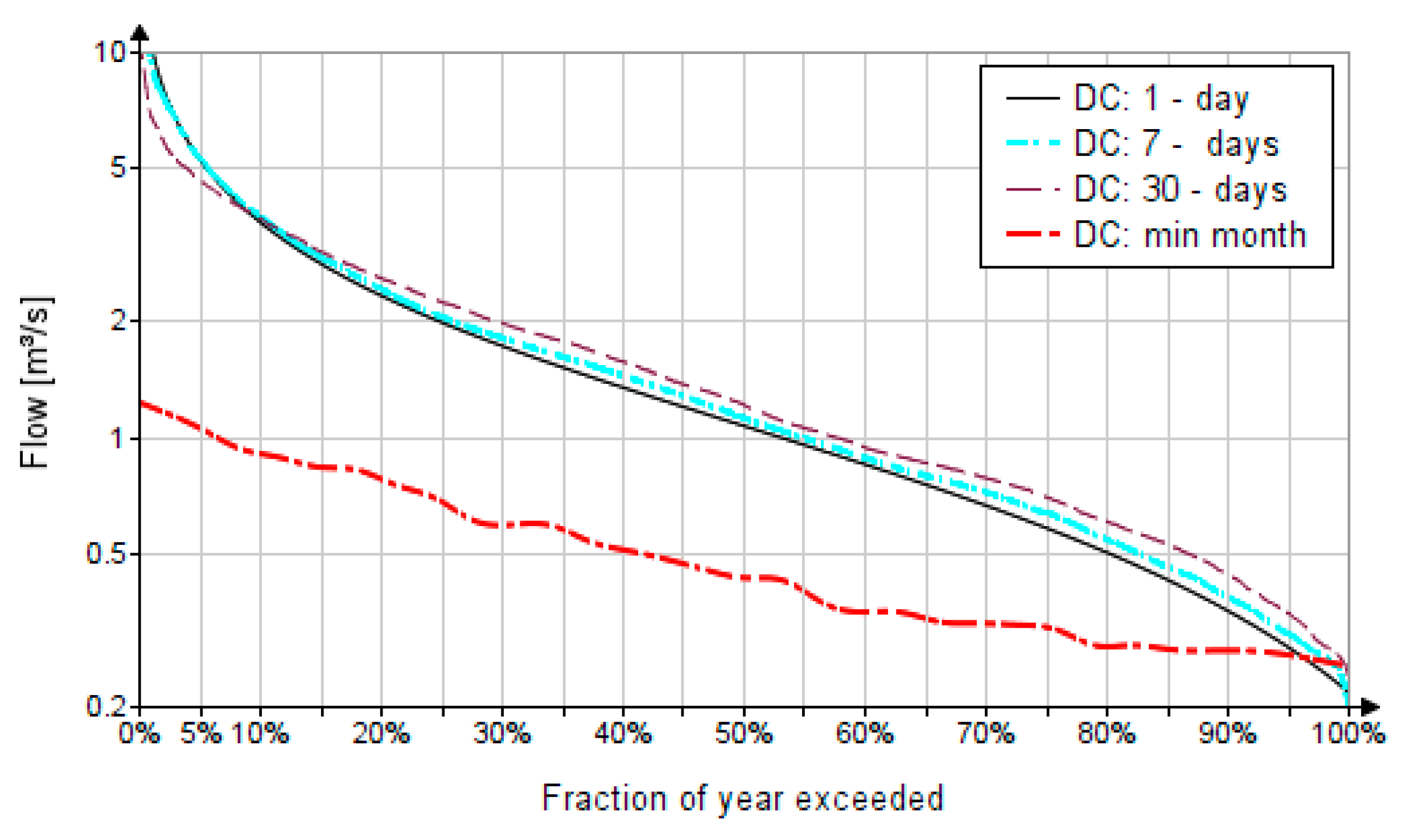
3], being useful for run-of-river facilities, and the 30-day time period is useful for dams with water reservoirs. The analysis was performed for the three variables, namely minimum 1-day low flows, minimum 7-day low flows, and minimum 30-day low flows. These values are obtained from the chronological series of daily flows observed over the entire analysis period, by selecting minimum 1-day low flows, minimum 7-day-moving-average low flows, and minimum 30-day-moving-average low flows. Figure 1 shows the duration curves used in establishing the thresholds that define hydrological drought.
These values represent the magnitude of the drought, but a drought is defined as an extended period of dryness, so in addition to the magnitude presented, the duration is also necessary [3,6]. The duration is obtained using thresholds that define the drought period. These thresholds are obtained from the duration curve of average daily flows. Usual values of thresolds are 80%, 90% and 95% of the duration curve [
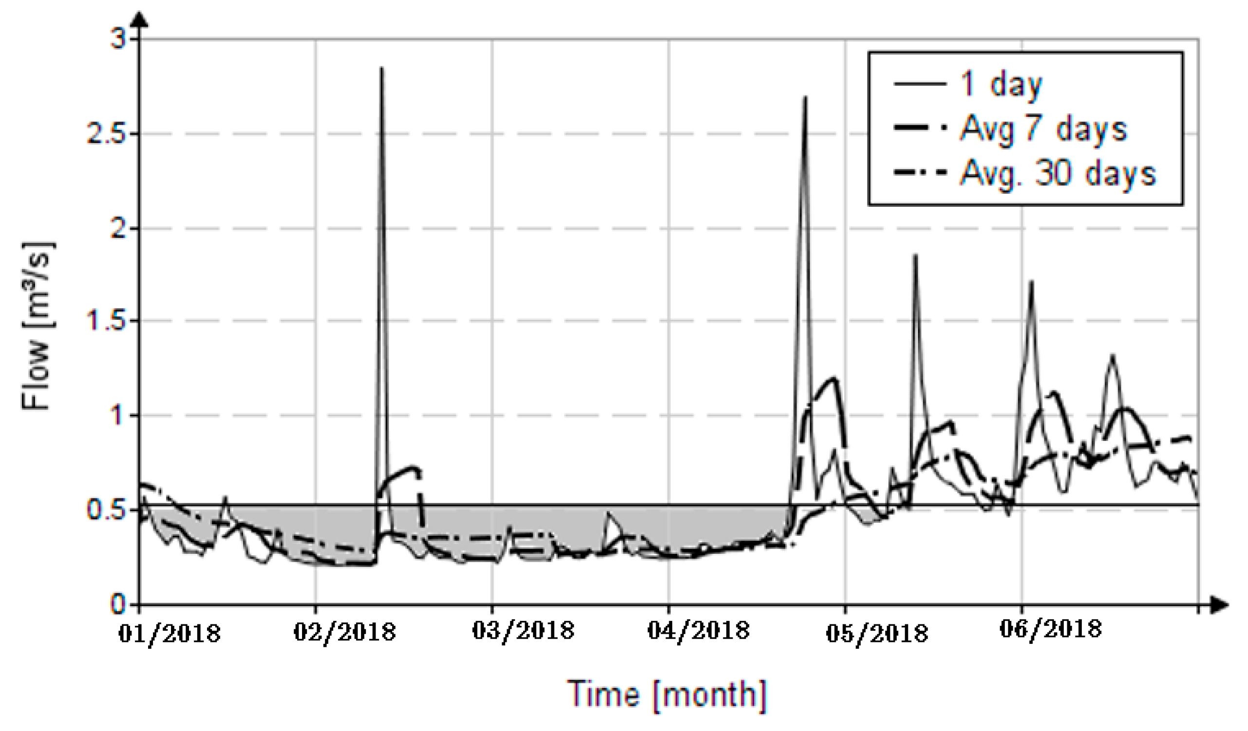
6]. With the help of these thresholds, the cumulative annual drought durations and annual volumes can be determined (Figure 2).
The duration curve of average daily flows can be approximated with a polynomial having logarithmic terms of the duration (d) and flow (k = Q/Qm) as follows:
k d = i = 1 n p + 1 C i ln d i 1
D k = exp j = 1 n k + 1 C j k j 1
If the duration curve is tabulated, cubic spline interpolation can also be used.
The determination of the volumes for the thresholds (80%, 90% and 95%) is achieved by the annual summation of the threshold differences and time series (of daily average flows, 7-day moving average, 30-day moving average). Figure 2 shows how to determine the drought volume for the time series of average daily flows corresponding to the Q80% threshold.
The duration is determined by the annual summation of the days that have values of the chronological series lower than the established thresholds.
A problem with extreme drought events is the much longer duration of low flow compared to the duration of other extreme values, such as floods. Moreover, if in floods there is a form of the flood that can be simplified (flood hydrograph), in droughts, a valid hydrograph cannot be obtained for these types of events; only recession curves are obtained (lack of precipitation). The complexity of the drought phenomenon compared to other hydrological phenomena is noticeable; it requires various types of analyses.
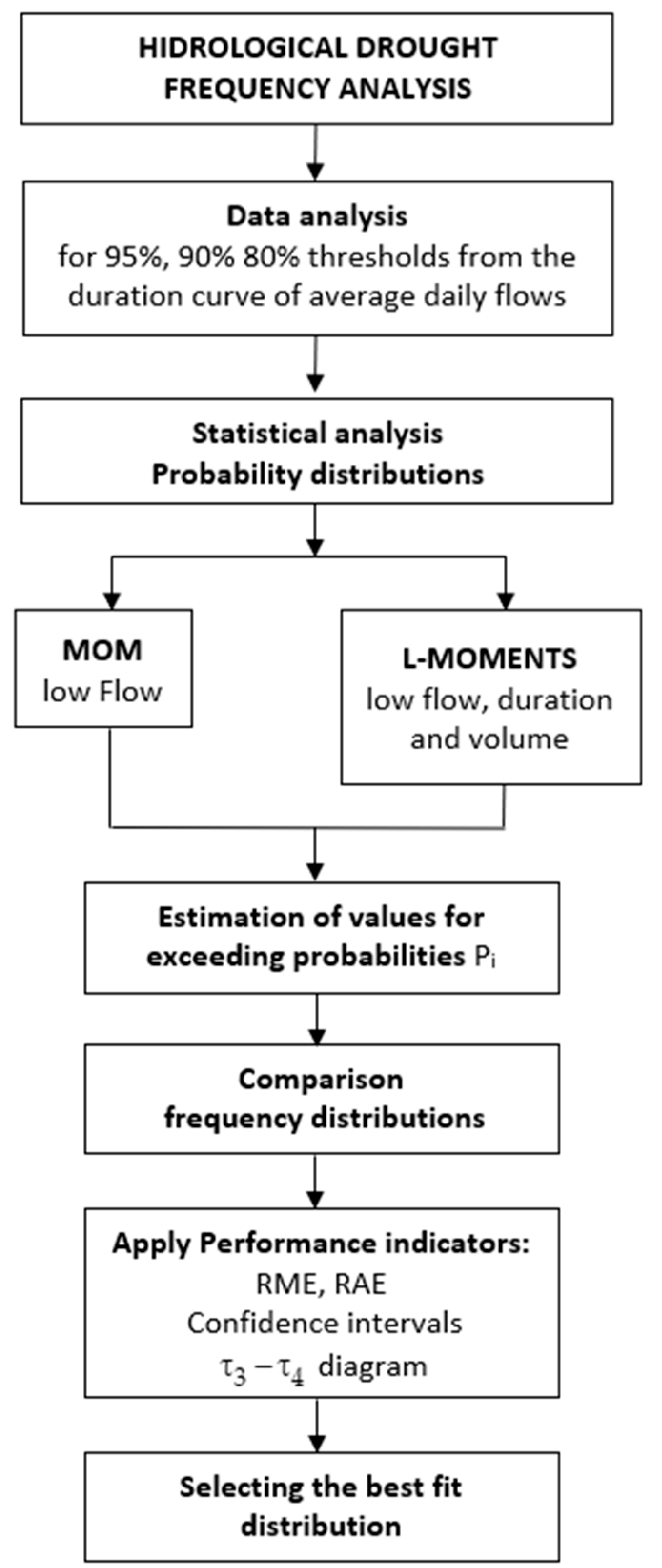
In this article, only frequency analysis will be analyzed for minimum annual flows, durations and annual deficit volumes. The analysis is carried out according to Figure 3.
For the study of hydrological drought, the time series of average daily flows and annual minimum flows are used. The chronological series of moving averages (7-day moving average, 30-day moving average) are obtained from the time series of daily average flows through moving averaging.
From the time series of average daily flows, the duration curve of average daily flows is obtained by descending ordering. The thresholds for hydrological drought analysis (80%, 90%, 95%) are extracted from the duration curve of average daily flows.
The annual deficit volumes corresponding to the three thresholds are obtained from the time series by daily summation of the volumes lower than the chosen threshold.
The annual drought durations corresponding to the three thresholds are obtained from the time series by summing the days with flows lower than the chosen threshold. These annual data represent the statistical data for frequency analysis.
In the frequency analysis of low flow, when the observed values are lower than 100 values, a correction of the skewness coefficient ( C s ) is necessary to estimate the parameters with MOM [11,18,19,20,21].
In Romania, for the low flow frequency analysis, the skewness coefficient is established according to the perennial/ephemeral character of the river. The skewness coefficient of the flows is established based on the coefficient of variation of the minimum annual flows by multiplying with a coefficient C v , depending on the perennial/ephemeral character of the river, chosen as follows [22,23,24]:
-
3 for rivers with strong supply from the aquifer;
-
2 for rivers that never dry up and with a significant supply from the aquifer in periods of low water;
-
1.5 for rivers with a deficient supply from the aquifer and with a strong trend of decreasing flows;
-
0–1 in the case of rivers that dry up (small rivers, without water supply).
This method for the calculation of the corrected skewness is an outdated method, needing an update by aligning with modern norms and methodologies. A solution is the use of the L-moments method for estimating the parameters of statistical distributions, knowing that this estimation method is more stable and less influenced by the small lengths of the observed data [15,16,17,18,19,25,26,27].
To estimate the parameters with MOM, for some three-parameter distributions, the L-moments method can be used to obtain an equivalent skewness. This involves the calculation of the shape parameter for each distribution using the L-moments method, and this will substitute the shape parameter from the MOM, obtaining the skewness, for the C s / C v ratio. This method preserves the mean and coefficient of variation of the observed data. This skewness estimation method is better than the arbitrary choice, many times, of the flow genesis function.
The use of MOM with skewness determined from L-moments is useful for a period of transition from MOM to L-moments in Romania, because the interpretation of the C s / C v ratio is well known. For the application of this method, the equivalence relations of the C s / C v ratio according to τ 3 are presented in Table A2 from Appendix C.
For frequency analysis of the annual volume deficit and duration, due to the fact that the data can contain zero values, it is necessary to use a conditional probability model [3,11,28]. The same model is recommended for application in the statistical analysis of annual low flows when the observed data contains zero values (rivers that dry up). This model assumes a correction of the cumulative function and the quantile of the analyzed distribution, as follows:
F x * = 1 p 0 F x
x p * = 0 , p > F 0 * x p 1 p 0
where p 0 is the empirical probability from which the values are zero.
The next section presents the theoretical distributions analyzed in the research of the Faculty of Hydrotechnics regarding the regionalization studies of the low flows in Romania.
The inverse forms of the distributions (quantile functions) can be expressed both for MOM and for L-moments with the frequency factor.
The frequency factors of the analyzed distributions are presented in Appendix A.

2.1. Probability Distributions

The probability density function, f x , the complementary cumulative distribution function, F x , and quantile function, x p , for analyzed distributions are:

2.1.1. Log-Normal (LN3)

It represents one of the most used statistical distributions in hydrology. The three-parameter log-normal distribution (LN3) is a generalized form of the two-parameter log-normal distribution (LN2), with x shifted by a position parameter that characterizes the lower bound [18,20,21,29].
f x = exp ln x γ α 2 2 β 2 x γ β 2 π
F x = 1 1 2 e r f 1 2 β ln x γ α + 1
x p = F 1 x = γ + exp α + β q n o r m 1 p , 0 , 1 = γ + q l n o r m 1 p , α , β
where α , β , γ are the shape, the scale, and the position parameters, respectively; x can take any values of range γ < x < .

2.1.2. Pearson III (PE3)

The Pearson III represents a generalized form of the two-parameter gamma distribution and a particular case of the four-parameter gamma distribution [18,20]. It represents the parent distribution in Romania in statistical analysis in hydrology [30,31].
f x = x γ α 1 β α Γ α exp x γ β = 1 β d g a m m a x γ β , α
F x = 1 γ x f x d x = 1 1 β Γ α γ x x γ β α 1 exp x γ β d x = Γ α , x γ β Γ α
x p = γ + β q g a m m a 1 p , α
where α , β , γ are the shape, the scale, and the position parameters, respectively, and x can take any values of range γ < x < if β > 0 , or < x < γ if β < 0 and α > 0 ; μ , σ represent the mean (expected value) and standard deviation. If β < 0 (negative skewness), then the first argument of the inverse of the distribution function gamma, Γ 1 1 p ; α becomes Γ 1 p ; α .
The built-in function from Mathcad, q g a m m a 1 p , α = γ 1 1 p Γ α , α , returns the inverse cumulative probability distribution for probability p, for the gamma distribution, where γ 1 is the inverse of the lower incomplete gamma function [32].

2.1.3. Pearson V (IPV)

The Pearson V distribution represents the inverse of the Pearson III distribution [3,20].
f x = exp β x γ β Γ α 1 x γ β α
F x = Γ α 1 , β x γ Γ α 1
x p = γ + β Γ 1 p ; α 1 = γ + β q g a m m a p , α 1
where α , β , γ are the shape, the scale, and the position parameters, respectively; α , β > 0 ; γ < x min , and x can take any values of range γ < x < .

2.1.4. Wilson–Hilferty (WH3)

The three-parameter Wilson–Hilferty distribution is a generalized form of the two-parameter Wilson–Hilferty distribution. Both are cases of Amoroso distribution [20,29].
f x = 3 exp x γ β 3 β Γ α x γ β 3 α 1
F x = 1 γ x 3 exp x γ β 3 β Γ α x β 3 α 1 d x = Γ α , x γ β 3 Γ α
x p = γ + β q g a m m a 1 p , α 3
where α , β , γ are the shape, the scale, and the position parameters, respectively; α , β > 0 ; x can take any values in the range γ < x < .

2.1.5. Fatigue Lifetime (FL3)

This distribution is also known as the Birnbaum–Saunders distribution [33].
f x = 1 + x γ β 2 α x γ 3 β exp β x γ 1 2 2 x γ α 2 β 2 π
F x = 1 γ x 1 + x γ β 2 α x γ 3 β exp β x γ 1 2 2 x γ α 2 β 2 π d x
F x = 1 1 2 1 + e r f β x γ 1 α 2 x γ β
x p = γ + α q n o r m p , 0 , 1 2 α 2 q n o r m p , 0 , 1 2 + 4 + α 2 q n o r m p , 0 , 1 2 + 2 2 β ,   if   p 0.5
x p = γ + α q n o r m p , 0 , 1 2 α 2 q n o r m p , 0 , 1 2 + 4 + α 2 q n o r m p , 0 , 1 2 + 2 2 β ,   if   p > 0.5
where α , β , γ are the shape, the scale and the position parameters; α , β > 0 ; x can take any values in the range γ < x < .

2.1.6. Weibull (W3)

The distribution represents a particular case of the generalized extreme value distribution when the shape parameter is positive. It is also known as the Type III extreme value distribution [7,11,12,16,18,20,34].
f x = α β x γ β α 1 e x γ β α
F x = e x γ β α
x p = γ + β ln p 1 / α
where α , β , γ are the shape, the scale, and the position parameters, respectively; α , β > 0 ; x can take any values in the range γ < x < .

2.1.7. The Five-Parameter Wakeby Distribution (WK5)

The five-parameter Wakeby distribution has no form for density and cumulative function, being classified as a quantile function. The Wakeby distribution is a distribution that was introduced in the frequency analysis of extremes by Houghton [18,19,35] in order to fulfil, as much as possible, the “separation effect” described by Matalas et al. 1975 [35], namely to carry out an analysis so that the maximum flows are not influenced too much by the low flows, and vice versa. The Wakeby distribution separates the right-hand side from the left-hand side of the distribution. It has the property of a very thick left-hand tail (high flows) and a right-hand tail (low flow) thick enough to decrease the average skew, which makes the middle part of the distribution steeper than traditional skewed curves. A particular case of the five-parameter Wakeby distribution represents the Wakeby distribution of four parameters when ξ = 0 [18] and the Pareto Type II distribution when γ = 0 , or in particular cases when α β 1 p β or γ δ 1 p δ has a constant value [19].
The quantile function of WK5 distributions is [18,35]
x p = ξ + α β 1 p β γ δ 1 p δ
where α , γ are the scale parameters, β , δ are the shape parameters, and ξ is the position parameter.

2.1.8. The Five-Parameter Lambda Distribution (L5)

The five-parameter lambda distribution seems part of the same family as the Wakeby distribution, being also classified as a quantile function. It has no form for density and cumulative function. It represents a distribution of a generalization of the Tukey lambda quantile function [36] and an alternative to the Wakeby distribution to fulfil the “separation effect”. A particular case of the five-parameter lambda distribution represents the lambda distribution of four parameters when γ = 0 [36], and the Tukey distribution when λ = 0 , or in particular cases when α p β or λ 1 p δ has a constant value.
The quantile function of L5 distributions is [36]:
x p = γ + α p β λ 1 p δ
where α , λ are the scale parameters, β , δ are the shape parameters, and γ is the position parameter.

2.2. Parameter Estimation

The parameter estimation of the analyzed statistical distributions is presented for MOM and L-moments, two of the most used methods in hydrology for parameter estimation.

2.2.1. Log-Normal (LN3)

For estimation with MOM, the distribution parameters have the following expressions [37]:
α = ln σ 2 C s 2 + 4 C s 3 4 3 C s 2 + 4 C s 2 3 1 2 ln 4 3 C s 2 + 4 C s 2 3 2 C s 2 + 4 C s 3 2 + 1
β = ln 4 3 C s 2 + 4 C s 2 3 2 C s 2 + 4 C s 3 2 + 1 0.5
γ = μ σ 2 C s 2 + 4 C s 3 4 3 C s 2 + 4 C s 2 3
The parameter estimation with the L-moments method is performed numerically (definite integrals) based on the equations using the quantile of the function [19].
An approximate form of parameter estimation can be adopted.
Thus, for the estimation with the L-moments, the shape parameter β can be evaluated numerically with the following approximate forms, depending on L-skewness ( τ 3 ) [20]:
if 0 < τ 3 1 3 :
β = 4.379498 10 4 + 2.0295824 τ 3 + 0.23041762 τ 3 2 0.92166328 τ 3 3 + 3.8546644 τ 3 4 3.6560389 τ 3 5
if 1 3 < τ 3 2 3 :
β = 5.3943247 10 2 + 2.6732827 τ 3 2.9211411 τ 3 2 + 7.3388138 τ 3 3 8.1997299 τ 3 4 + 4.3299046 τ 3 5
if 2 3 < τ 3 < 1 :
β = 0.81822527 + 7.818908 τ 3 4 8.1529453 τ 3 8 + 0.1554959 τ 3 12 1 + 2.5188862 τ 3 4 4.9742123 τ 3 8 + 1.592552 τ 3 12
With parameter β known, the parameter α and the parameter γ are determined with the following expressions:
α = ln L 2 e r f 0.5 β β 2 2
γ = L 1 exp α + 0.5 β 2

2.2.2. Pearson III (PE3)

For estimation with MOM, the distribution parameters have the following expressions [17,18,19,20]:
α = 2 C s 2
β = σ 2 C s
γ = μ α β
where C s represents the skewness coefficient.
The parameter estimation with the L-moments method is performed numerically (definite integrals) based on the equations using the quantile of the function. An approximate form of parameter estimation can be adopted. Thus, for the estimation with the L-moments, the shape parameter α can be evaluated numerically with the following approximate forms, depending on L-skewness ( τ 3 ) [20]:
if 0 < τ 3 1 3 :
α = exp 3.164791927 5.108735285 ln τ 3 4.116014079 ln τ 3 2 2.985250105 ln τ 3 3 1.327399577 ln τ 3 4 0.373944875 ln τ 3 5 0.065421611 ln τ 3 6 0.006508037 ln τ 3 7 0.000281969 ln τ 3 8
if 1 3 < τ 3 2 3 :
α = exp 3.9918551 10.781466 ln τ 3 21.557807 ln τ 3 2 33.8752604 ln τ 3 3 35.0641585 ln τ 3 4 22.921163 ln τ 3 5 8.5491823 ln τ 3 6 1.3855653 ln τ 3 7
if 2 3 < τ 3 < 1 :
α = 5.17817436 26.209448756 τ 3 + 62.12494027 τ 3 2 84.39423264 τ 3 3 + 67.08589624 τ 3 4 29.150288079 τ 3 5 + 5.364968945 τ 3 6 1 + 0.0005134 τ 3 + 0.00063644 τ 3 2
The scale parameter β and the position parameter γ are determined with the following expressions:
β = L 2 π Γ α Γ α + 1 2
γ = L 1 α β

2.2.3. Pearson V (IPV)

The equations needed to estimate the parameters with MOM have the following expressions [20]:
μ = γ + β α 2
σ 2 = β 2 α 2 1 α 3 1 α 2
C s = 4 α 3 0.5 α 4
For estimation with MOM, parameter α can be evaluated numerically with the following approximate forms, depending on C s 0.2 :
α = exp 3.04183273 1.532335271 ln C s + 0.350524466 ln C s 2 + 0.114266418 ln C s 3 0.018372078 ln C s 4 0.026493586 ln C s 5 0.000919818 ln C s 6 + 0.004375959 ln C s 7 + 0.000310213 ln C s 8 0.000357638 ln C s 9
The scale parameter β and the position parameter γ are determined with the following expressions:
β = σ α 2 α 3
γ = μ β α 2
The parameter estimation with the L-moments method is performed numerically (definite integrals) based on the equations using the quantile of the function.
An approximate form of parameter estimation can be adopted. Thus, for the estimation with the L-moments, the shape parameter α can be evaluated numerically with the following approximate forms, depending on L-skewness ( τ 3 ) [20]:
α = exp 0.692740135 0.466055586 ln τ 3 + 0.460508385 ln τ 3 2 + 0.470172127 ln τ 3 3 + 0.938027763 ln τ 3 4 + 0.805363294 ln τ 3 5 + 0.359846034 ln τ 3 6 + 0.08945247 ln τ 3 7 + 0.011775528 ln τ 3 8 + 0.000641664 ln τ 3 9
The scale parameter β and the position parameter γ are determined with the following expressions [16]:
β = L 2 1 α 2 2 z
γ = L 1 β α 2
where z has the following expression:
z = exp 4.083852739 11.442833473 ln α + 10.701793287 ln α 2 6.513639901 ln α 3 + 2.527142191 ln α 4 0.640389591 ln α 5 + 0.105546499 ln α 6 0.010903032 ln α 7 + 0.000641094 ln α 8 0.000016371 ln α 9

2.2.4. Wilson–Hilferty (WH3)

The equations needed to estimate the parameters with MOM have the following expressions [20]:
μ = γ + β Γ α Γ α + 1 3
σ 2 = β 2 Γ α Γ α + 2 3 1 Γ α Γ α + 1 3 2
C s = α 3 Γ α 2 Γ α + 2 3 Γ α + 1 3 + 2 Γ α 3 Γ α + 1 3 3 Γ α + 2 3 Γ α Γ α + 1 3 2 Γ α 2 Γ α + 2 3 Γ α + 1 3 2 Γ α
The shape parameter can be obtained approximately, depending on the skewness coefficient, using the following exponential function [20]:
α = exp 1.6047146 1.2117058 ln C s 2.4627986 10 1 ln C s 2 3.0754515 10 2 ln C s 3 + 1.3529125 10 2 ln C s 4 + 5.4495596 10 3 ln C s 5 + 6.0310303 10 7 ln C s 6 3.5860178 10 4 ln C s 7 7.3564689 10 5 ln C s 8 4.7318329 10 6 ln C s 9
β = σ Γ α + 2 3 Γ α Γ α + 1 3 2 Γ α 2
γ = μ β Γ α + 1 3 Γ α
The parameter estimation with the L-moments method is performed numerically (definite integrals) based on the equations using the quantile of the function.
An approximate form can be adopted based on the parameter estimation, depending on L-skewness ( τ 3 ), as follows [20]:
if 0 < τ 3 1 / 3 :
α = exp 4.16202506 3.261604018 ln τ 3 1.783702334 ln τ 3 2 0.770946644 ln τ 3 3 0.221698815 ln τ 3 4 0.041191426 ln τ 3 5 0.004665295 ln τ 3 6 0.000287712 ln τ 3 7 0.000007207 ln τ 3 8
if 1 / 3 < τ 3 2 / 3 :
α = exp 5.264027693 9.134993593 ln τ 3 15.845477811 ln τ 3 2 19.874003352 ln τ 3 3 15.495267042 ln τ 3 4 6.752325319 ln τ 3 5 1.255615645 ln τ 3 6
if 2 / 3 < τ 3 < 1 :
α = exp 7.712526023 93.06660109 ln τ 3 1.519099681 10 3 ln τ 3 2 1.602587644 10 3 ln τ 3 4 1.041173897 10 5 ln τ 3 4 4.152482998 10 5 ln τ 3 5 9.887282 10 5 ln τ 3 6 1.287749298 10 6 ln τ 3 7 7.050767642 10 5 ln τ 3 8
β = L 2 Γ α + 1 3 Γ α 2 z
γ = L 1 β Γ α + 1 3 Γ α
where z = 0 1 q g a m m a 1 p , α 1 / 3 p d p , which can be approximated with the following equation:
z = exp 1.037385169 + 0.592727202 ln α 0.107494558 ln α 2 + 0.027616773 ln α 3 0.002977204 ln α 4 0.000546413 ln α 5 + 0.00123125 ln α 6 + 0.000420922 ln α 7 + 0.000052295 ln α 8 + 0.000002315 ln α 9

2.2.5. Fatigue Lifetime (FL3)

The equations needed to estimate the parameters with MOM have the following expressions [33]:
μ = γ + 2 + α 2 2 β
σ 2 = α 2 4 + 5 α 2 4 β 2
C s = 4 α 2 11 α 2 + 6 α 4 + 5 α 2 3
The parameter estimation with the L-moments method is performed numerically (definite integrals), based on the equations using the quantile of the function.
An approximate form can be adopted based on the parameter estimation, depending on L-skewness ( τ 3 ), as follows:
if 0 < τ 3 0.3 :
α = 0.000329932 + 2.035420236 τ 3 1 0.060182808 τ 3 1.000075667 τ 3 2 0.630055585 τ 3 3
if 0.3 < τ 3 0.7 :
α = 0.413986909 0.600184554 τ 3 1 3.179942891 τ 3 + 3.026068085 τ 3 2 0.754825029 τ 3 3
β = 1 2 L 2 0.000467677 + 1.13508777 α + 0.514463902 α 2 + 0.532996863 α 3 1 + 0.503786644 α + 0.036559683 α 2 0.005584778 α 3 + 0.000507637 α 4 0.00002505 α 5 + 0.000000515 α 6
γ = L 1 2 + α 2 2 β

2.2.6. Weibull (W3)

The equations needed to estimate the parameters with MOM have the following expressions [18,20]:
μ = γ + β Γ 1 + 1 α
σ 2 = β 2 Γ 1 + 2 α Γ 1 + 1 α 2
C s = Γ 1 + 3 α 3 Γ 1 + 2 α Γ 1 + 1 α + 2 Γ 1 + 1 α 3 Γ 1 + 2 α Γ 1 + 1 α 2 1.5
The shape parameter can be obtained approximately, depending on the skewness coefficient, using the following rational function [20]:
α = 3.5947875 3.7374529 C s + 2.7023151 C s 2 1.1835102 C s 3 + 0.4318107 C s 4 0.0042306 C s 5 + 0.0045545 C s 6 0.0046984 C s 7 1 + 0.0931316 C s 0.12783 C s 2 + 0.0671082 C s 3 + 0.1113667 C s 4 0.0425475 C s 5 + 0.0673629 C s 6 0.0157628 C s 7
β = σ Γ 1 + 2 α Γ 1 + 1 α 2
γ = μ β Γ 1 + 1 α
The equations needed to estimate the parameters with L-moments have the following expressions [18,20]:
L 1 = γ + β Γ 1 + 1 α
L 2 = β Γ 1 + 1 α 1 2 1 α
L 3 = β Γ 1 + 1 α 1 2 1 α 2 2 1 α 3 1 α 2 1 α 1 + 1
An approximate form of the shape parameters can be adopted, depending on L-skewness ( τ 3 ), as follows [20]:
α = 3.528107902 6.294082546 τ 3 + 2.767652838 τ 3 2 1 + 4.599024923 τ 3 7.993601572 τ 3 2 + 2.423742593 τ 3 3
With parameter α known, the parameters β and γ are determined with the following expressions:
β = L 2 Γ 1 + 1 α 1 2 1 α
γ = L 1 β α Γ 1 α

2.2.7. The Five-Parameter Wakeby Distribution (WK5)

The equations needed to estimate the parameters with MOM have the following expressions:
μ = ξ + α β + 1 γ δ 1
σ 2 = α 2 β + 1 2 2 β + 1 2 α γ β + 1 β + 1 δ δ 1 γ 2 δ 1 2 2 δ 1
The equations for skewness and kurtosis are presented in Appendix D.
The equations needed to estimate the parameters with L-moments have the following expressions [16,18,35,36]:
L 1 = ξ + α β + 1 + γ 1 δ
L 2 = α β + 1 β + 2 + γ 2 δ 1 δ
L 3 = γ δ + 1 1 δ 2 δ 3 δ + α 1 β β + 1 β + 2 β + 3
L 4 = γ δ + 1 δ + 2 4 δ 3 δ 2 δ 1 δ + α 2 β 1 β β + 1 β + 2 β + 3 β + 4

2.2.8. The Five-Parameter Lambda Distribution (L5)

The equations needed to estimate the parameters with MOM have the following expressions:
μ = γ β + 1 + α β + 1 λ δ + 1
σ 2 = λ 2 2 δ + 1 2 α λ Γ β + 1 Γ δ + 1 Γ β + δ + 2 + 2 λ γ β + 1 + α β + 1 λ δ + 1 δ + 1 2 γ λ δ + 1 + α 3 2 β + 1 2 α γ β + 1 + α β + 1 λ δ + 1 β + 1 + γ β + 1 + α β + 1 λ δ + 1 2 + 2 α γ β + 1 2 γ γ β + 1 + α β + 1 λ δ + 1 + γ 3
The equations for skewness and kurtosis are presented in Appendix D.
The equations needed to estimate the parameters with L-moments have the following expressions [36]:
L 1 = γ β + 1 + α β + 1 λ δ + 1
L 2 = α β β + 1 β + 2 λ δ δ + 1 δ + 2
L 3 = α β β 1 β + 1 β + 2 β + 3 + λ δ 1 δ δ + 1 δ + 2 δ + 3
L 4 = α β β 2 β 1 β + 1 β + 2 β + 3 β + 4 + λ δ 3 δ δ 2 2 δ + 1 δ + 2 δ + 3 δ + 4

3. Case Study

The presented case study consists in the determination of minimum annual flows, drought durations and annual volume deficits on the Prigor River, Romania, using the proposed methodology.
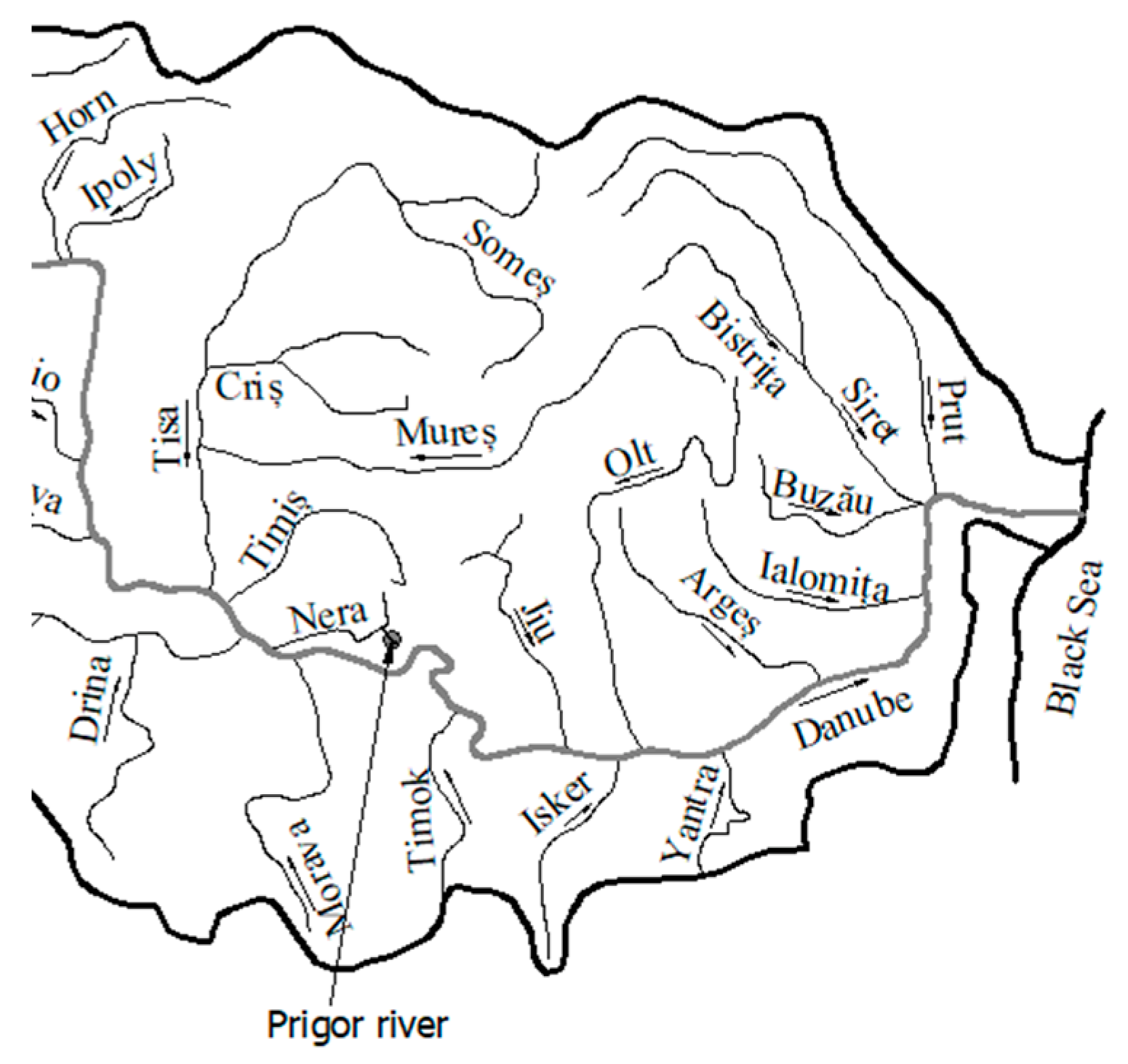
The Prigor River is the left tributary of the Nera River, and it is located in the south-western part of Romania, as shown in Figure 4.
The main morphometric characteristics of the river are presented in Table 2 [38].
In the section of the hydrometric station, the drainage area is 141 km2 and the average altitude is 729 m. The minimum 1-day data are presented in Table 3.
There are 31 annual observed data for low flows, with the values of the main statistical indicators presented in Table 4.
For parameter estimation with L-moments, the data series must be in ascending order for the calculation of natural estimators, the respective L-moments.
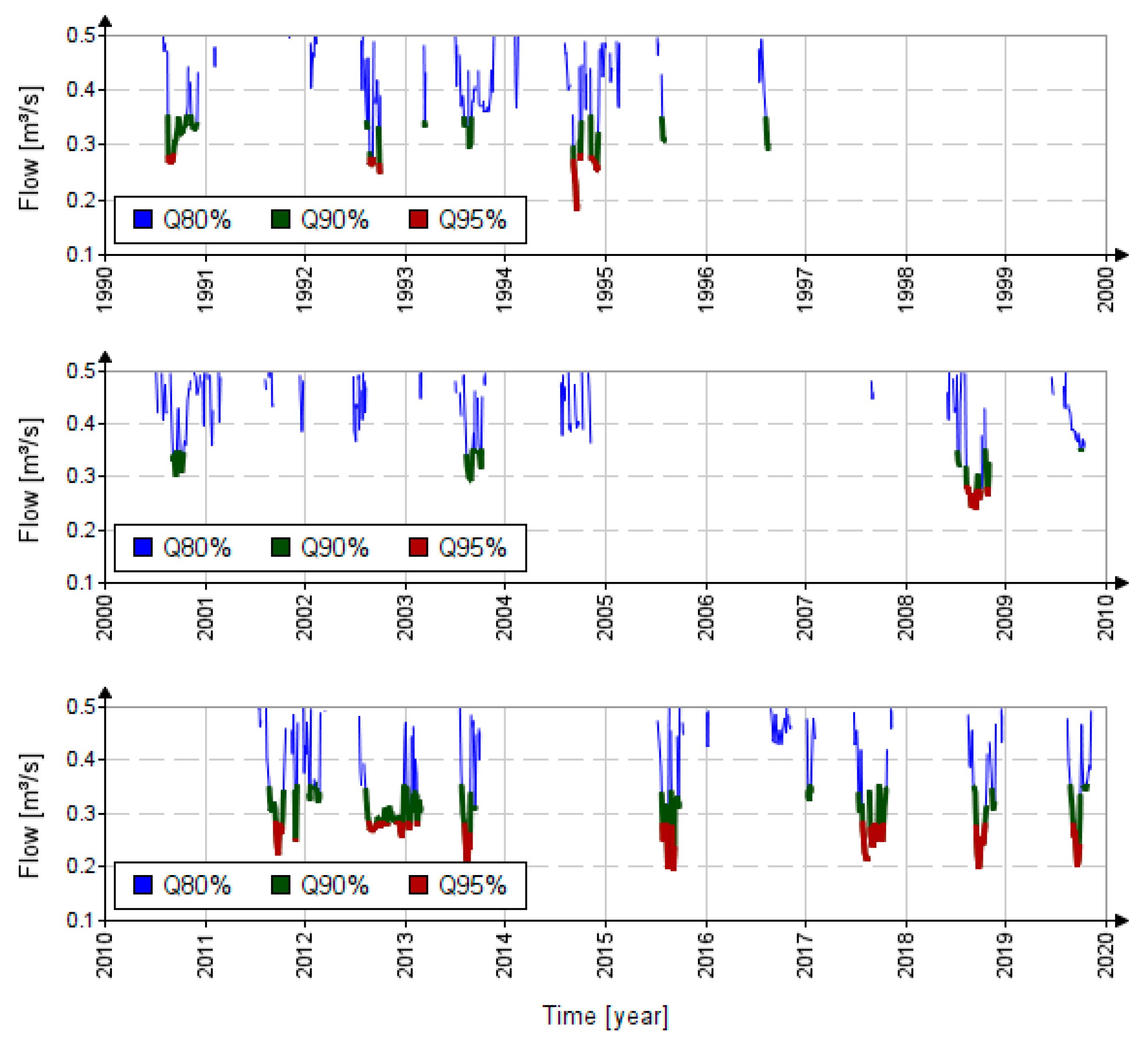
In this case study, for low-flow frequency analysis with MOM, a coefficient of 3 was chosen for the choice skewness, to reflect the perennial/ephemeral character of the river. It can be seen from Figure 5 that the predominant droughts are in the summer, and in the winter period, the important droughts appear only in 2012, 2013 being the driest year as well. The droughts of 2012 and 2013 are predominantly in the summer period, having the highest magnitude in those years.
The deficit volumes calculated for the thresholds of 95% are presented in Table 5. The analysis was also conducted for other thresholds, such as 90% and 80%.
The drought durations determined for the thresholds of 95% are presented in Table 6. The analysis was also conducted for other thresholds, such as 90% and 80%.

4. Results

The frequency analysis of hydrological drought consisted in determining the minimum flows, annual volumes and durations for exceedance probabilities used in water management [39]. Eight probability distributions, with three and five parameters, were used. The distribution parameters were estimated for MOM and L-moments for the analysis of minimum annual flows, and for L-moments for the analysis of annual volume deficits and annual drought durations.
For the analysis of minimum flows with MOM, the skewness coefficient was chosen, depending on the ephemeral/perennial character of the river. In this case, the multiplication coefficient 3, applied to the coefficient of variation of the data, was used, resulting in a skewness of 1.351, different from 1.053 of the observed values.
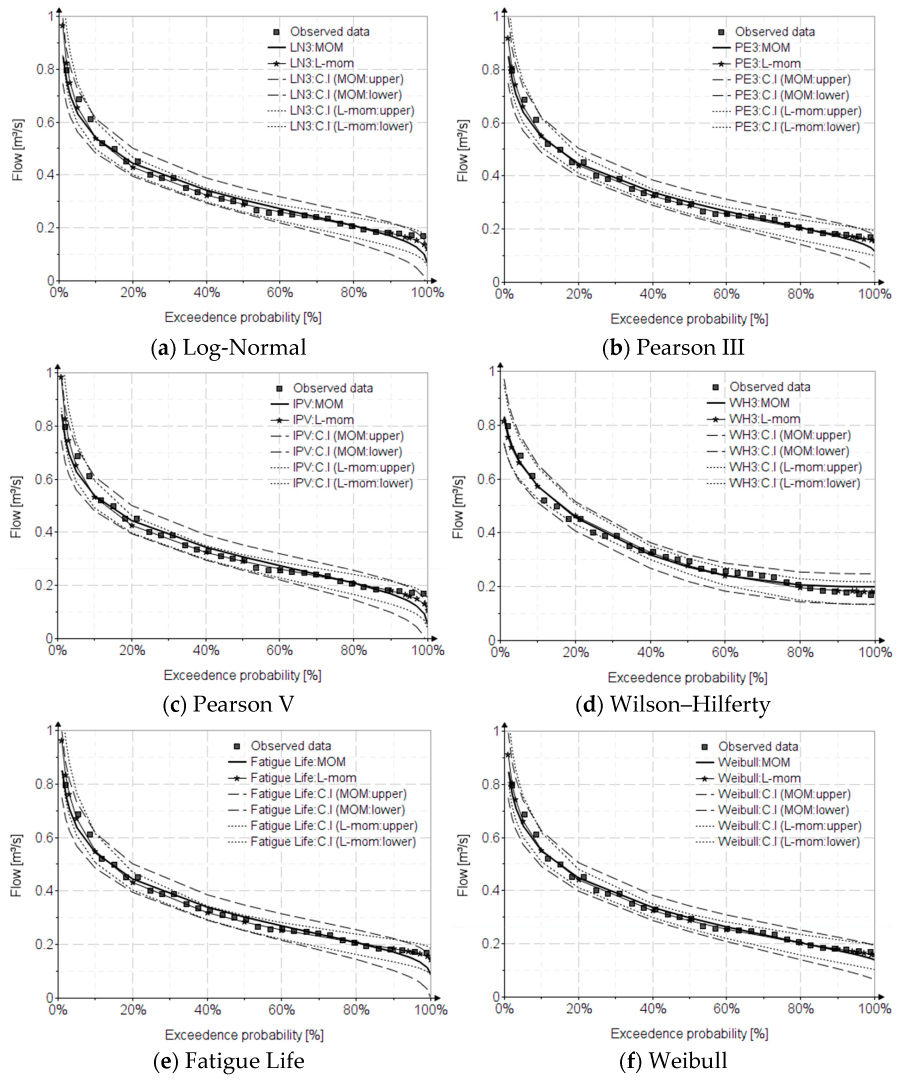
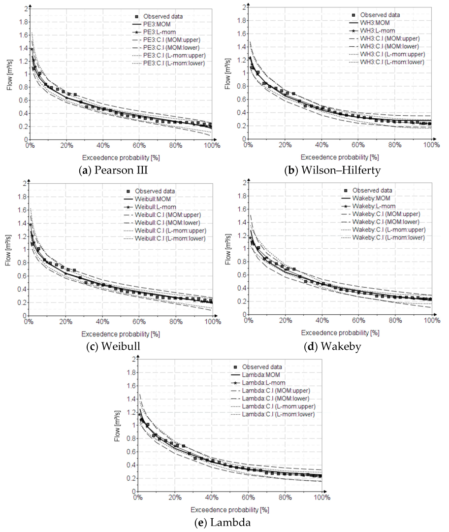
Figure 6, Figure 7 and Figure 8 show the frequency curves using the annual minimum flow (minimum 1-day flow), minimum 7-day flow, and minimum 30-day flow, respectively. For plotting positions, the Landwehr formula was used [18].
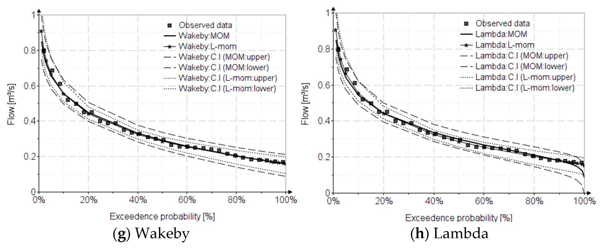
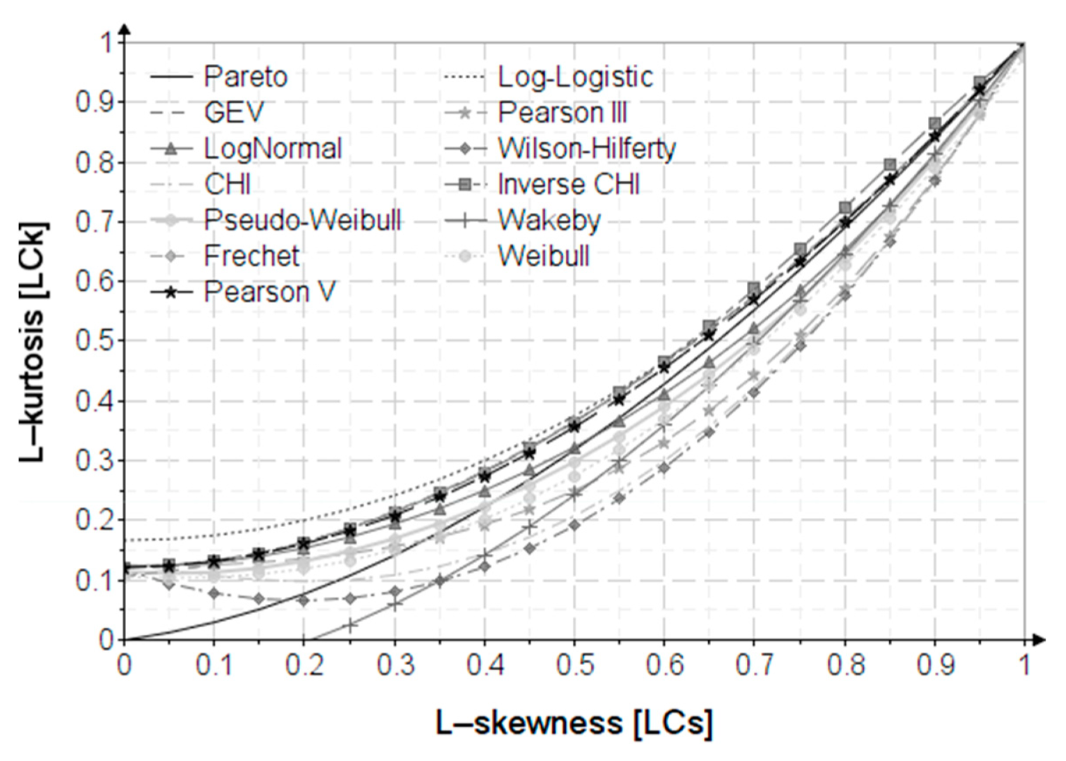
If the presented graphs are for three time series, the data are presented in the tables only for annual minimums, being specific to the run-of-river facilities. A frequency analysis was performed with distributions of three, four and five parameters for the two estimation methods, and the distributions that have a lower bound close to the minimum recorded value were selected. In general, it is considered that with a larger number of parameters, anything can be fit. In the case of parameter estimation with L-moments (the method recommended in this article, being much less influenced by the length of the observed data), it is necessary to estimate the first four linear moments, an aspect fulfilled properly only by distributions of at least four parameters. In the case of three-parameter distributions, they properly calibrate only L-skewness (L3/L2), and L-kurtosis (L4/L2) is the natural one of the distributions, not being able to calibrate according to the fourth order moment.
It should be mentioned, however, that not every distribution of at least four parameters gives good results; they must be used carefully, depending on the nature of extreme events (low flow or flood). In the analysis of extreme events, the most used are the Wakeby and lambda distributions, these having the advantage of the fact that the left hand is less influenced by the right hand, fulfilling the so-called ‘’separation effect’’ described by Matalas. Their advantage in the frequency analysis of low flows is represented by their asymptotic character in the field of high probabilities, with a lower bound close to the minimum value of the data sets.
The supplementary file graphically presents the results obtained for other four-parameter distributions (four-parameter kappa, four-parameter Kumaraswamy, four-parameter Burr, four-parameter Johnson SU). However, these cannot be applied for the analysis of the minimum extreme values, because for high probabilities of exceeding (right hand), they have a decreasing trend, being characterized by a small lower bound (even zero or negative); this is an unrealistic aspect for perennial rivers, generating unrealistic values in this field of probabilities.
From the case study, it is observed that among all the distributions analyzed, the ones that meet the conditions mentioned above are Wilson–Hilferty, Weibull, Wakeby and lambda. The Pearson III distribution was presented comparatively, because this is the parent distribution in Romania in the frequency analysis of extreme events. For the L-moments method, this gives good results.
Table 7 and Table 8 present the result values of quantiles for some of the most common exceedance probabilities for 1-day low flow analysis.
The resulting values of the estimated parameters are presented in Table 9, for both estimation methods, for 1-day low flow analysis.
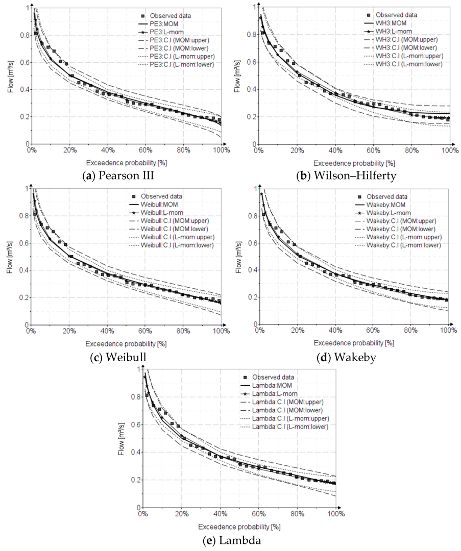
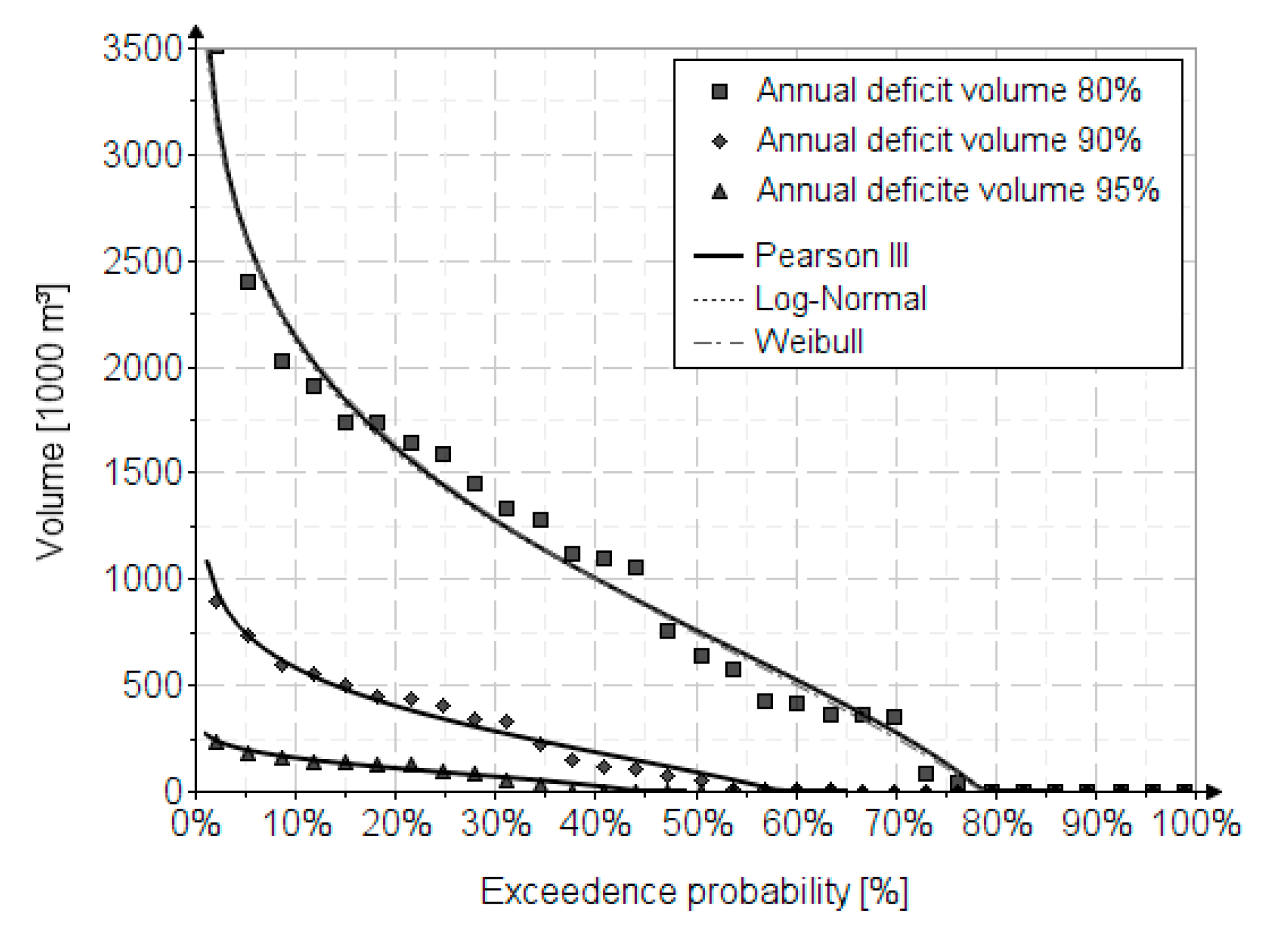
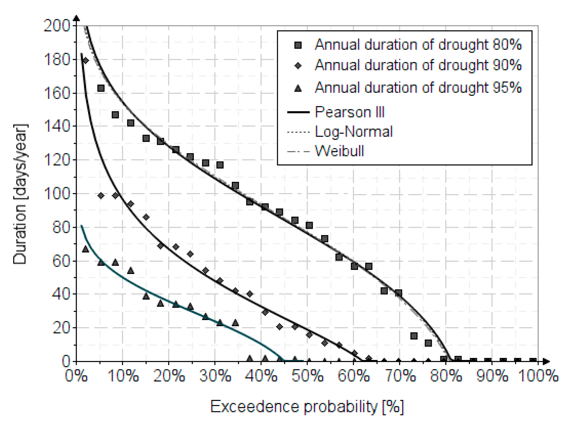
For the analysis of deficit volumes and durations of annual droughts, only three distributions of three parameters are presented. The calculations were made only for the estimation of parameters with L-moments, because MOM requires the choice of skewness, there being no criteria for this. The same considerations apply to the statistical analysis of drought durations. The distributions PE3 and W3 were chosen because they best estimate the data set, PE3 being also the parent distribution in Romania. The LN3 distribution is presented comparatively, as it is generally considered an alternative to PE3 [20].
Figure 9 shows the frequency curves used for the annual deficit volumes corresponding to the thresholds of 95%, 90% and 80%.
Table 10 presents the result values of quantiles for annual deficit volume.
Figure 10 shows the frequency curves used for the annual drought durations corresponding to the thresholds of 95%, 90% and 80%. The calculations were made only to estimate the parameters with L-moments.
Table 11 presents the result values of quantiles for annual drought duration.
The performance of the analyzed distribution was evaluated using the relative mean error (RME) and relative absolute error (RAE) criteria [40].
R M E = 1 n i = 1 n x i x p x i 2
R A E = 1 n i = 1 n x i x p x i
where n , x i , x p represent sample size, observed value, and estimated value for a given probability, respectively.
The distribution performance values are presented in Table 12, Table 13 and Table 14, only for the analysis of minimum annual flows (1-day), annual deficit volumes and annual drought durations.
We observed good performances for all the distributions used, for the probabilities defined on the range of observed values. For MOM estimation, the best approximation is the Wakeby distribution. For estimation with L-moments, a good approximation of L-skewness and L-kurtosis is observed for three distributions, Wakeby, lambda and Weibull.
In the case of the analysis for annual deficit volumes and annual drought durations, the performances are good for the distributions LN3 and PE3.

5. Conclusions

This article presents hydrological drought analysis using frequency analysis. Considering the complexity of this hydrological phenomenon, it is necessary to establish well-founded criteria regarding the analysis of minimum flows, deficit volumes and drought durations. Thus, this article presents the necessary criteria regarding the frequency analysis of minimum annual flows, the establishment of drought thresholds based on the duration curve of the average daily flows, as well as the deficit volumes and drought durations corresponding to the thresholds. A preferred analysis in hydrology is the use of average monthly flows, which often do not reflect the phenomenon of drought. In this article, the analysis with time series moving averages for 7 and 30 days is proposed [7]. The methodology provides the necessary mathematical support for frequency analysis of hydrological drought for the elaboration of a norm in Romania. Mathematical support in statistical analysis is useful, because the use of software (EasyFit, HEC-SSP, …) without knowledge of mathematical foundations often leads to superficial analyses with negative consequences in water management.
The case study consisted of hydrological drought analysis for the Prigor River. The frequency analysis was performed using eight probability distributions, their parameters being estimated with two of the most used parameter estimation methods in the analysis of extreme phenomena in hydrology. All the mathematical characteristics necessary for the application of the eight analyzed distributions, for the method of ordinary moments and the method of linear moments are presented.
For ease of application of these distributions, parameter approximations were made for MOM and L-moments.
For confidence interval calculation using Chow’s relation [37], Appendix A presents the frequency factor of distributions analyzed for both parameter estimation methods. A criterion for choosing distributions for L-moments analysis is the variance of τ 3 τ 4 . Figure A1 from Appendix B presents approximation relations of τ 4 with regards to τ 3 for a wide range of distributions used in hydrology.
A peculiarity in the analysis of the frequency of annual drought volumes and durations is the choice of thresholds. Many researchers avoid choosing minimum flow thresholds (Q90%,Q95%) that generate many zero values of volumes and durations, thus ignoring these values corresponding to these thresholds needed in water management. This impediment of threshold selection is solved by using conditional probabilities, which apply a correction to the cumulative function and implicitly to the inverse function.
All research was carried out within the Faculty of Hydrotechnics for elaboration of a norm regarding hydrological drought and for improving the legislation of ecological flow, based on mathematical methods for determining the water deficit.

Supplementary Materials

The following supporting information can be downloaded at: https://www.mdpi.com/article/10.3390/app13053055/s1. Figure S1: The probability distributions curves for minimum 1-day low flows, Table S1: The observed data from Prigor hydrometric station, Table S2: The statistical indicators of the observed values, Table S3: The annual volumes deficit, Table S4: The annual drought durations. References [25,26,29,41,42,43,44,45,46,47] are cited in the supplementary materials.

Author Contributions

Conceptualization, C.I. and C.G.A.; methodology, C.I. and C.G.A.; software, C.I. and C.G.A.; validation, C.I. and C.G.A.; formal analysis, C.I. and C.G.A.; investigation, C.I. and C.G.A.; resources, C.I. and C.G.A.; data curation, C.I. and C.G.A.; writing—original draft preparation, C.I. and C.G.A.; writing—review and editing, C.I. and C.G.A.; visualization, C.I. and C.G.A.; supervision, C.I. and C.G.A.; project administration, C.I. and C.G.A.; funding acquisition, C.I. and C.G.A. All authors have read and agreed to the published version of the manuscript.

Funding

This research received no external funding.

Institutional Review Board Statement

Not applicable.

Informed Consent Statement

Not applicable.

Data Availability Statement

Not applicable.

Conflicts of Interest

The authors declare no conflict of interest.

Abbreviations

MOMthe method of ordinary moments
L-momentsthe method of linear moments
μ expected value; arithmetic mean
σ standard deviation
C v coefficient of variation
C s coefficient of skewness; skewness
C k coefficient of kurtosis; kurtosis
L 1 , L 2 , L 3 linear moments
τ 2 , L C v coefficient of variation based on the L-moments method
τ 3 , L C s coefficient of skewness based on the L-moments method
τ 4 , L C k coefficient of kurtosis based on the L-moments method
ξ multiplication factor
Distr.Distributions
LN3three parameters log-normal distribution
FL3fatigue lifetime distribution
PE3Pearson III distribution
IPVthree-parameter Pearson V distribution
WH3three-parameter Wilson–Hilferty distribution
W3three-parameter Weibull distribution
WK5five-parameter Wakeby distribution
L5five-parameter lambda distribution
xi, Qobserved values
Qp%flow with exceedance probability of p%
Qmmultiannual average flow

Appendix A. The Frequency Factors for the Analyzed Distributions

Table A1 shows the expressions of the frequency factors for MOM and L-moments.
Table A1. Frequency factors.
Distr.Frequency factor, K p p
Quantile function (inverse function)
Method of ordinary moments (MOM)L-moments
x p = μ + σ K p p x p = L 1 + L 2 K p p
LN3 q l n o r m 1 p , α , β exp α + 1 2 β 2 exp β 2 1 exp β 2 + 2 α exp β q n o r m 1 p , 0 , 1 exp 0.5 β 2 e r f 0.5 β exp 0.5 β 2
PE3 q g a m m a 1 p , α α α π Γ α q g a m m a 1 p , α α Γ α + 0.5
IPV α 3 α 2 q g a m m a p , α 1 1 1 q g a m m a p , α 1 1 α 2 1 α 2 2 z
where
z = exp 4.083852739 11.442833473 ln α + 10.701793287 ln α 2 6.513639901 ln α 3 + 2.527142191 ln α 4 0.640389591 ln α 5 + 0.105546499 ln α 6 0.010903032 ln α 7 + 0.000641094 ln α 8 0.000016371 ln α 9
WH3 q g a m m a 1 p , α 1 3 Γ α + 1 3 Γ α Γ α + 2 3 Γ α Γ α + 1 3 2 Γ α 2 β L 2 q g a m m a 1 p , α 1 3 Γ α + 1 3 Γ α
W3 ln 1 p 1 α Γ 1 + 1 α Γ 1 + 2 α Γ 1 + 1 α 2 1 1 2 1 α ln 1 p 1 α 1 α Γ 1 α 1
WK5 α β 1 p β γ δ 1 p δ α β + 1 + γ δ 1 α 2 β + 1 2 2 β + 1 2 α γ β + 1 β + 1 δ δ 1 γ 2 δ 1 2 2 δ 1 α β 1 p β γ δ 1 p δ α β + 1 γ 1 δ α β + 1 β + 2 + γ 2 δ 1 δ
L5 p β α β + α λ β + 1 1 p δ α β + 1 λ δ + 1 λ δ 2 λ β + 1 + 4 α δ 2 + 6 α δ + 2 α β + 1 δ + 1 2 2 δ + 1 + α 2 β 2 β + 1 2 2 β + 1 2 α λ Γ β + 1 Γ δ + 1 Γ δ + β + 2 p β α β + α λ β + 1 1 p δ α β + 1 + λ δ + 1 α β β + 1 β + 2 λ δ δ + 1 δ + 2

Appendix B. The Formula for Sample L-Moments

For calculating the sample L-moments, the observed data x i must be in ascending order.
The sample L-moments are:
L 1 = b 0   first   L moment L 2 = 2 b 1 b 0   second   L moment   L 3 = 6 b 2 6 b 1 + b 0   third   L moment   L 4 = 20 b 3 30 b 2 + 12 b 1 b 0   fourth   L moment  
where b 0 , b 1 , b 2 , b 3 represent natural estimators, expressed as:
b 0 = 1 n i = 1 n x i
b 1 = 1 n i = 1 n x i i 1 n 1
b 2 = 1 n i = 1 n x i i 1 n 1 i 2 n 2
b 3 = 1 n i = 1 n x i i 1 n 1 i 2 n 2 i 3 n 3
where n is the length of data series.
Using the L-moments, the coefficients of variation, ( τ 2 ), skewness ( τ 3 ) and kurtosis ( τ 4 ) are defined as [14,15,16,17]:
  • τ 2 = L 2 L 1 —is the L-CV;
  • τ 3 = L 3 L 2 —is the L-Skewness;
  • τ 4 = L 4 L 2 —is the L-Kurtosis
In the next section, we present the variation of L-kurtosis, depending on the positive L-skewness, obtained with the L-moments method, for certain theoretical distributions often used in hydrology and in this article.
Figure A1. The variation diagram of L C s L C k .
Applsci 13 03055 g0a1
Pearson III:
τ 4 = 0.1217175 + 0.030285 τ 3 + 0.0266125 τ 3 2 + 0.8774691 τ 3 3 0.0564795 τ 3 4
Pearson V:
τ 4 = 0.1089545 0.1542626 τ 3 + 1.0657605 τ 3 2 0.3521005 τ 3 3 + 0.3269967 τ 3 4
Wilson–Hilferty:
τ 4 = 0.1177849 0.5367173 τ 3 + 1.4180786 τ 3 2 0.2084697 τ 3 3 + 0.2098975 τ 3 4
CHI:
τ 4 = 0.1274475 0.2174617 τ 3 0.0945508 τ 3 2 + 2.6572905 τ 3 3 2.369862 τ 3 4 + 0.9016064 τ 3 5
Inverse CHI:
τ 4 = 0.1215494 + 0.0260015 τ 3 + 0.6839989 τ 3 2 + 2.3432188 τ 3 3 7.9178585 τ 3 4 + 11.9165941 τ 3 5 8.06007 τ 3 6 + 1.8820702 τ 3 7
Pseudo-Weibull:
τ 4 = 0.1132189 0.1242052 τ 3 + 1.1329458 τ 3 2 0.4716246 τ 3 3 + 0.3449906 τ 3 4
Wakeby:
τ 4 = 0.07347 + 0.14443 τ 3 + 1.03879 τ 3 2 0.14602 τ 3 3 + 0.03357 τ 3 4
Pareto:
τ 4 = 0.0003668 + 0.2070484 τ 3 + 0.9264 τ 3 2 0.133564 τ 3 3
Generalized Extreme Value:
τ 4 = 0.1072214 + 0.1143838 τ 3 + 0.8341466 τ 3 2 0.0632425 τ 3 3 + 0.0074607 τ 3 4
Frechet:
τ 4 = 0.1069938 + 0.1155235 τ 3 + 0.8294258 τ 3 2 0.0528083 τ 3 3
Weibull:
τ 4 = 0.1057425 0.0753465 τ 3 + 0.6176919 τ 3 2 + 0.5065127 τ 3 3 0.1788008 τ 3 4
Log-Normal:
τ 4 = 0.1238145 0.032954 τ 3 + 0.9783895 τ 3 2 0.3929245 τ 3 3 + 0.3174611 τ 3 4
Log-Logistic:
τ 4 = 1 + 5 τ 3 2 6 0.16667 + 0.83333 τ 3 2
Paralogistic:
τ 4 = 0.1262814 + 0.0078207 τ 3 + 0.9179335 τ 3 2 0.0328508 τ 3 3 0.0190348 τ 3 4
InverseParalogistic:
τ 4 = 0.0577651 + 0.5568896 τ 3 0.2198157 τ 3 2 + 0.9069583 τ 3 3 0.3025029 τ 3 4

Appendix C. Distribution Equivalence Relations LCs-Cs

Table A2. Distribution equivalence relations.
DistributionSkewness
Generalized
Extreme
Value
C s = s i g n α 3 Γ 2 α + 1 Γ α + 1 Γ 3 α + 1 2 Γ α + 1 3 Γ 2 α + 1 Γ α + 1 2 3
α = 0.283759107 1.669931462 τ 3 1 + 0.441588375 τ 3 0.071007671 τ 3 2 + 0.015634368 τ 3 3
Log-Normal C s = 3 exp β 2 1 + exp β 2 1 3
if 0 < τ 3 1 3
β = 0.283759107 1.669931462 τ 3 1 + 0.441588375 τ 3 0.071007671 τ 3 2 + 0.015634368 τ 3 3
1 3 < τ 3 2 3
β = 5.3943247 10 2 + 2.6732827 τ 3 2.9211411 τ 3 2 + 7.3388138 τ 3 3 8.1997299 τ 3 4 + 4.3299046 τ 3 5
2 3 < τ 3 < 1
β = 0.81822527 + 7.818908 τ 3 4 8.1529453 τ 3 8 + 0.1554959 τ 3 12 1 + 2.5188862 τ 3 4 4.9742123 τ 3 8 + 1.592552 τ 3 12
Frechet C s = Γ 1 3 α + 2 Γ 1 1 α 3 3 Γ 1 2 α + Γ 1 1 α Γ 1 2 α Γ 1 1 α 2 3
α = 1 + 0.441588375 τ 3 0.071007671 τ 3 2 + 0.015634368 τ 3 3 0.283759107 + 1.669931462 τ 3
Weibull C s = Γ 1 + 3 α 3 Γ 1 + 2 α Γ 1 + 1 α + 2 Γ 1 + 1 α 3 Γ 1 + 2 α Γ 1 + 1 α 2 1.5
α = 3.528107902 6.294082546 τ 3 + 2.767652838 τ 3 2 1 + 4.599024923 τ 3 7.993601572 τ 3 2 + 2.423742593 τ 3 3
Log-Logistic C s = = Γ 1 + 3 α Γ 1 3 α + 2 Γ 1 + 1 α 3 Γ 1 1 α 3 3 Γ 1 + 2 α Γ 1 2 α Γ 1 + 1 α Γ 1 1 α Γ 1 + 2 α Γ 1 2 α Γ 1 + 1 α 2 Γ 1 1 α 2 1.5
α = 1 τ 3
Pareto C s = α α 2 α 1 2 α + 1 0.5 3 α + 1
α = 1 3 τ 3 τ 3 + 1
Pearson V C s = 4 α 3 0.5 α 4
α = exp 0.692740135 0.466055586 ln τ 3 + 0.460508385 ln τ 3 2 + 0.470172127 ln τ 3 3 + 0.938027763 ln τ 3 4 + 0.805363294 ln τ 3 5 + 0.359846034 ln τ 3 6 + 0.08945247 ln τ 3 7 + 0.011775528 ln τ 3 8 + 0.000641664 ln τ 3 9
Wilson–Hilferty C s = α 3 Γ α 2 Γ α + 2 3 Γ α + 1 3 + 2 Γ α 3 Γ α + 1 3 3 Γ α + 2 3 Γ α Γ α + 1 3 2 Γ α 2 Γ α + 2 3 Γ α + 1 3 2 Γ α
if 0 < τ 3 1 3
α = exp 4.16202506 3.261604018 ln τ 3 1.783702334 ln τ 3 2 0.770946644 ln τ 3 3 0.221698815 ln τ 3 4 0.041191426 ln τ 3 5 0.004665295 ln τ 3 6 0.000287712 ln τ 3 7 0.000007207 ln τ 3 8
1 3 < τ 3 2 3
α = exp 5.264027693 9.134993593 ln τ 3 15.845477811 ln τ 3 2 19.874003352 ln τ 3 3 15.495267042 ln τ 3 4 6.752325319 ln τ 3 5 1.255615645 ln τ 3 6
2 3 < τ 3 < 1
α = exp 7.712526023 93.06660109 ln τ 3 1.519099681 10 3 ln τ 3 2 1.602587644 10 3 ln τ 3 4 1.041173897 10 5 ln τ 3 4 4.152482998 10 5 ln τ 3 5 9.887282 10 5 ln τ 3 6 1.287749298 10 6 ln τ 3 7 7.050767642 10 5 ln τ 3 8
Pseudo-Weibull C s = 2 Γ 1 α 2 Γ 4 α + 8 Γ 2 α 3 9 Γ 1 α Γ 2 α Γ 3 α 4 3 4 Γ 1 α Γ 3 α Γ 2 α 2 1.5
α = 3.3784105 24.3298763 τ 3 + 1.3320721 10 2 τ 3 2 6.002157 10 2 τ 3 3 + 2.0552631 10 3 τ 3 4 5.037878 10 3 τ 3 5 + 8.5230901 10 3 τ 3 6 9.6216631 10 3 τ 3 7 + 6.8802849 10 3 τ 3 8 2.8078183 10 3 τ 3 9 + 4.9671387 10 2 τ 3 10
K3—
Generalized
Gumbel
C s = 0 1 ln α 1 1 p α ψ 1 α + 1 ln α γ e 3 0 1 l n α 1 1 p α 2 d p ψ 1 α + 1 + ln α + γ e 2 1.5 d p
if 0 < τ 3 1 / 3
α = 971.10886182 10 3 + 6.3606944 τ 3 6.35405524 τ 3 2 + 15.03572719 τ 3 3
1 / 3 < τ 3 < 1
α = 661.76303922 10 3 + 4.30832382 τ 3 1.09504916 τ 3 2 + 373.12384033 10 3 τ 3 3 1 999.98952576 10 3 τ 3
K3—Park C s = 2 Γ 2 α 3 α 3 α Γ 1 1 α 3 + Γ 1 α 2 Γ 4 α α 3 α Γ 1 3 α 3 Γ 1 α Γ 2 α Γ 3 α Γ 1 2 α Γ 1 1 α α 3 α Γ 1 α 3 Γ 3 α α 2 α Γ 1 2 α Γ 1 α Γ 2 α 2 α 2 α Γ 1 1 α 2 Γ 1 α 2 1.5
α = exp 0.000753505 0.983447042 ln τ 3 + 0.162877024 ln τ 3 2 + 0.247492727 ln τ 3 3 + 0.116264397 ln τ 3 4 + 0.029183504 ln τ 3 5 + 0.004031622 ln τ 3 6 + 0.000270699 ln τ 3 7 + 0.000005628 ln τ 3 8

Appendix D. The Central Moments of Wakeby and Lambda Distributions

The skewness and kurtosis coefficients for the Wakeby distribution are shown below:
C s = 6 · α · γ 2 · δ 2 δ · β + δ 1 β + 1 · β + 1 2 · δ · β + 1 δ · δ 1 2 · 2 · δ 1 + 6 · α 2 · γ · β 2 1 β · 1 + δ β + 1 2 · 2 · β + 1 · β + 1 δ · δ 1 · 2 · β + 1 δ 2 · γ 3 · 1 + δ δ 1 3 · 1 + δ · 6 · δ 5 2 · α 3 · β + 1 β + 1 3 · 1 + β · 5 + 6 · β α 4 β + 1 2 · 2 · β + 1 γ 2 δ 1 2 · 2 · δ 1 + 2 · α · λ β + 1 · δ 1 · δ β 1 1.5
C k = 3 · 4 · α · γ 4 · 3 + 2 · β + β 2 δ · 12 + β · 3 + β δ 2 11 + β + 2 · β 2 2 · δ 3 · 1 + 3 · β 4 · δ 4 1 + β · 1 + β 3 · δ · 1 + β 2 · δ · 1 + β δ · δ 1 3 · 1 + δ · 6 · δ 5 + α 4 · 2 · β 2 β + 3 β + 1 4 · 24 · β 3 + 26 · β 2 + 9 · β + 1 γ 4 · 3 + δ + 2 · δ 2 δ 1 4 · 4 · δ 1 · 1 + δ · 6 · δ 5 + 4 · α 3 · γ · 3 + 4 · β 4 + β 3 · 2 6 · δ + δ · δ 2 + β · 12 + δ · δ 3 + β 2 · 11 + δ · 2 · δ 1 1 + β 3 · 1 + β · 6 · β + 5 · 1 + β δ · 1 + 2 · β δ · 1 + 3 · β δ · δ 1 + 2 · α 2 · γ 2 · 9 β · 30 + β · 29 + 4 · β · 2 + β + β · δ · 71 + β · 43 + 2 · β · 7 + 4 · β δ 2 · 29 + β · 43 + 4 · 6 + 7 · β + 2 · δ 3 · 4 + 7 · β · 1 + 2 · β 4 · δ 4 · 1 + 2 · β + 30 · δ β + 1 2 · 2 · β + 1 · 1 + β 2 · δ · 1 + 2 · β 2 · δ · 1 + β δ · 1 + 2 · β δ · δ 1 2 · 2 · δ 1 γ 2 δ 1 2 · 2 · δ 1 α 4 β + 1 2 · 2 · β + 1 + 2 · α · λ β + 1 · δ 1 · δ β 1 2
The skewness and kurtosis coefficients for the lambda distribution are shown below:
C s = 1 σ 3 · λ 3 3 · δ + 1 + 3 · α · λ 2 · Γ β + 1 · Γ 2 · δ + 1 Γ β + 2 · δ + 2 3 · λ · μ 2 · δ + 1 + 3 · λ 2 · γ 2 · δ + 1 3 · α 2 · λ · Γ 2 · β + 1 · Γ δ + 1 Γ 2 · β + δ + 2 + 6 · α · λ · μ · Γ β + 1 · Γ δ + 1 Γ β + δ + 2 3 · λ · μ 2 δ + 1 + 6 · γ · λ · μ δ + 1 6 · α · λ · γ · Γ β + 1 · Γ δ + 1 Γ β + δ + 2 3 · γ 2 · λ δ + 1 + α 3 3 · β + 1 3 · α 2 · μ 2 · β + 1 + 3 · α 2 · γ 2 · β + 1 + 3 · α · μ 2 β + 1 6 · α · μ · γ β + 1 + 3 · α · γ 2 β + 1 μ 3 + 3 · γ · μ 2 3 · γ 2 · μ + γ 3
C k = 1 σ 4 · λ 4 4 · δ + 1 4 · α · λ 3 · Γ β + 1 · Γ 3 · δ + 1 Γ β + 3 · δ + 2 + 4 · λ 3 · μ 3 · δ + 1 4 · λ 3 · γ 3 · δ + 1 + 6 · α 2 · λ 2 · Γ 2 · β + 1 · Γ 2 · δ + 1 Γ 2 · β + 2 · δ + 2 12 · α · λ 3 · μ · Γ β + 1 · Γ 2 · δ + 1 Γ β + 2 · δ + 2 + 6 · λ 2 · μ 2 2 · δ + 1 + 4 · α 3 · γ 3 · β + 1 + 12 · α · λ 2 · γ · Γ β + 1 · Γ 2 · δ + 1 Γ β + 2 · δ + 2 12 · γ · λ 2 · μ 2 · δ + 1 + 6 · γ 2 · λ 2 2 · δ + 1 4 · α 3 · λ · Γ 3 · β + 1 · Γ δ + 1 Γ 3 · β + δ + 2 + 6 · α 2 · γ 2 2 · β + 1 4 · α · μ 3 β + 1 + 12 · α 2 · λ · μ · Γ 2 · β + 1 · Γ δ + 1 Γ 2 · β + δ + 2 + 4 · λ · μ 3 δ + 1 12 · α 2 · λ · γ · Γ 2 · β + 1 · Γ δ + 1 Γ 2 · β + δ + 2 + 12 · γ 3 · λ · μ δ + 1 12 · α · λ · μ 3 · Γ β + 1 · Γ δ + 1 Γ β + δ + 2 + 12 · α · γ · μ 2 β + 1 12 · α · γ 2 · μ β + 1 + α 4 4 · β + 1 4 · α 3 · μ 3 · β + 1 + 4 · α · γ 3 β + 1 + μ 3 4 · γ · μ 3 + 6 · γ 2 · μ 2 + 24 · α · λ · μ · γ · Γ β + 1 · Γ δ + 1 Γ β + δ + 2 12 · α · λ · γ 2 · Γ β + 1 · Γ δ + 1 Γ β + δ + 2 12 · γ · λ · μ 2 δ + 1 4 · γ 3 · λ δ + 1 + 6 · α 2 · μ 2 2 · β + 1 12 · α 2 · γ · μ 2 · β + 1 4 · γ 3 · μ + γ 4

Appendix E. The First Raw and Central Moments of IPV Distribution

To determine the raw moments of the Pearson V (IPV) distribution, the following substitutions in the expression for the probability density function are required:
f x = exp β x γ β Γ α 1 x γ β α
It is noted:
t = β x γ x = γ + β t d x = β t 2 d t
Thus, the first four raw moments are:
m 1 = γ x f x = γ x exp β x γ β Γ α 1 x γ β α d x = 1 Γ α 1 0 γ + β t t α 2 e t d t = γ Γ α 1 0 t α 2 e t d t + β Γ α 1 0 t α 3 e t d t = γ + β Γ α 1 Γ α 2
m 2 = γ x 2 f x = γ x exp β x γ β Γ α 1 x γ β α d x = 1 Γ α 1 0 γ + β t 2 t α 2 e t d t = γ 2 Γ α 1 0 t α 2 e t d t + 2 γ β Γ α 1 0 t α 3 e t d t + β 2 Γ α 1 0 t α 4 e t d t = γ 2 + 2 γ β Γ α 1 Γ α 2 + β 2 Γ α 1 Γ α 3
m 3 = γ x 3 · f x = γ x · exp β x γ β · Γ α 1 · x γ β α d x = 1 Γ α 1 · 0 γ + β t 3 · t α 2 · e t · d t = γ 3 Γ α 1 · 0 t α 2 · e t · d t + 3 · γ 2 · β Γ α 1 · 0 t α 3 · e t · d t + 3 · γ · β 2 Γ α 1 · 0 t α 4 · e t · d t + β 3 Γ α 1 · 0 t α 5 · e t · d t = γ 3 + 3 · γ 2 · β Γ α 1 · Γ α 2 + 3 · γ · β 2 Γ α 1 · Γ α 3 + β 3 Γ α 1 · Γ α 4
m 4 = γ x 4 · f x = γ x · exp β x γ β · Γ α 1 · x γ β α d x = 1 Γ α 1 · 0 γ + β t 4 · t α 2 · e t · d t = γ 4 Γ α 1 · 0 t α 2 · e t · d t + 4 · γ 3 · β Γ α 1 · 0 t α 3 · e t · d t + 6 · γ 2 · β 2 Γ α 1 · 0 t α 4 · e t · d t 4 · γ · β 3 Γ α 1 · 0 t α 5 · e t · d t + β 4 Γ α 1 · 0 t α 6 · e t · d t = γ 4 + 4 · γ 3 · β Γ α 1 · Γ α 2 + 6 · γ 2 · β 2 Γ α 1 · Γ α 3 + 4 · γ · β 3 Γ α 1 · Γ α 4 + β 4 Γ α 1 · Γ α 5
The first four centered moments have the following expressions:
m 1 = m 1 = μ = = γ + β α 1
m 2 = σ 2 = m 2 m 1 2 = β 2 α 3 α 2 2
m 3 = m 3 3 m 2 m 1 + 2 m 1 3 = 4 β 3 α 4 α 3 α 2 3
m 4 = m 4 4 m 3 m 1 + 6 m 2 m 1 2 3 m 1 4 = 3 β 4 α + 4 α 5 α 4 α 3 α 2 4
Skewness and kurtosis are determined with the following expressions:
γ 1 = C s = m 3 m 2 3 / 2 = 4 α 3 α 4
γ 2 = C k = m 4 m 2 2 = 3 α + 4 α 3 α 4 α 5

Appendix F. Built-in Function in Mathcad

  • Γ x —returns the value of the Euler gamma function of x;
  • Γ α , x —returns the value of the incomplete gamma function of x with parameter a;
  • d g a m m a x , s —returns the probability density for value x, for gamma distribution;
  • p g a m m a x , s —returns the cumulative probability distribution for value x, for gamma distribution;
  • q g a m m a p , s —returns the inverse cumulative probability distribution for probability p, for gamma distribution. This can also be found in other dedicated programs (the GAMMA.INV function in Excel).
  • q n o r m p , 0 , 1 —returns the inverse standard cumulative probability distribution for probability p, for Normal distribution,(NORM.INV function in Excel).
  • p l n o r m x , α , β —returns the cumulative probability distribution for value x, for log-normal distribution;
  • q l n o r m p , μ , σ —returns the inverse cumulative probability distribution for probability p, for log-normal distribution, (LOGNORM.INV function in Excel).
  • e r f x —returns the error function;

References

  1. Wilhite, D.A.; Glantz, M.H. Understanding the Drought Phenomenon: The Role of Definitions. Water Int. 1985, 10, 111–120. [Google Scholar] [CrossRef] [Green Version]
  2. Tallaksen, L.M.; van Lanen, H.A.J. (Eds.) Hydrological Drought—Processes and Estimation Methods for Streamflow and Groundwater, Developments in Water Sciences 48; Elsevier B.V.: Amsterdam, The Netherlands, 2004. [Google Scholar]
  3. Matalas, N.C. Probability Distribution of Low Flows. In Statistical Studies in Hydrology; Geological Survey; United States Covernment Printing Office: Washington, DC, USA, 1963. [Google Scholar]
  4. Dikici, M. Drought analysis with different indices for the Asi Basin (Turkey). Sci Rep 2020, 10, 20739. [Google Scholar] [CrossRef] [PubMed]
  5. Van Loon, A. Hydrological drought explained. Wiley Interdiscip. Rev. Water 2015, 2, 359–392. [Google Scholar] [CrossRef]
  6. Lang Delus, C. Les étiages: Définitions hydrologique, statistique et seuils réglementaires. Cybergeo Eur. J. Geogr. 2011. [Google Scholar] [CrossRef]
  7. World Meteorological Organization. (WMO-No.1029) 2008 Manual on Low-Flow Estimation and Prediction; Operational Hydrology Report no. 50; WHO: Geneva, Switzerland, 2008. [Google Scholar]
  8. Institute of Hydrology. (IH) 1992 Low Flow Estimation in the United Kingdom; Report no. 108; Institute of Hydrology: Lancaster, UK, 1992. [Google Scholar]
  9. UNESCO. Methods of Computation of Low Streamflow, Studies and Reports in Hydrology; UNESCO: Paris, France, 1982; ISBN 92-102013-7. [Google Scholar]
  10. Loganathan, G.V.; Kuo, C.Y.; McCormick, T.C. Frequency Analysis of Low Flow. Nord. Hydrol. 1985, 16, 105–128. [Google Scholar] [CrossRef] [Green Version]
  11. Bulletin 17B Guidelines for Determining Flood Flow Frequency; Hydrology Subcommittee; Interagency Advisory Committee on Water Data; U.S. Department of the Interior; U.S. Geological Survey; Office of Water Data Coordination: Reston, VA, USA, 1981.
  12. Bulletin 17C Guidelines for Determining Flood Flow Frequency; U.S. Department of the Interior; U.S. Geological Survey: Reston, VA, USA, 2017.
  13. H.G. 148/2020; The Method of Determining and Calculating the Ecological Flow. The Government of Romania: Bucharest, Romania, 2020.
  14. Stanca, S.C.; Dimache, A.N.; Ilinca, C.; Anghel, C.G. Methodology for determining hydromorphological indicators for rivers with hydropower uses. IOP Conf. Ser. Earth Environ. Sci. 2022, 1136, 012032. [Google Scholar] [CrossRef]
  15. Hosking, J.R.M. L-moments: Analysis and Estimation of Distributions using Linear, Combinations of Order Statistics. J. R. Statist. Soc. 1990, 52, 105–124.C. [Google Scholar] [CrossRef]
  16. Hosking, J.R.M.; Wallis, J.R. Regional Frequency Analysis, An Approach Based on L-Moments; Cambridge University Press: Cambridge, UK, 1997; ISBN 13 978-0-521-43045-6. [Google Scholar]
  17. World Meteorological Organization. (WMO-No.100) 2018 Guide to Climatological Practices; WMO: Geneva, Switzerland, 2018. [Google Scholar]
  18. Rao, A.R.; Hamed, K.H. Flood Frequency Analysis; CRC Press LLC: Boca Raton, FL, USA, 2000. [Google Scholar]
  19. Ilinca, C.; Anghel, C.G. Flood-Frequency Analysis for Dams in Romania. Water 2022, 14, 2884. [Google Scholar] [CrossRef]
  20. Anghel, C.G.; Ilinca, C. Parameter Estimation for Some Probability Distributions Used in Hydrology. Appl. Sci. 2022, 12, 12588. [Google Scholar] [CrossRef]
  21. Singh, V.P. Entropy-Based Parameter Estimation in Hydrology; Springer Science + Business Media: Dordrecht, The Netherlands, 1998; ISBN1 978-90-481-5089-2. ISBN2 978-94-017-1431-0. [Google Scholar] [CrossRef]
  22. Constantinescu, M.; Golstein, M.; Haram, V.; Solomon, S. Hydrology; Technical Publishing House: Bucharest, Romania, 1956. [Google Scholar]
  23. Mandru, R.; Ioanitoaia, H. Ameliorative Hydrology; Agro-Silvica Publishing House: Bucharest, Romania, 1962. [Google Scholar]
  24. Bejenaru, G.; Castravet, T.; Dilan, V. Hydrological Calculations; Print Caro Publishing House: Chisinau, Moldova, 2020. [Google Scholar]
  25. Papukdee, N.; Park, J.-S.; Busababodhin, P. Penalized likelihood approach for the four-parameter kappa distribution. J. Appl. Stat. 2021, 49, 1559–1573. [Google Scholar] [CrossRef]
  26. Shin, Y.; Park, J.-S. Modeling climate extremes using the four-parameter kappa distribution for r-largest order statistics. Weather. Clim. Extrem. 2023, 39, 100533. [Google Scholar] [CrossRef]
  27. Çitakoğlu, H.; Demir, V.; Haktanir, T. L−Momentler yöntemiyle karadeniz’e dökülen akarsulara ait yillik anlik maksimum akim değerlerinin bölgesel frekans analizi. Ömer Halisdemir. Üniversitesi. Mühendislik Bilim. Derg. 2017, 6, 571–580. [Google Scholar] [CrossRef] [Green Version]
  28. Teodorescu, I.; Filotti, A.; Chiriac, V.; Ceausescu, V.; Florescu, A. Water Management; Ceres Publishing House: Bucharest, Romania, 1973. [Google Scholar]
  29. Crooks, G.E. Field Guide to Continuous Probability Distributions; Berkeley Institute for Theoretical Science: Berkeley, CA, USA, 2019. [Google Scholar]
  30. STAS 4068/1962; Maximum Water Discharges and Volumes, Determination of Maximum Water Discharges and Volumes of Watercourses. The Romanian Standardization Institute: Bucharest, Romania, 1962.
  31. Diaconu, C.; Serban, P. Syntheses and Hydrological Regionalization; Technical Publishing House: Bucharest, Romania, 1994. [Google Scholar]
  32. Abramowitz, M.; Stegun, I.A. Handbook of Mathematical Functions with Formulas, Graphs, and Mathematical Tables. Am. J. Phys. 1988, 56, 958. [Google Scholar] [CrossRef] [Green Version]
  33. Li, H.; Wen, D.; Lu, Z.; Wang, Y.; Deng, F. Identifying the Probability Distribution of Fatigue Life Using the Maximum Entropy Principle. Entropy 2016, 18, 111. [Google Scholar] [CrossRef] [Green Version]
  34. Alghamdi, S.M.; Bantan, R.A.R.; Hassan, A.S.; Nagy, H.F.; Elbatal, I.; Elgarhy, M. Improved EDF-Based Tests for Weibull Distribution Using Ranked Set Sampling. Mathematics 2022, 10, 4700. [Google Scholar] [CrossRef]
  35. Houghton, J.C. Birth of a parent: The Wakeby distribution for modeling flood flows. Water Resour. Res. 1978, 14, 1105–1109. [Google Scholar] [CrossRef] [Green Version]
  36. Greenwood, J.A.; Landwehr, J.M.; Matalas, N.C.; Wallis, J.R. Probability Weighted Moments: Definition and Relation to Parameters of Several Distributions Expressable in Inverse Form. Water Resour. Res. 1979, 15, 1049–1054. [Google Scholar] [CrossRef] [Green Version]
  37. Chow, V.T.; Maidment, D.R.; Mays, L.W. Applied Hydrology; MCGraw-Hill, Inc.: New York, NY, USA, 1988; ISBN 007-010810-2. [Google Scholar]
  38. The Romanian Water Classification Atlas, Part I—Morpho-Hydrographic Data on the Surface Hydrographic Network; Ministry of the Environment: Bucharest, Romania, 1992.
  39. STAS 1343/0-89; Determining Water Supply Quantities. The Romanian Standardization Institute: Bucharest, Romania, 1989.
  40. Singh, V.P.; Singh, K. Parameter Estimation for Log-Pearson Type III Distribution by Pome. Hydraul. Eng. 1988, 114, 112–122. Available online: https://hdl.handle.net/1969.1/164673 (accessed on 3 March 2012). [CrossRef]
  41. D’Adderio, L.; Cugerone, K.; Porcu, F.; de michele, C.; Tokay, A. Capabilities of the Johnson SB distribution in estimating rain variables. Adv. Water Resour. 2016, 97, 241–250. [Google Scholar] [CrossRef]
  42. Hosking, J.R.M. The four-parameter kappa distribution. IBM J. Res. Dev. 1994, 38, 251–258. [Google Scholar] [CrossRef]
  43. Hao, Z.; Singh, V. Entropy-Based Parameter Estimation for Extended Three-Parameter Burr III Distribution for Low-Flow Frequency Analysis. Trans. ASABE 2009, 52, 1193–1202. [Google Scholar] [CrossRef]
  44. Bhatti, F.; Ali, A.; Hamedani, G.; Ahmad, M. On Generalized Log Burr Xii Distribution. Pak. J. Stat. Oper. Res. 2018, 14, 615. [Google Scholar] [CrossRef]
  45. Carrasco, J.; Ferrari, S.; Cordeiro, G. A New Generalized Kumaraswamy Distribution. arXiv 2010, arXiv:1004.0911. [Google Scholar]
  46. Dey, S.; Mazucheli, J.; Nadarajah, S. Kumaraswamy Distribution: Different Methods of Estimation. J. Comput. Appl. Math. 2017, 37. [Google Scholar] [CrossRef]
  47. Tian, W.; Pang, L.; Tian, C.; Ning, W. Change Point Analysis for Kumaraswamy Distribution. Mathematics 2023, 11, 553. [Google Scholar] [CrossRef]
Figure 1. Duration curves for Prigor river.
Applsci 13 03055 g001
Figure 2. Determining drought volumes and durations for the Q80% threshold.
Applsci 13 03055 g002
Figure 3. Methodological approach.
Applsci 13 03055 g003
Figure 4. The Prigor River location—Prigor hydrometric station.
Applsci 13 03055 g004
Figure 5. Water deficit graph for the Prigor River for the WMO reference period.
Applsci 13 03055 g005
Figure 6. The probability distribution curves for minimum 1-day low flows.
Applsci 13 03055 g006aApplsci 13 03055 g006b
Figure 7. The probability distribution curves for minimum 7-day low flows.
Applsci 13 03055 g007
Figure 8. The probability distribution curves for minimum 30-day low flows.
Applsci 13 03055 g008
Figure 9. The probability distribution curves for annual deficit volume.
Applsci 13 03055 g009
Figure 10. The probability distribution curves for annual deficit volume.
Applsci 13 03055 g010
Table 1. Novelty elements.
A. DistributionNew Elements
Fatigue Lifetimeinverse function; approximate relation for the shape parameter estimation with the L-moments method
Wakebythe first four central moments for parameter estimation with the method of ordinary moments
Lambdathe first four central moments for parameter estimation with the method of ordinary moments
B. Frequency factorsthe frequency factors for expressing the inverse functions of the distributions with MOM and L-moments
The international materials do not contain references regarding the expression of the inverse function of statistical distributions with the L-moments method.
C. Distribution equivalence relations LCs-CsThe equivalence relations between the two methods are presented for an easy transition from MOM to L-moments.
D. τ 4 τ 3 relationsThe variation is presented for a number of 15 distributions. In the case of the existing relations, presented in other materials, for PE3, GEV, W3, LN3, the relations have been improved, and in the case of the Pearson V, WH3, Chi, Inverse Chi, Pseudo-Weibull, Fréchet, Paralogistic, Inverse Paralogistic distributions, the relations are new.
E. Duration curveApproximation of duration curves with polynomials with logarithmic argument
Table 2. The morphometric characteristics.
Length
[km]
Average
Stream Slope [‰]
Sinuosity
Coefficient [-]
Average
Altitude, [m]
Drainage
Area, [km2]
33221.83713153
Table 3. The observed data from Prigor hydrometric station.
Minimum 1-Day Low Flows
19901991199219931994199519961997199819992000
Flow[m3/s]0.2570.3350.2500.2490.1700.3100.2350.7960.4000.5000.258
20012002200320042005200620072008200920102011
Flow[m3/s]0.2680.3300.2940.3000.4500.6100.4500.2410.3500.5200.193
201220132014201520162017201820192020
Flow[m3/s]0.2160.1730.6870.1800.3880.2070.1820.1850.390
Table 4. The statistical indicators of the data series.
Low FlowsStatistical Indicators
μ σ C v C s C k L 1 L 2 L 3 L 4 τ 2 τ 3 τ 4
[m3/s][m3/s][-][-][-][m3/s][m3/s][m3/s][m3/s][-][-][-]
minimum 1-day0.3350.1570.4691.3594.5930.3350.0840.0260.0130.2510.3070.152
Where μ , σ , C v , C s , C k , L 1 , L 2 , L 3 , L 4 , τ 2 , τ 3 , τ 4 represent the mean, the standard deviation, the coefficient of variation, the skewness, the kurtosis, the four L-moments, the L-coefficient of variation, the L-skewness, and the L-kurtosis, respectively P.
Table 5. The annual volume deficit.
95% Threshold
19901991199219931994199519961997199819992000
W[1000 m3]280.049.60.4164.40.04.40.00.00.01.4
20012002200320042005200620072008200920102011
W[1000 m3]1.50.00.00.00.00.00.0131.70.00.0100.8
201220132014201520162017201820192020
W[1000 m3]82133.80.0179.70.0233141.1122.80.0
W[1000 m3]3511.81907.70.01276.2359.12402.31642.21338.4366.9
Table 6. The annual drought durations.
95% Threshold
19901991199219931994199519961997199819992000
D[days/year]230.0232.0540.01.00.00.00.02.0
20012002200320042005200620072008200920102011
D[days/year]1.00.00.00.00.00.00.0590.00.034
201220132014201520162017201820192020
D[days/year]59390.0350.06733270.0
Table 7. Quantile results with MOM.
P
[%]
Probability Distributions
LN3PE3IPVWH3FL3W3WK5L5
[m3/s]
500.3040.2990.3060.2720.3010.2960.2900.297
700.2400.2350.2410.2180.2380.2320.2280.237
900.1690.1720.1670.1990.1710.1740.1790.179
950.1420.1520.1380.1980.1470.1580.1690.159
970.1260.1420.1210.1980.1340.1510.1650.147
Table 8. Quantile results with L-moments.
P
[%]
Probability Distributions
LN3PE3IPVWH3FL3W3WK5L5
[m3/s]
500.2900.2870.2910.2790.2840.2870.2870.286
700.2340.2280.2360.2150.2300.2270.2270.227
900.1800.1800.1800.1860.1850.1800.1800.181
950.1630.1690.1600.1840.1720.1690.1700.170
970.1530.1640.1490.1830.1650.1650.1660.166
Table 9. The estimated values of the parameters.
ParameterDistributions
LN3PE3IPVWH3FL3W3WK5L5LN3PE3IPVWH3FL3W3WK5L5
MOML-moments
α −1.1212.02413.00.1290.4821.2642.7 × 10−4−3.487−1.641.1766.1420.1530.8011.070.027−4.1
β 0.4210.1105.4510.5193.4900.2123.9840.0450.6440.1521.2960.5076.3120.1813.9840.043
γ −0.0220.112−0.1610.19814.770.1380.1992.3380.0950.1550.0220.183125.60.1580.1772.77
λ -------−1.353-------−1.49
δ ------−0.1300.013------−0.0410.001
ξ ------0.159-------0.160-
Table 10. Quantile results for annual deficit volume.
DistributionsProbability [%]
5102030405060708090
95% threshold—[1000 m3]
LN3193.01154.51106.0166.7123.5100000
PE3196.16154.69106.0666.6323.3500000
W3194.24156.61107.0565.8321.0100000
Table 11. Quantile results for annual drought duration.
DistributionsProbability [%]
5102030405060708090
95% threshold—[days/year]
LN360.8449.8135.5323.6210.1400000
PE360.8549.8335.5423.6110.1300000
W361.1150.3335.8323.429.4500000
Table 12. Distribution performance values for minimum annual flows.
DistributionMethods of Parameter EstimationObserved
Data
MOML-moments
RMERAERMERAE τ 3 τ 4 τ 3 τ 4
[-][-][-][-]
LN30.01690.05770.00870.03420.3070.1970.3070.152
PE30.01140.04310.00570.02570.159
IPV0.01870.06320.01020.03920.212
WH30.01240.05730.00960.04440.083
FL30.01410.04950.00660.03060.186
W30.00870.03670.00560.02540.155
WK50.00580.02730.00550.02530.152
L50.01100.04010.00560.02560.152
Table 13. Distribution performance values for annual deficit volumes.
DistributionMethods of Parameter Estimation
L-moments
RMERAE
95% threshold
LN30.21180.7498
PE30.21190.7498
W30.21210.7497
Table 14. Distribution performance values for annual drought durations.
DistributionMethods of Parameter Estimation
L-moments
RMERAE
95% threshold
LN30.20870.7343
PE30.20870.7343
W30.20930.7357
Disclaimer/Publisher’s Note: The statements, opinions and data contained in all publications are solely those of the individual author(s) and contributor(s) and not of MDPI and/or the editor(s). MDPI and/or the editor(s) disclaim responsibility for any injury to people or property resulting from any ideas, methods, instructions or products referred to in the content.

