Signal Control Study of Oversaturated Heterogeneous Traffic Flow Based on a Variable Virtual Waiting Zone in Dedicated CAV Lanes

Abstract

To meet the demand for cooperative signal control at oversaturated heterogeneous traffic flow intersections containing CAVs and HVs, cooperative control including dedicated CAV lanes has been explored to improve intersection safety capacity and reduce vehicle delays while avoiding uncertain HV driving behaviour. However, this approach does not fully exploit CAV network connectivity advantages and intersection spatial and temporal resources. Here, an oversaturated heterogeneous traffic flow signal control model based on a variable virtual waiting zone with a dedicated CAV lane is proposed. Within the model, CAVs going straight or left share a dedicated CAV lane, a CAV variable virtual waiting zone is within the intersection ahead of the dedicated CAV lane, and CAVs and HVs share the straight-through lane. The model framework has three layers. The upper layer optimizes the barrier time using a rolling time domain scheme. The middle layer optimizes the phase duration and variable virtual waiting zone switching time based on the fixed phase sequence, returning the vehicle delay to the upper optimization model. The lower layer performs CAV grouping and trajectory planning in the dedicated CAV lane based on signal timing and variable virtual waiting zone duration, returning the CAV delays to the middle level.

1. Introduction

Networked signals from advanced communication devices and other detection devices can sense intersection traffic demand and make intelligent control decisions [1,2,3]. Over time, the rapid development of vehicle-to-everything (V2X) and connected and automated vehicle (CAV) technologies will provide more real-time information about vehicles at signalized intersections and optimize vehicle trajectories [4]. A common belief among policy makers and scholars is that heterogeneous traffic flows with HV and CAV coexistence will be prevalent in the next 20–30 years [5,6,7]. The construction of China’s urban roads and increasing car ownership have made peak traffic flows at urban road intersections saturated or oversaturated [8,9,10]. Collaborative control of heterogeneous traffic flows based on dedicated CAV lanes has been explored to improve intersection capacity and reduce vehicle delays while avoiding uncertainty in HV driving behaviour [11,12,13,14,15]. Based on these advanced technologies and realistic situations, we need to study a new oversaturated heterogeneous traffic flow signal control model with a variable virtual waiting zone based on dedicated CAV lanes to utilize the advantages of CAV network linkages and exploit the spatiotemporal resources of intersections. This new signal control model consists of signal cycle control, dedicated lane variable virtual waiting zone time division, and vehicle trajectory control.

However, the challenges of the new signal control model include the following three aspects. First, the signal control period and phase duration are directly related to intersection traffic efficiency and vehicle delay duration, and reasonable regulation of the signal control period needs to fully consider the minimum vehicle delay at the entrance. Second, to fully exploit the space-time resources inside an intersection, the length and holding time of the variable virtual waiting zone need to be set reasonably. Third, the trajectory planning and grouping of CAVs in dedicated lanes also becomes complicated under oversaturated heterogeneous traffic demand.

In this paper, our objectives are to solve the above problems. An oversaturated heterogeneous traffic flow signal cooperative control model based on a variable virtual waiting zone for dedicated CAV lanes is proposed. The contributions of this study include signal cycle duration optimization, variable virtual waiting zone maintenance time optimization, and CAV trajectory optimization.

(1) An oversaturated heterogeneous traffic-flow cooperative signal-control model based on a variable virtual waiting zone in a dedicated CAV lane is proposed for the first time. The three-level structure of this model has coupling constraints and nested correlations. The variable virtual waiting zone can provide terminal constraints for a CAV to optimize its trajectory within the dedicated lane. The period and phase duration of the signal are based on the delay of the heterogeneous traffic flow, and the determination of the delay depends on the maintenance time of the variable virtual waiting zone and the trajectory planning of the CAV. Therefore, these three components are considered in this paper in an interrelated and comprehensive manner.

(2) Different from existing dedicated CAV lanes, to improve intersection capacity and reduce vehicle delays strategy we propose a variable virtual waiting zone concept based on dedicated CAV lanes combined with signal phasing. The variable virtual waiting zone fully exploits the spatial and temporal value of intersections and organically integrates the signal and CAV network characteristics to provide redundant space for CAV trajectory planning.

The remainder of this essay is structured as follows. Section 2 examines related research. The issue is discussed in Section 3 together with introduction of the variable virtual waiting zone. Section 4 presents the variable virtual waiting zone oversaturated heterogeneous traffic flow traffic signal and vehicle trajectory control model based on dedicated CAV lanes. Section 5 simulates and analyses the relevant results to reach conclusions. The work is concluded in Section 6, which also provides suggestions for additional research.

2. Related Work

2.1. Traffic Signal Control

Signal control based on vehicle arrival data can improve traffic sustainability and traffic efficiency. For signal optimization problems based on CAV arrival data, including green light duration optimization and phase sequence adjustment [16,17,18,19,20,21,22], the input for signal optimization is usually vehicle arrival information. In order to optimize the signal timing and phase sequence in a connected car environment, Feng et al. [17] suggested a real-time adaptive phase adjustment technique based on vehicle speed and spatial data. The experimental results show that the proposed algorithm has the ability to significantly reduce traffic delay. Shaghaghi et al. [18] included additional traffic data to use vehicle trajectory data as input for signal optimization, such as intersection waiting duration and traffic demand, including breakdowns and jumps. The signal optimization model is typically built using the National Electrical Manufacturers Association (NEMA) industry standard traffic signal structure optimizer [17,22]. In addition, Macroscopic Fundamental Diagram (MFD)-based traffic performance metrics is also used as input information for signal optimization [23]. To identify junction signal timing techniques, including signal cycle length and red and green light durations, Jiang et al. [22] used a phase-controlled optimization model. The experimental results showed that the suggested optimization strategy could increase traffic efficiency while maintaining high standards. Other variables such as fuel consumption and driving comfort are frequently seen as goals of optimization problems in addition to vehicle delay. It has been demonstrated that approaches such as dynamic programming and mixed-integer linear programming can be utilized to solve these issues [24]. However, these studies only consider the optimization of traffic signals, ignoring the optimization of vehicle trajectories, especially the random model problems [25,26,27] caused by the random arrival of vehicles, which may affect the performance of relevant strategies.

2.2. Optimal Control of Waiting Zones

Road signal intersection capacity can be effectively increased by intersection waiting zones during peak hours [28,29]. Intersection waiting zones usually include left-turn waiting zones and straight-through waiting zones [30,31,32]. Geometric layout, signal phasing, and suggested optimal traffic conditions are the current focus of studies on optimal waiting zone control. Yang et al. [31] systematically analysed the effects of waiting zones on vehicle average delay and vehicle fuel consumption under different green time ratios and different traffic demands through numerical simulations. Intersection safety and sustainability are often considered key indicators for evaluating the level of optimal control of intersection waiting zones [33,34]. When comparing scenarios of crossings with and without waiting zones, Jiang et al. [33] employed traffic conflict approaches and an ordered probability model to identify key variables that affect the severity of conflicts in waiting zones. The results of the study indicate that for manually driven vehicles, the use of a waiting zone increases intersection conflicts, bringing about secondary stops or repeated acceleration of vehicles inside the waiting zone. Unreasonable speed performance is also a negative contributor to fuel consumption and emissions [35]. The net-linked characteristics of CAVs have natural advantages to enhance the safety of intersection waiting zones and help in CAV trajectory planning in waiting zones [36]. Unfortunately, little research has been performed on waiting zones based on the net-linked characteristics of CAVs, including the waiting zone length, direction, and vehicle speed.

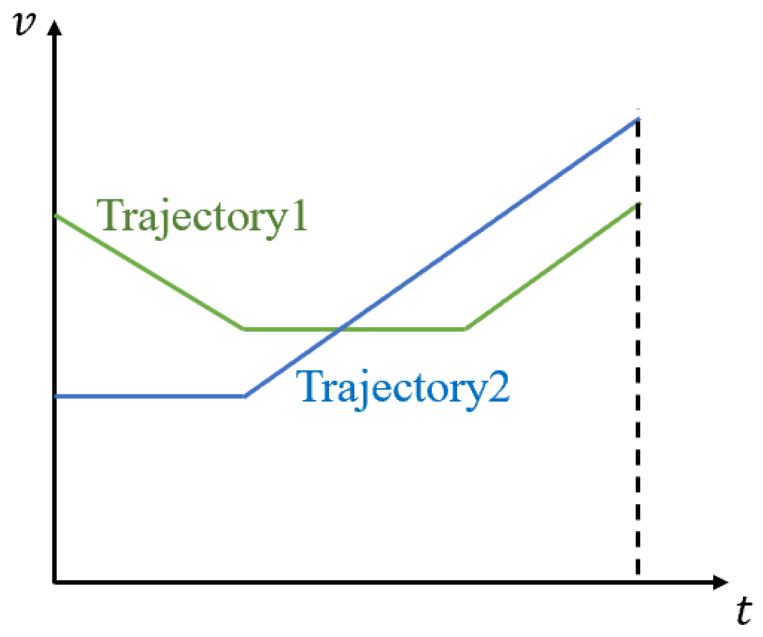
2.3. CAV Trajectory Optimization for Saturated Heterogeneous Traffic Flows

Optimal CAV trajectory control at intersections based on dedicated CAV lanes can ensure traffic safety and improve the operational efficiency of saturated heterogeneous traffic flows [12,14,37]. CAV trajectory planning at intersections based on dedicated CAV lanes includes planning to reduce energy consumption and shorten traffic delay [38,39,40,41,42,43,44]. Zhao et al. [42] suggested a model predictive control method to achieve mixed CAV platoons and HV platoons to minimize fuel consumption through signalized intersections. Malikopoulos et al. [43] created an analytical model for controlling CAV trajectory and solved the model from the standpoint of severe safety constraints. Additionally, various cutting-edge control techniques for vehicles, such as numerical computation, are suggested. Ma [44] proposed a decentralized planning approach for CAV trajectories. Based on a two-layer model, Ma optimized the longitudinal and lateral trajectories of individual CAVs. In the objective function, Ma considered vehicle delays, fuel consumption, and lane-change cost. It employed a parallel Monte Carlo tree-search technique and a lane-change strategy tree. Some numerical solution algorithms, including gradient-based methods [41] and metaheuristic algorithms [45], also provide new perspectives for solving CAV trajectory optimization problems. Unfortunately, CAV trajectory optimization near intersections often needs to be considered in conjunction with signal phasing because of vehicle motion continuity. Ma [11] proposed a dedicated CAV lane segregated intersection control model based on a shared phase dedicated lane (SPDL) for a mixed traffic environment, which is based on a dedicated CAV lane and unifies and optimizes CAV trajectory planning and signalized phase control to reduce the delay of heterogeneous traffic flow. However, the above problems in CAV trajectory planning for saturated heterogeneous traffic flow ignore the value of the waiting zone, and no method has been developed for CAV trajectory planning regarding signal phasing and having a waiting zone, which may play an important role in the above strategies.

3. Description of Related Problems

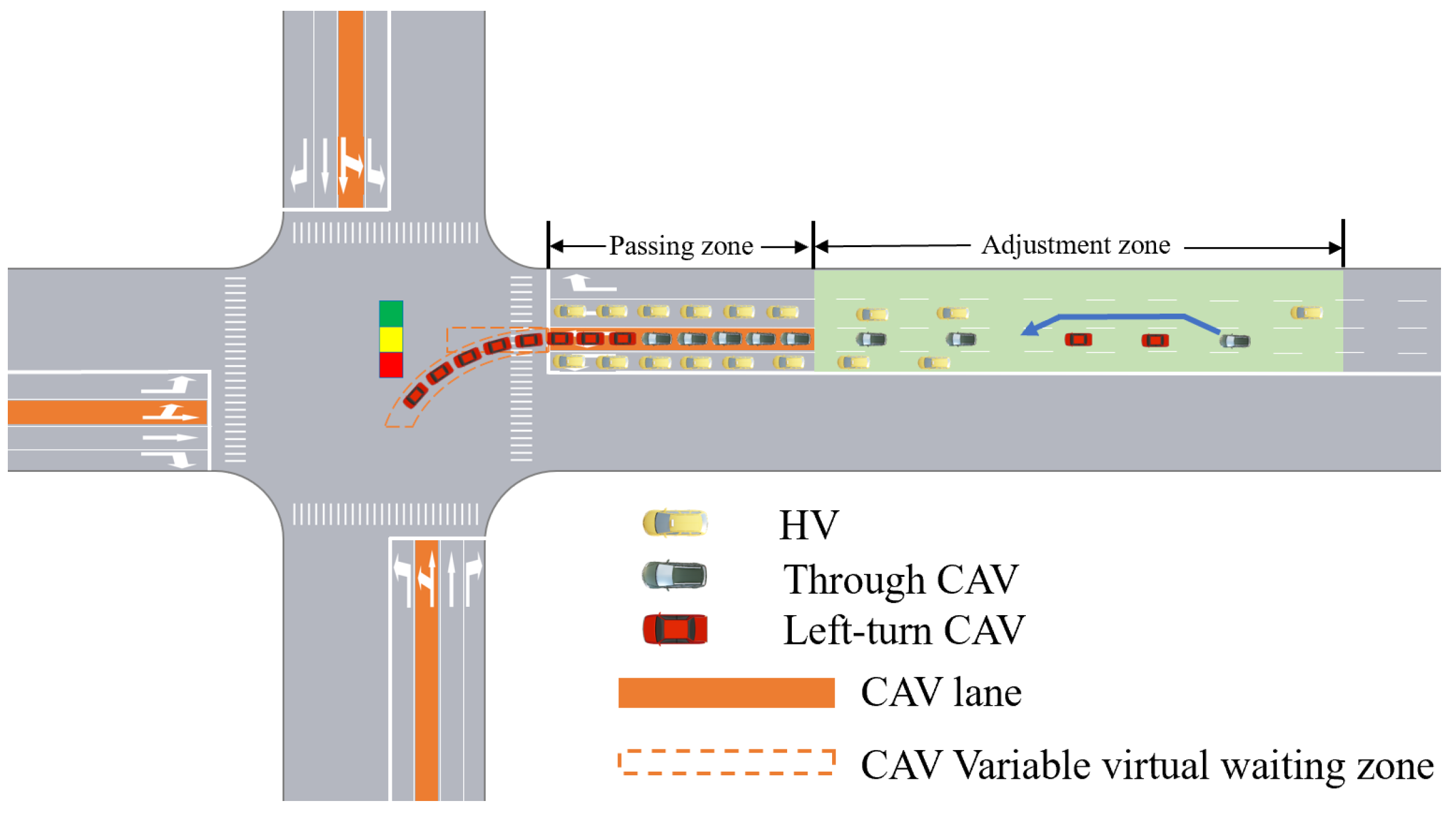
3.1. Traffic Signal Control

Figure 1 shows the layout of a common crossover with isolated intersections. Each arm has vehicles that travel in three different directions: left, straight ahead, and right. There is a dedicated CAV lane on each arm for straight-ahead and left-turn CAVs. Right-turn traffic signals are not used to govern CAVs and HVs as they operate in the right-turn lane. There is a passing zone and an adjustment zone on each arm close to the intersection. A CAV variable virtual waiting zone is set in the intersection in front of the passing zone, and the precise physical location of the signal intersection determines the size of the virtual waiting zone. the direction of the virtual waiting zone is determined by the control system. The CAVs are adjusted by the adjustment zone to form a queue and wait to enter the passing zone and variable virtual waiting zone. The CAV queue then follows a planned trajectory through the intersection without stopping in the dedicated lane formed by the passing zone and the variable virtual waiting zone. The CAV queue composition, the time for each CAV queue to enter the dedicated CAV lane, the CAV speed planning through the passing zone and the variable virtual waiting zone, the intersection signal timing, and the variable virtual waiting zone switching time are all optimized in one framework. The CAV queue not only takes advantage of the network connection of the network-connected vehicles and shortens the vehicle spacing, but also simplifies the amount of computation for CAV trajectory optimization, laying a realistic foundation for the implementation of the variable virtual waiting zone. To examine whether the model is valid, presumptions are made as follows:

(1).

HV does not change lanes in the adjustment zone and the passing zone, and the adjustment zone and passing zone are equipped with basic sensing devices, which can collect or predict the arrival information of CAV and HV at the intersection in the next signal cycle.

(2).

The number and location distribution of HVs can be detected by roadside infrastructure.

(3).

CAVs can change lanes and complete formations in the adjustment zone.

(4).

Each arm has a dedicated CAV lane.

(5).

A passing zone is allowed within the intersection.

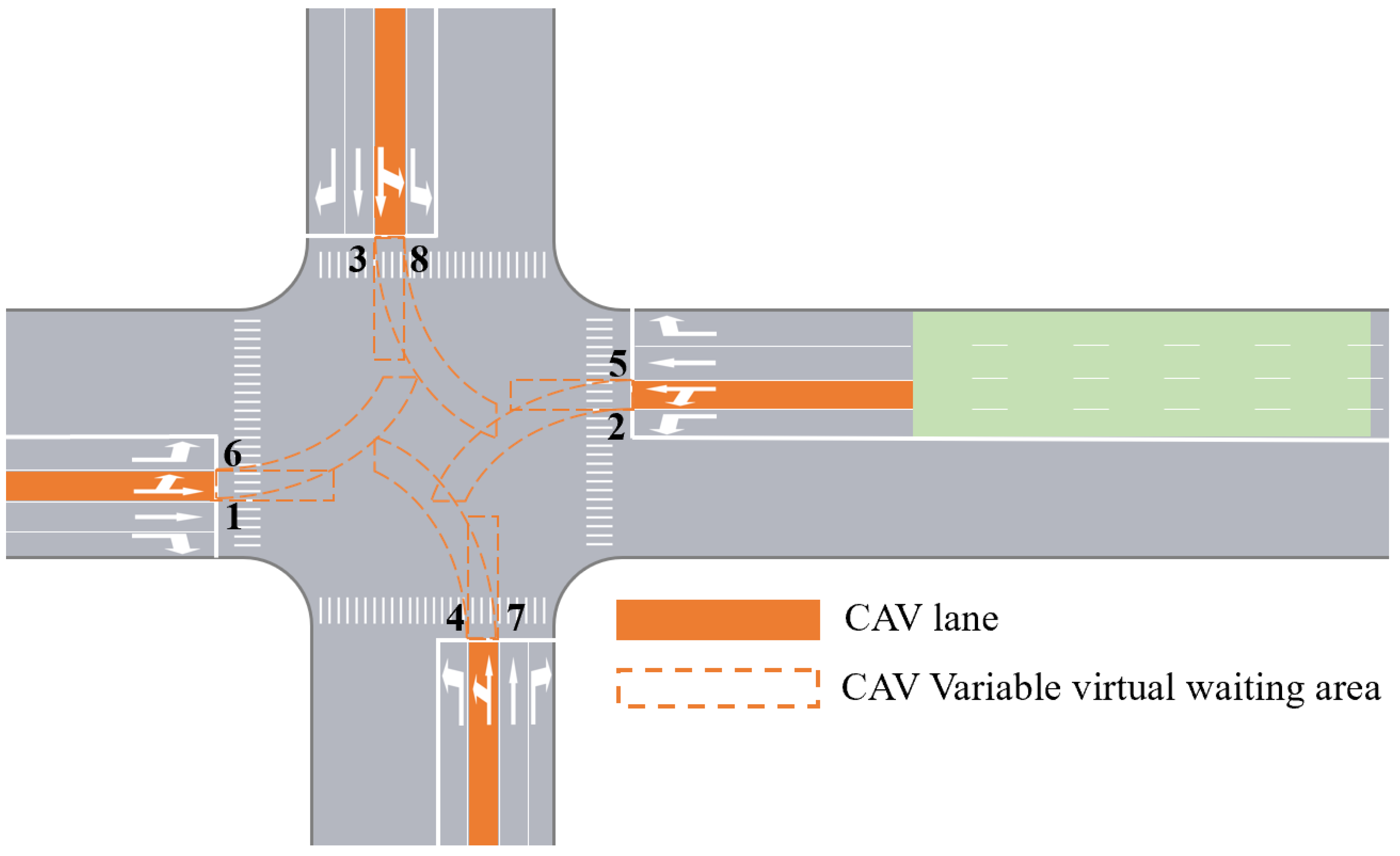
3.2. Variable Virtual Waiting Zone

A variable virtual waiting zone is an area planned inside an intersection in front of a dedicated CAV lane passing zone, divided into a straight virtual waiting zone and a left-turn virtual waiting zone. The actual geography determines the virtual waiting zone length. The principle of setting the virtual waiting zone length is to maximize the use of intersection space value and CAV network connection value without affecting the intersection traffic. Therefore, the maximum length of the straight virtual waiting zone is measured from the intersection stop line along the straight direction to the intersection of the intersecting HV left-turn lane. The maximum length of the left-turn virtual waiting zone is calculated as the distance between the junction stop line along the left-turn direction and the intersection of the intersecting HV straight lane, as shown in Figure 2. A straight-ahead CAV in the designated CAV lane on this side will enter the intersection with the left-turning vehicles at the same time as or with a delay when the intersection’s left-turn signal is in the green phase. The straight-ahead car runs to the straight virtual waiting zone, and when the straight-ahead green light comes on, the CAV passes through the straight virtual waiting zone and enters the intersection in a nonstop manner, finally passing the signal intersection without stopping. Figure 3a is a schematic diagram, and the corresponding phase division diagram is shown in Figure 3b. The intersection lane groups are divided as shown in Figure 2. When the green light for straight-ahead in this lane comes on, in the late green light, the left-turn CAV in the dedicated CAV lane follows the straight-ahead CAV to the left-turn waiting zone in the intersection. When the left-turn green light is on, the CAV passes the left-turn virtual waiting zone and enters the intersection without stopping. The relevant schematic diagram is shown in Figure 3c, and the corresponding phase is shown in Figure 3d. Throughout the process, there is no need to increase the effective green time of the straight-ahead phase or the number of straight-ahead inlet lanes, yet it is equivalent to making the inlet lanes wider. The variable virtual waiting zone makes full use of the intersection area of the intersection, but reduces the signal control time and shortens the entire intersection cycle duration. This type of release can be thought of as exchanging time for space and then space for time, ultimately fulfilling the goal of mutual conversion of space and time while utilizing all of the intersection’s space-time resources.

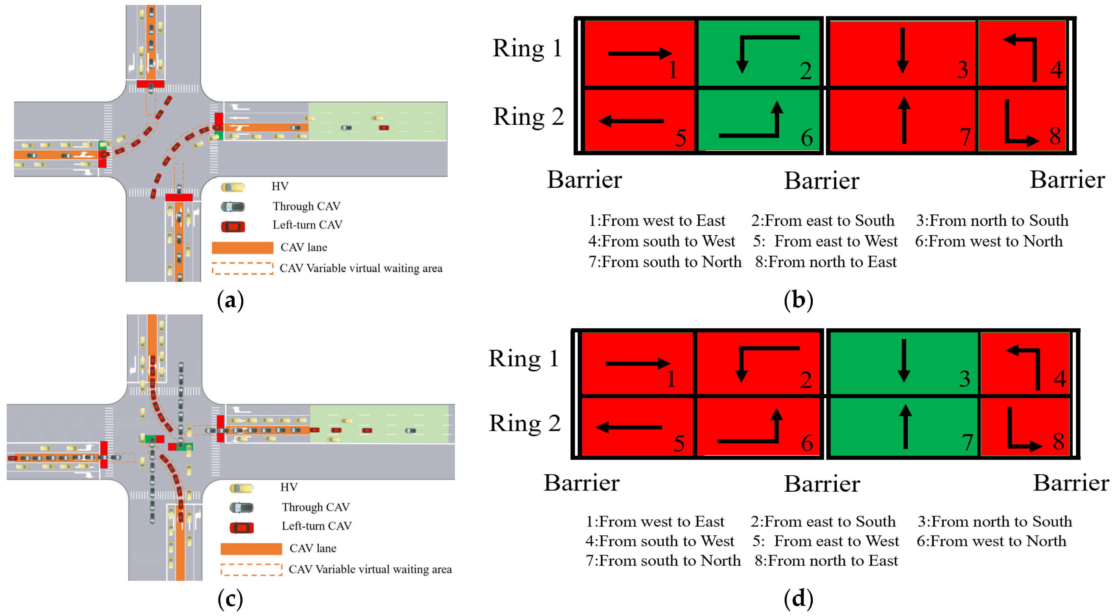
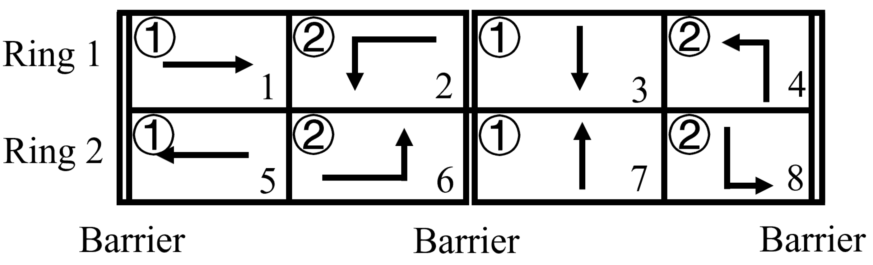
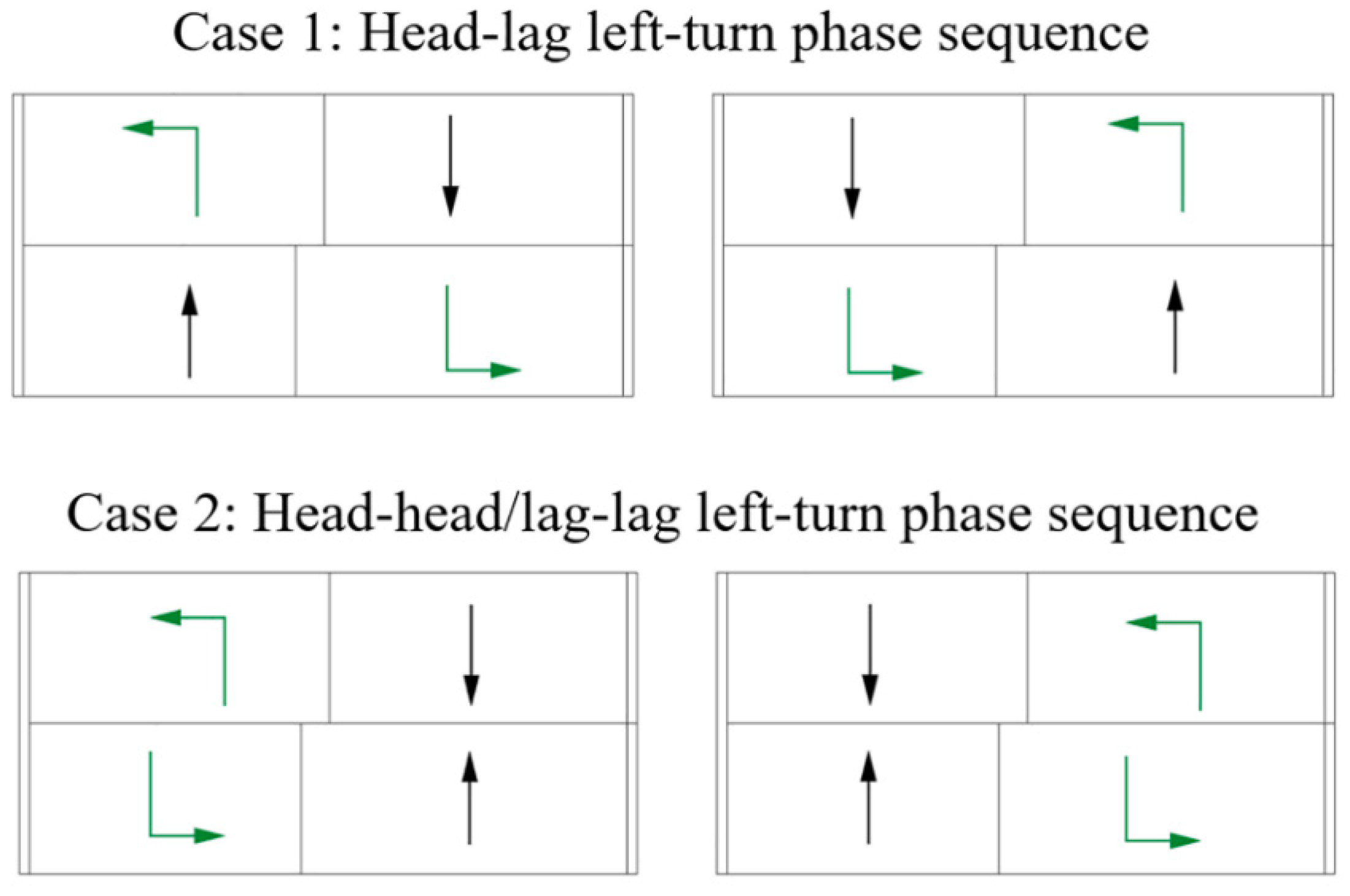
3.3. Intersection Phase Sequence Setting Analysis

In view of a series of HV problems in heterogeneous traffic flow, such as slow signal control response, relatively large headway time distance, and easy traffic violation and secondary parking in the HV left-turn waiting zone, if the left-turn HV and left-turn CAV are set in the same left-turn lane containing the left-turn waiting zone, the CAV network linkage effect will be difficult to utilize. Because CAVs use a dedicated lane, to achieve the overall heterogeneous saturated traffic flow efficiency improvement, this study sets the signal phase of the intersection to a fixed-phase sequence, that is, straight-ahead and then left-turn (Note: This study focuses on the changes brought by the dedicated CAV lane and variable virtual waiting zone on the overall efficiency of the intersection, the question of whether the HV lane is equipped with a waiting area is not considered.). The purpose of this setting is to fully exploit the value of the intersection’s spatial and temporal resources. There is a reason for this: if the left-turn lane turns first, and then the straight-ahead goes, vehicles in the HV straight-ahead lane will be restricted to the stopping line, and only left-turn traffic flow will be available in the intersection, so the intersection space and location resources will not be not fully utilized.

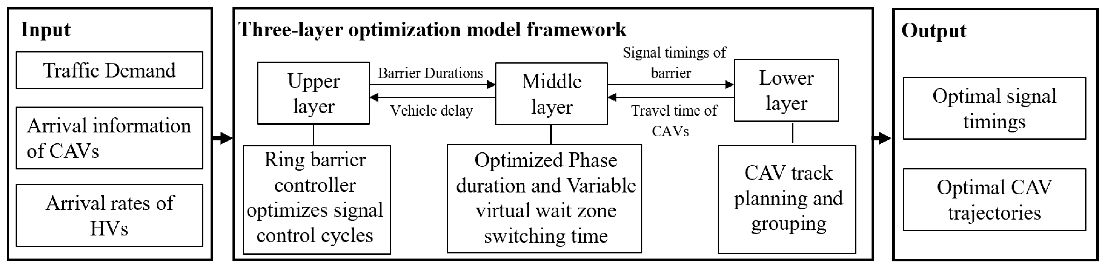
4. Model Formulation

Figure 4 shows the signal control and CAV trajectory optimization model framework based on a variable virtual waiting zone with a dedicated CAV lane proposed in this paper. How CAVs and HVs enter the intersection at future time T is used as the input to the control model. Each CAV can transmit the following information to the control unit through the V2I communication channel: the time of entering the adjustment zone and the direction of travel at the intersection. The control system can also obtain the average arrival rate of each HV in a timely fashion by using the information obtained using roadside sensing equipment.

The model framework includes three layers, which achieve the following: signal timing optimization, variable virtual waiting zone switching time optimization, and CAV trajectory optimization. In order to reduce the time that cars take to cross the intersection, the upper layer of the model dynamically optimizes the barrier duration according to the arrival of vehicles. Using the output from the higher layers, the phase duration of the signal light and the switching time of the variable virtual waiting zone are optimized in the middle layer, and the vehicle delay time calculated by the middle-layer model is fed back to the upper-layer model. Based on the time information transmitted by the middle-layer model, the lower-layer model accurately adjusts a CAV in the passing zone and the variable virtual waiting zone track and simultaneously transfers the CAV travel time to the middle layer. The overall output of the model includes a cross-optimal signal control scheme and CAV trajectory planning.

4.1. Upper-Layer model

Considering the fixed phase sequence in this study, the cycle length and phase duration will be optimized. To facilitate modelling, the NEMA ring barrier structure is adopted, according to Figure 5. Each ring’s and barrier group’s respective 2 phases are indexed as p = 1, 2. For instance, the phases in Figure 5 are indexed as p = 1 for pass directions m of 1, 3, 5, and 7 and as p = 2 for pass directions m of 2, 4, 6, and 8. A urban road traffic system is highly stochastic in nature. The traffic condition of the road network at any time depends not only on the incoming and outgoing traffic volume in the current period, but also on the traffic conditions and control strategies of previous cycles. Since the road network situation changes in each cycle, the traffic conditions of the previous cycles and the current cycle must be considered when optimizing the signal control strategy for the current cycle. The signal control system needs to be discretized into a multistep decision process to better adapt to changes in traffic operating conditions and the environment. Dynamic programming is a method to solve the optimization of the multistep decision process, which can transform the multistep optimal control problem into multiple one-step optimal control problems, and finally achieve optimal process results. Therefore, optimal signal timing in the upper layer is considered a discrete-time dynamic-programming issue.

To prevent a dimension problem in the dynamic planning process, the idea from Ma’s paper [11] is applied in this study. The barrier groups in the NEMA loop are used as the basic stages, and the CAVs and HVs in multiple signal cycles within prediction range T are made to pass the intersection in an optimal way by rolling and repeating barrier group 1 and barrier group 2. This is shown in Figure 6.

The rolling repeated barrier group scheme fully considers the coupling relationship between the traffic situations of the previous and current cycles. As shown in Figure 7, in addressing a real-time traffic control problem, when the suggested model is solved using the most recent traffic state, the signal timing information of the previous two barrier groups is used. In the first barrier group, the optimization program applies the calculated signal timing results to the second signal timing cycle according to the real-time CAV and the predicted HV arrival information. Using Figure 7 as an illustration, throughout the first barrier group of the current signal control cycle, the model optimizes the supplied data using a calculation, and the results of the optimization calculation determine the signal control scheme and CAV trajectory planning of the first barrier group in the second cycle. The CAV of the first barrier group in the second cycle begins to leave the adjustment zone and enter the designated CAV lane once the first barrier group in the first cycle has completed its operation. The real-time entrance speed and the signal control timing are used to change the speed of the CAV queue in the passing zone and the variable virtual waiting zone. Similarly, the second barrier group in the first cycle will affect the second barrier group’s signal control scheme and CAV trajectory planning in the second cycle. In this way, a rolling repetitive barrier group scheme is formed.

The upper-layer control model discretizes the optimal signal duration problem into a time-based dynamic programming problem. The state update frequency is set to $\Delta t$, meaning that the objective function is computed every t seconds, and the total signal control duration is $T$. State $s_j$ at stage j is defined as the sum of time steps allotted up to stage j − 1. The decision variable $u_j$ is used to represent how many time steps were allowed to stage j. The numbers of time steps $U_j^{min}$ and $U_j^{max}$ determine $u_j$:

$$U_j^{min}\le u_j\le U_j^{max}$$

(1)

where $U_j^{min}$ and $U_j^{max}$ are determined by the following:

$$U_j^{min}=\frac{G_{1,j}^{min}+R_{1,j}+G_{2,j}^{min}+R_{2,j}}{\Delta t}$$

(2)

$$U_j^{max}=\frac{G_{1,j}^{max}+R_{1,j}+G_{2,j}^{max}+R_{2,j}}{\Delta t}$$

(3)

where the minimum and maximum green light timings for obstacle group $j$ at phase $p$ are represented by $G_{p,j}^{min}$ and $G_{p,j}^{max}$. $R_{p,j}$ is the yellow- and red-light times for obstacle group $j$ at phase $p$. The term $\Delta t$ is a time step, and $\Delta t$ is set according to the actual situation in this study to ensure that $U_j^{min}$ and $U_j^{max}$ are integers.

The state transfer equation is as follows:

$$s_{j+1}=s_j+u_j$$

(4)

The stage objective function $f_j$ is the minimum intersection delay; the full process objective function $v_j$ is the sum of the stage objective functions.

The core idea of dynamic programming is Bellman’s principle, which seeks the optimal solution through continuous iteration of the objective function, starting from an initial value through the positive sequence to continuously use Bellman’s equation to make corrections, and the optimal policy is derived after calculating the optimal state value by conducting a direct search for the optimal evaluation function.

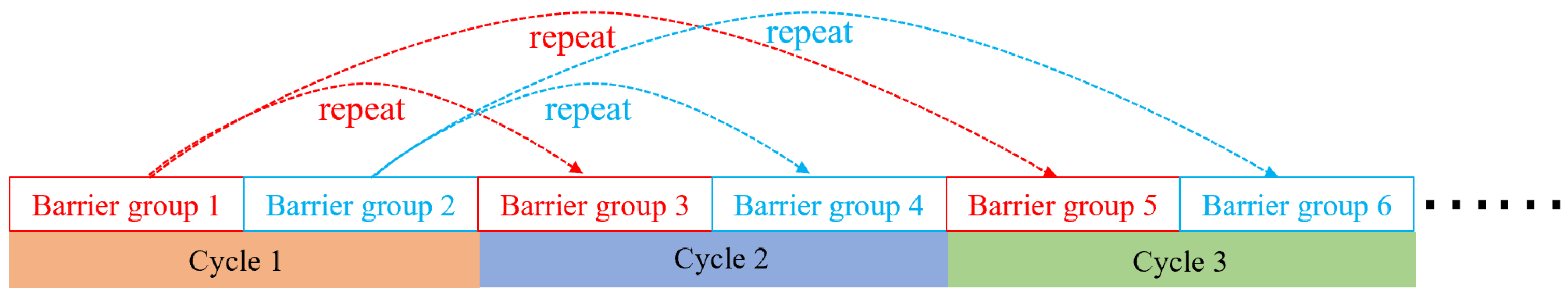
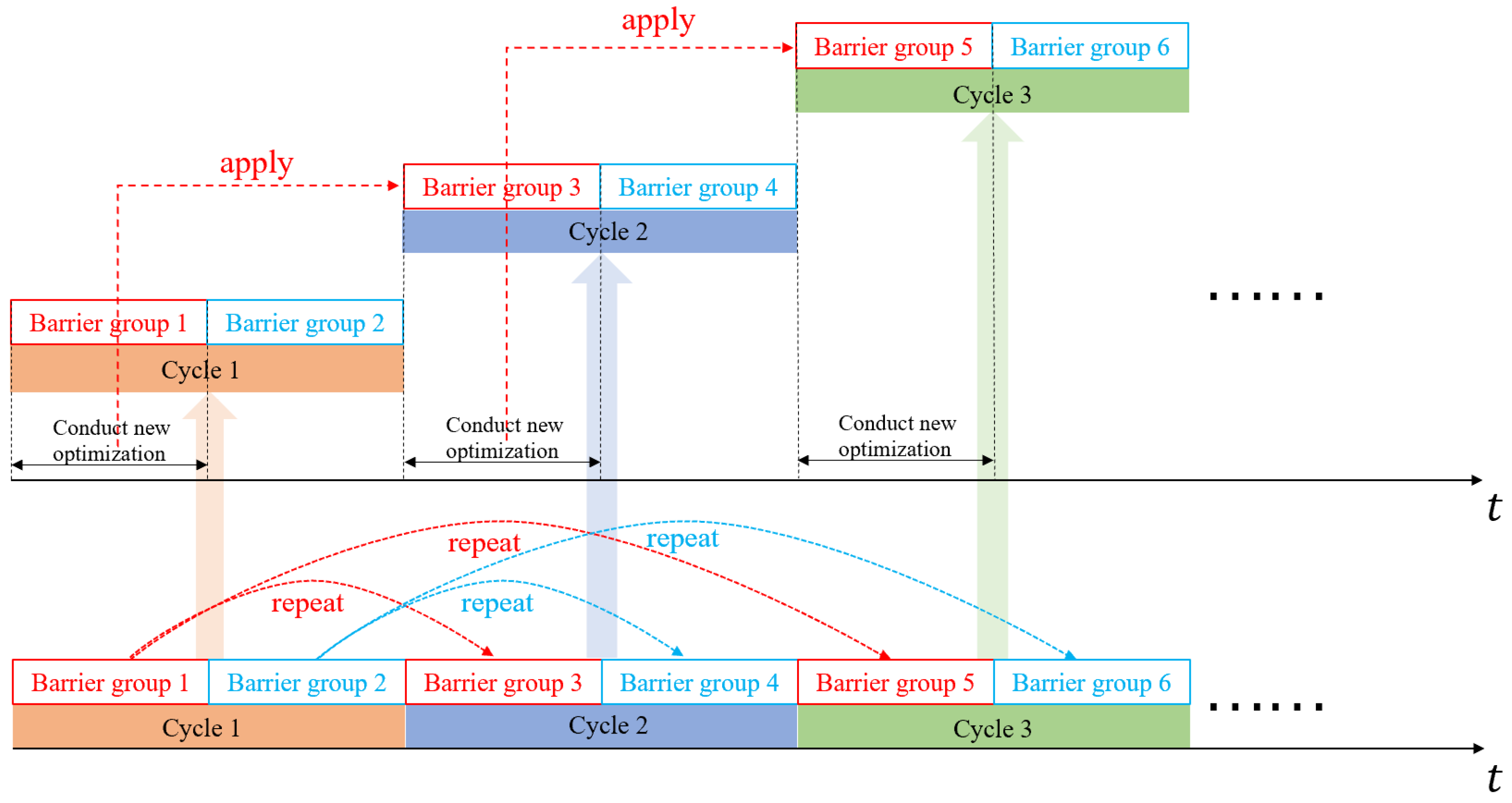
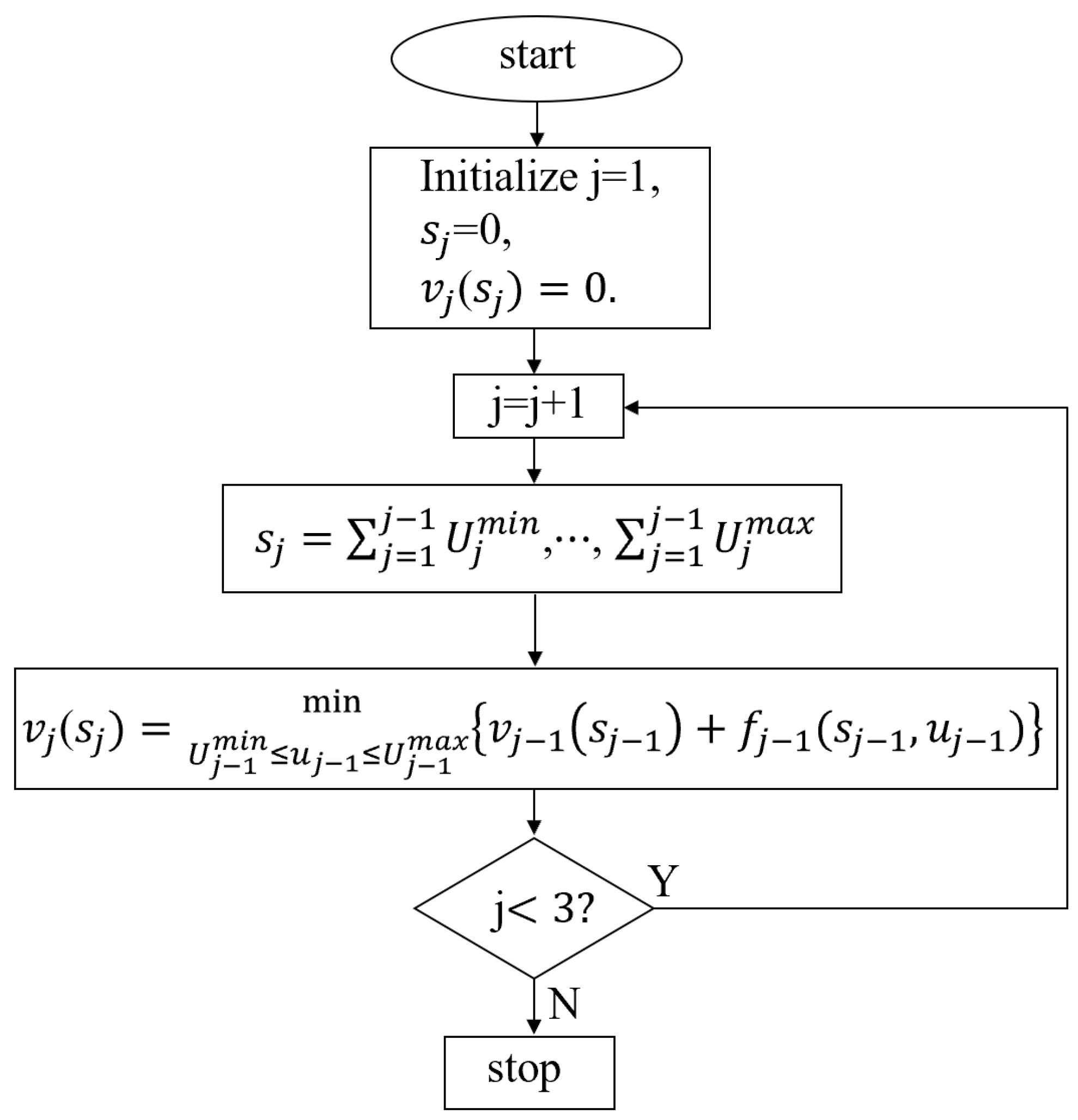
4.1.1. Forwards Recursion

When the signal duration of a cycle is determined, as seen in Figure 6, the total vehicle delay time can be estimated. Figure 8 illustrates the recursive reasoning.

The best choice is represented by $u_{j-1}^{*}\left(s_j\right)$, and the middle-level model’s calculation of $f_j\left(s_j,u_j\right)$ makes use of the phase duration, variable virtual waiting zone switching time, and CAV trajectory optimization.

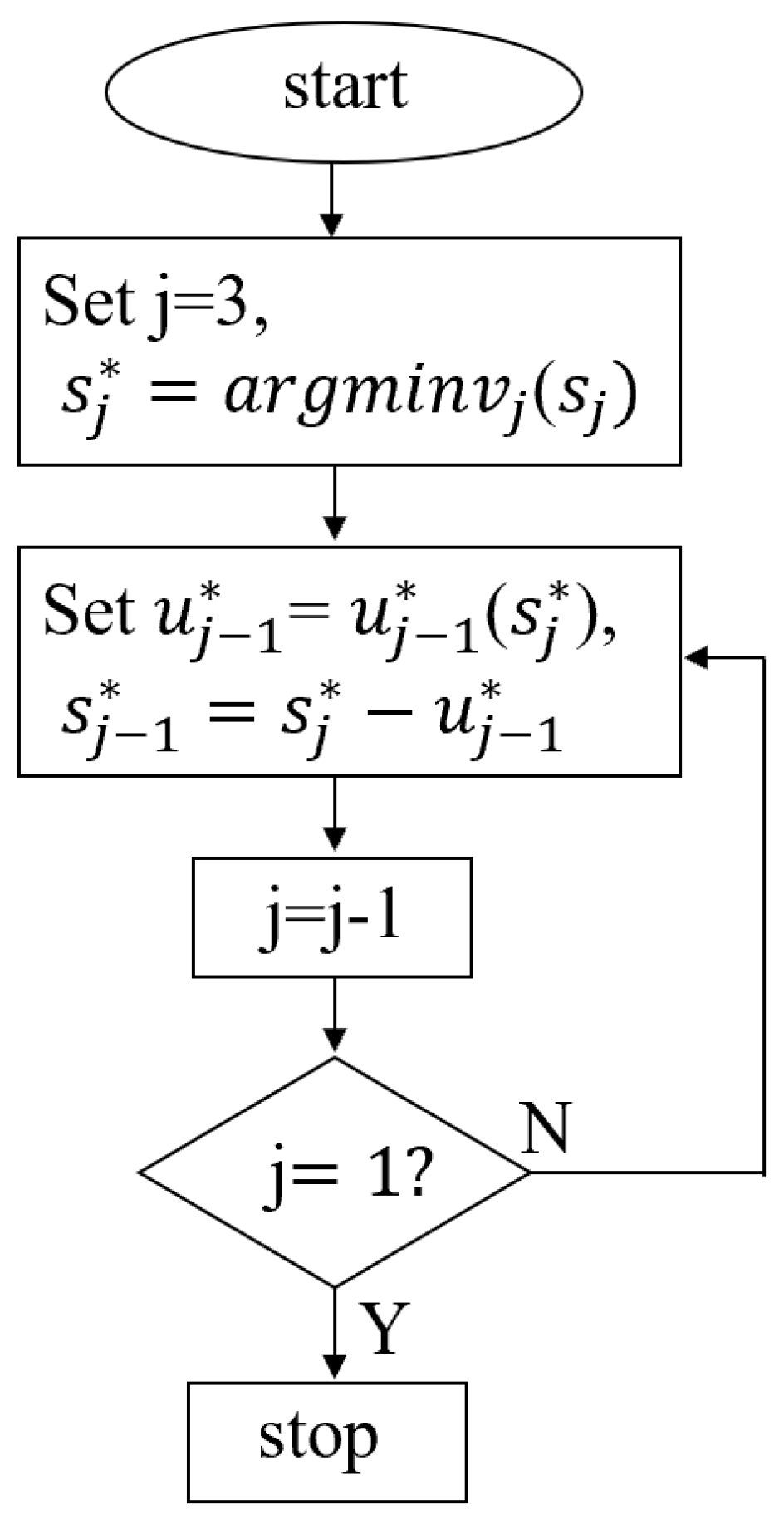
4.1.2. Backwards Recursion

The best choice $u_j^{*}$ at stages 1 and 2 is resolved via backwards recursion in accordance with the dynamic programming principle, according to Figure 9.

4.2. Middle-Layer Model

Based on the data collected from the upper-layer model, the middle-layer model optimizes the phase duration of barrier group $j$ and the holding time of the variable virtual waiting zone. It then gives the upper-layer model the least vehicle delay $f_j\left(s_j,u_j\right)$ for phase $j$.

4.2.1. Human-Driven Vehicle Delays

A moving vehicle’s delay time $d_j^{hm}$ and a stationary vehicle’s delay time $d_j^{hs}$ are both included in the delay time $d_j^h$ of HVs in barrier group $j$:

$$d_j^h=d_j^{hm}+d_j^{hs}$$

(5)

A lane group is described in this work as one or more lanes of the same inlet lane with the same steering function. The term $d_j^{hm}$ is the delay of all human-driven motion vehicles in barrier group $j$, which is equal to the total of the delays of human-driven motion vehicles within each lane group.

$$d_j^{hm}={{\displaystyle \sum }}_{r=1}^2{{\displaystyle \sum }}_p^2{d}_{p,r,j}^h \forall p=1,2;r=1,2$$

(6)

where $d_{p,r,j}^h$ denotes the delay of the barrier group $j$ in the NEMA ring $r$ during the $P$ phase period. It can be reacted to by changing the queue length $l_{p,r,j}$ of the lane group during the phase time, which can be calculated using the following equation:

$$d_{p,r,j}^h={{\displaystyle \sum }}_{t=t_0+s_j+1}^{t_0+s_j+u_j}{l}_{p,r,j}\left(t\right)\Delta t$$

(7)

where $t_0$ is the time step at the beginning of the optimization signal, $l_{p,r,j}\left(t\right)$ is the queue length of the lane group at time $t$ when the phase in NEMA ring $r$ in barrier group $j$ is $P$, and the queue length at time $t$ is jointly influenced by the cumulative vehicle arrival rate ${\tau }_{p,r,j}\left(t\right)$ at time $t$ and the cumulative vehicle dissipation rate ${\theta }_{p,r,j}\left(t\right)$ at time $t$.

$$l_{p,r,j}\left(t\right)=l_{p,r,j}\left(t-1\right)+{\tau }_{p,r,j}\left(t\right)-{\theta }_{p.r.j}\left(t\right) \forall t=t_0+s_j+1,\cdots ,t_0+s_j+u_j$$

(8)

To calculate length $l_{p,r,j}$ at any moment in the signal optimization process, it is necessary to determine length $l_{p,r,j}$ at time $t_0+s_j$, which is calculated using the following formula:

$$l_{p,r,j}\left(t_0+s_j\right)=\{\begin{array}{c}{l}_{p,r,j-1}\left(t_0+s_{j-1}+u_{j-1}\right), if j\ge 2\\ l_{p,r,1}\left(t_0\right)=l_{p,r,1}^0, if j=1\end{array}$$

(9)

where $l_{p,r,1}^0$ is the initial length of the queue at time $t_0$.

The cumulative vehicle arrival rate ${\tau }_{p,r,j}\left(t\right)$ in Equation (8) is the arrival rate of HVs in barrier group $j$ at time step $t$ for NEMA ring $r$ and phase $P$. This value is determined by the arrival rate ${\tau }_m\left(t\right)$ of each moving vehicle in the direction of passage m. The arrival rate ${\tau }_m\left(t\right)$ of each moving vehicle can be divided into a saturated arrival rate ${\tau }_m^s\left(t\right)$ and an unsaturated arrival rate ${\tau }_m^r\left(t\right)$:

$${\tau }_{p,r,j}^s={{\displaystyle \sum }}_m{\tau }_{p,r,j}^m{\tau }_m^s$$

(10)

$${\tau }_{p,r,j}^r={{\displaystyle \sum }}_m{\tau }_{p,r,j}^m{\tau }_m^r$$

(11)

where ${\tau }_{p,r,j}^m$ is defined to be 1 if the moving vehicle crosses the intersection under phase $P$ of ring $r$ of group $j$ and 0 otherwise.

The cumulative vehicle dissipation rate ${\theta }_{p.r.j}\left(t\right)$ in Equation (8) is affected by the queue length and vehicle arrival rate, and considering the phase change, the cumulative vehicle dissipation rate ${\theta }_{p.r.j}\left(t\right)$ is divided into ${\theta }_{1.r.j}\left(t\right)$ and ${\theta }_{2.r.j}\left(t\right)$ by phase:

$${\theta }_{1.r.j}\left(t\right)=\{\begin{array}{l}min\left\{{\tau }_{1,r,j}^s\left(t\right),l_{1,r,j}\left(t-1\right)+{\tau }_{1,r,j}^r\left(t\right)\right\}, if t_0+s_j<t\le t_0+s_j+g_{1,j}\\ 0, otherwise\end{array}$$

(12)

$${\theta }_{2.r.j}\left(t\right)=\{\begin{array}{l}min\left\{{\tau }_{2,r,j}^s\left(t\right),l_{2,r,j}\left(t-1\right)+{\tau }_{2,r,j}^r\left(t\right)\right\}, if t_0+s_j+g_{1,j}+\frac{R_{1,j}}{\Delta t}<t\le t_0+s_j+u_j-\frac{R_{2,j}}{\Delta t}\\ 0, otherwise\end{array}$$

(13)

where $\raisebox{1ex}{$R_{p,j}$}\!\left/ \!\raisebox{-1ex}{$\Delta t$}\right.$ should be an integer and $g_{p,j}$ is the length of the green light during phase switching in phase $j$.

The following equation can be used to determine the delay time $d_j^{hs}$ of a stationary vehicle in stage $j$:

$$d_j^{hs}={{\displaystyle \sum }}_{m=1}^8(1-{{\displaystyle \sum }}_{p=1}^2{{\displaystyle \sum }}_{r=1}^2{\tau }_{p,r,j}^m)d_{m,j}^h$$

(14)

where $d_{m,j}^h$ is:

$$d_{m,j}^h={{\displaystyle \sum }}_{t=t_0+s_j+1}^{t_0+s_j+u_j}{l}_{m,j}\left(t\right)\Delta t, m\in \left[1,8\right]$$

(15)

where l_m,j(t) is:

$$l_{m,j}\left(t\right)=l_{m,j}\left(t-1\right)+{\tau }_m^r\left(t\right) t\in \left[t_0+s_j+1,t_0+s_j+u_j\right]$$

(16)

where $l_{m,j}\left(t_0+s_j\right)$ is:

$$l_{m,j}\left(t_0+s_j\right)=\{\begin{array}{ll}{l}_{m,j-1}\left(t_0+s_{j-1}+u_{j-1}\right), & if j\ge 2\\ l_{m,1}\left(t_0\right)=l_{m,1}^0,& if j=1\end{array}$$

(17)

4.2.2. Connected and Autonomous Vehicle Delays

The delay time $d_j^c$ of the network-linked autonomous vehicles in barrier group j is as follows:

$$d_j^c={{\displaystyle \sum }}_{\omega \in \mathsf{\Psi }}(t_j^{\omega }-t_{free}^{\omega })$$

(18)

$$t_j^{\omega }=t_{before-j}+t_{waiting-j}+t_{normal-j}$$

(19)

$$t_j^{\omega }=t^{\omega }\left({\vartheta }_j,g_j\right),\forall \omega \in \mathsf{\Psi }$$

(20)

where Ψ is the collection of CAVs that arrive at the intersection within anticipated time $T$; $t_{free}^{\omega }$ is the time at which a CAV can pass freely; and $t_j^{\omega }$ is the time at which the CAV actually passes through barrier group $j$. Equation (19) illustrates that this time includes time $t_{before-j}$, which occurs before the CAV enters the virtual waiting zone; time $t_{waiting-j}$, which occurs while it is moving in the virtual variable waiting zone; and time $t_{normal-j}$, which occurs when it crosses the stop line of the variable virtual waiting zone and begins to move inside the intersection (his time is calculated in the lower level trajectory model.). In Equation (20), ${\vartheta }_j$ is the barrier group $j$ phase, $g_j$ is the barrier group $j$ phase duration, and $t^{\omega }$ is the barrier group $j$ signal timing, in the lowest layer model, which is managed by the CAV trajectory planning.

4.2.3. Determination of Variable Virtual Waiting Zone Holding Time

Due to the predefined phase sequence in this study, which is straight forward followed by a left turn, the real vehicle speed $v_{CAV-I}$ at different junctions and the maximum length $S$ of the waiting zone at different intersections are not the same. As a result, the maximum waiting zone length $S$ and the average CAV passage speed in region ${\overline{v}}_{CAV-I-j}$ both influence the variable virtual waiting zone holding time $t_{waiting-j}$:

$$t_{waiting-j}=\frac{S}{{\overline{v}}_{CAV-I-j}}$$

(21)

where $S$ denotes the longest possible length of the intersection’s virtual waiting zone, which is determined by the actual intersection spatial location and vehicle traffic direction, and ${\overline{v}}_{CAV-I-j}$ is the average value of the actual operating speed of CAVs within the variable virtual waiting zone at the intersection in barrier group $j$. ${\overline{v}}_{CAV-I-j}$ is affected by the lower trajectory planning model, and its value size does not exceed the speed limit value of the virtual waiting zone, which is discussed in the subsequent sections.

4.2.4. Signal Constraints

In optimizing the phase duration and the holding time of the variable virtual waiting zone in barrier group $j$, the signal constraints need to satisfy the following equations:

$$G_{p,j}^{min}\le g_{p,j}\Delta t\le G_{p,j}^{max}, \forall p=1,2$$

(22)

$$0<t_{waiting-j}<g_{p,j}$$

(23)

$${{\displaystyle \sum }}_{p=1}^2(g_{p,j}+\frac{R_{p,j}}{\Delta t})=u_j$$

(24)

Equation (22) indicates the minimum and maximum green light duration limits. Equation (23) indicates that the holding time of the variable virtual waiting zone cannot exceed the green light duration of the intersection. Equation (24) shows that $u_j$ is equal to the total of the lengths of the phases in the NEMA loop.

4.2.5. Determination of Variable Virtual Waiting Zone Holding Time

The minimum vehicle delay f_j (s_j,u_j) is calculated differently for stages j = 1 and j = 2 because the model employs a rolling repeated barrier group structure. The lowest delay times $d_1^h$ for HVs and $d_1^c$ for CAVs in the barrier group during stage 1, ($T_1$) are added together when j = 1 to form $f_j\left(s_j,u_j\right)$:

($T_1)$

$$f_1\left(s_1,u_1\right)=\min (d_1^h+d_1^c)$$

(25)

The constraints are Equations (6)–(24), where j = 1.

The minimum delay time $d_j^h$ for HVs and the minimum delay time $d_j^c$ for CAVs in the barrier group during phase $j=2,\cdots ,J$ are added together when $j=2$ to generate the performance function minimum vehicle delay $f_2\left(s_2,u_2\right)$. $J$ is the number of barrier groups that release each HV and CAV during predicted time $T$. The projected demand and signal timeliness of the first two barrier groups define how much it is worth. The following formula, $(T_2)$, is used to determine $f_2\left(s_2,u_2\right)$:

($T_2)$

$$f_2\left(s_2,u_2\right)=\min {{\displaystyle \sum }}_{j=2}^J(d_j^h+d_j^c)$$

(26)

The constraints are Equations (6)–(24), where $j=2,\cdots ,J$.

Due of the small number of participating cars, the mixed-integer nonlinear programming models $T_1$ and $T_2$ are solved using the enumeration approach. The objective function $v_j\left(s_j\right)$ is calculated by feeding $f_1\left(s_1,u_1\right)$ and $f_2\left(s_2,u_2\right)$ into the top-layer model.

4.3. Lower-Layer Model

The middle-layer model provides the signal phase ${\vartheta }_j$, phase duration $g_j$, and holding time $t_{waiting-j}$ information for phase $j$ of the changeable virtual waiting zone. The middle-layer model receives the journey time $t_j^{\omega }$ of the CAVs from the lower-layer model, which performs trajectory planning and travel direction modification for the straight-ahead CAVs and left-turn CAVs in the passing zone and variable virtual waiting zone. In the passing zone and variable virtual waiting zone, the lower-layer model also executes trajectory planning and travel direction adjustment for the straight-ahead CAVs and left-turn CAVs.

4.3.1. CAV Queue Adjustment

When the hold time of every phase in barrier group $j$ is informed state, the passable CAV queue in barrier group $j$ can be determined. Given the preset phase sequence used in this study, the phase sequence setting, or go-straight-ahead and turn-left-behind sequence, is presented in Figure 3.

The straight-ahead and left-turn CAVs are regrouped into straight-ahead CAV groups and left-turn CAV groups in the adjustment zone when the go-straight-ahead and turn-left-behind sequence is utilized. The first vehicle is subject to a different speed restriction, and the CAV queue may wait there until it enters the passing and variable virtual waiting zones. The CAV group turning left then follows the CAV group moving straight into the passing zone. There are two cases, depending on the time of the signal.

Case 1: Two queues. As seen in Figure 10a, a stop-and-wait situation will result if the first left-turn CAV follows the final CAV in the straight-ahead group because of the extended red light time. The group moving straight ahead and the group making a left turn through the intersection can be thought of as two queues in one barrier group to prevent a prolonged stopping time for the left-turn group. The queue can be optimized by Section 4.3.2. The vehicle-following model is determined by Section 4.3.3.

Case 2: A single queue. The first left-turn CAV will not stop at the virtual left-turn waiting zone if it follows the final straight CAV, according to Figure 10b, allowing the entire left-turn CAV group to travel through the junction without stopping. As a result, the convoys making a left-turn and going straight ahead can be thought of as one convoy in one barrier group as they pass through the intersection.

Similar to case 1, the passage time $t_j^{\omega }$ can be calculated for the vehicles in the following queue of the straight-ahead CAV group and the left-turn CAV group. For the CAVs in barrier group $j$ that cannot cross the intersection, the passage time is set to $t_j^{\omega }=t_{free}^{\omega }$.

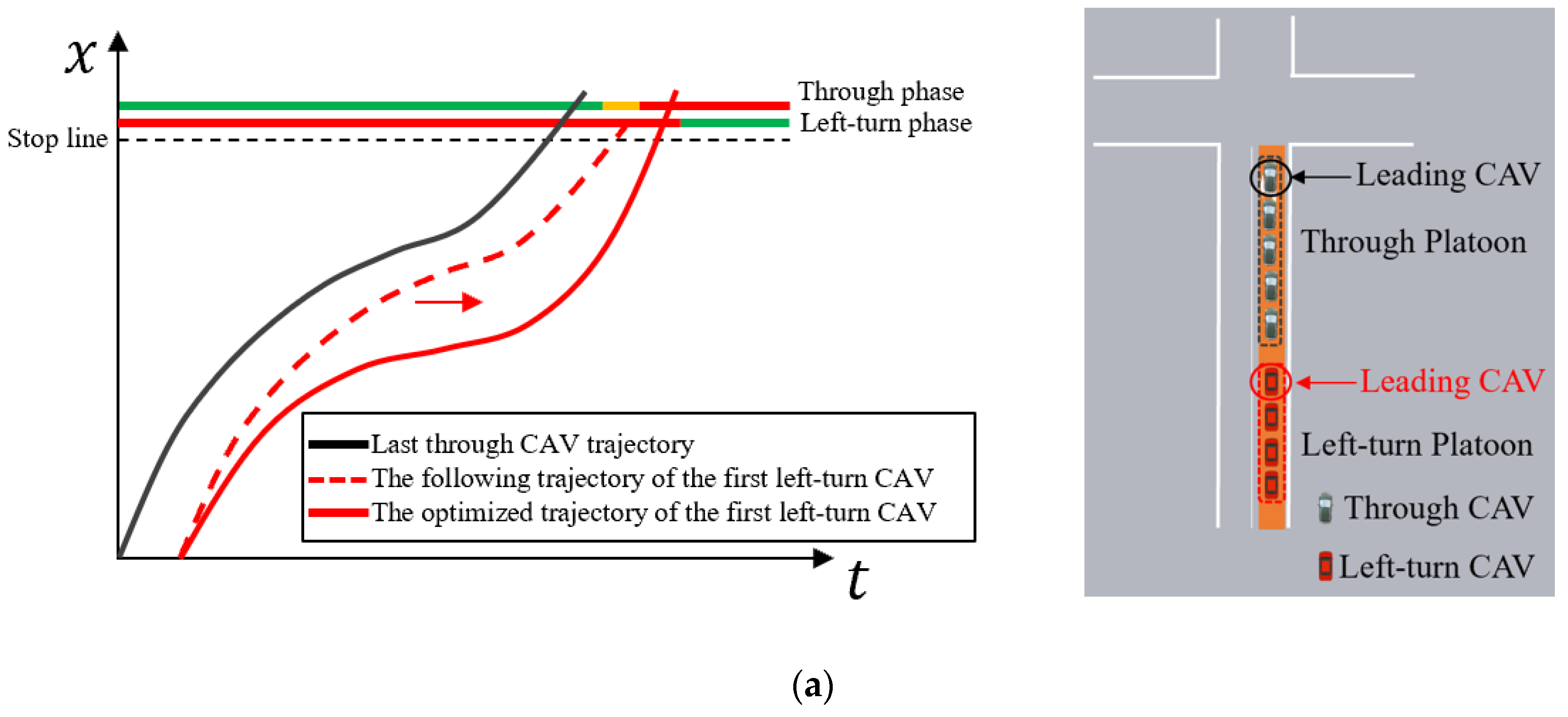
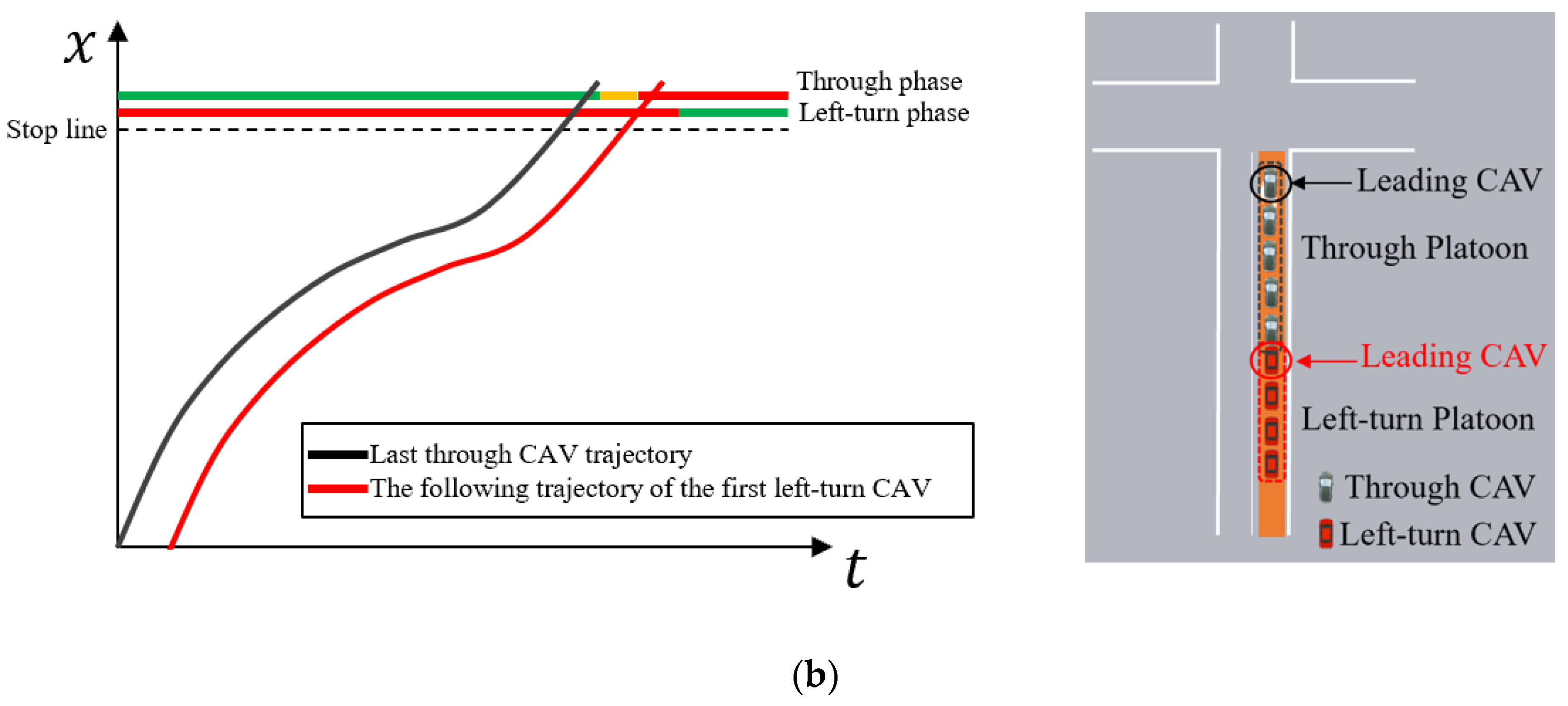
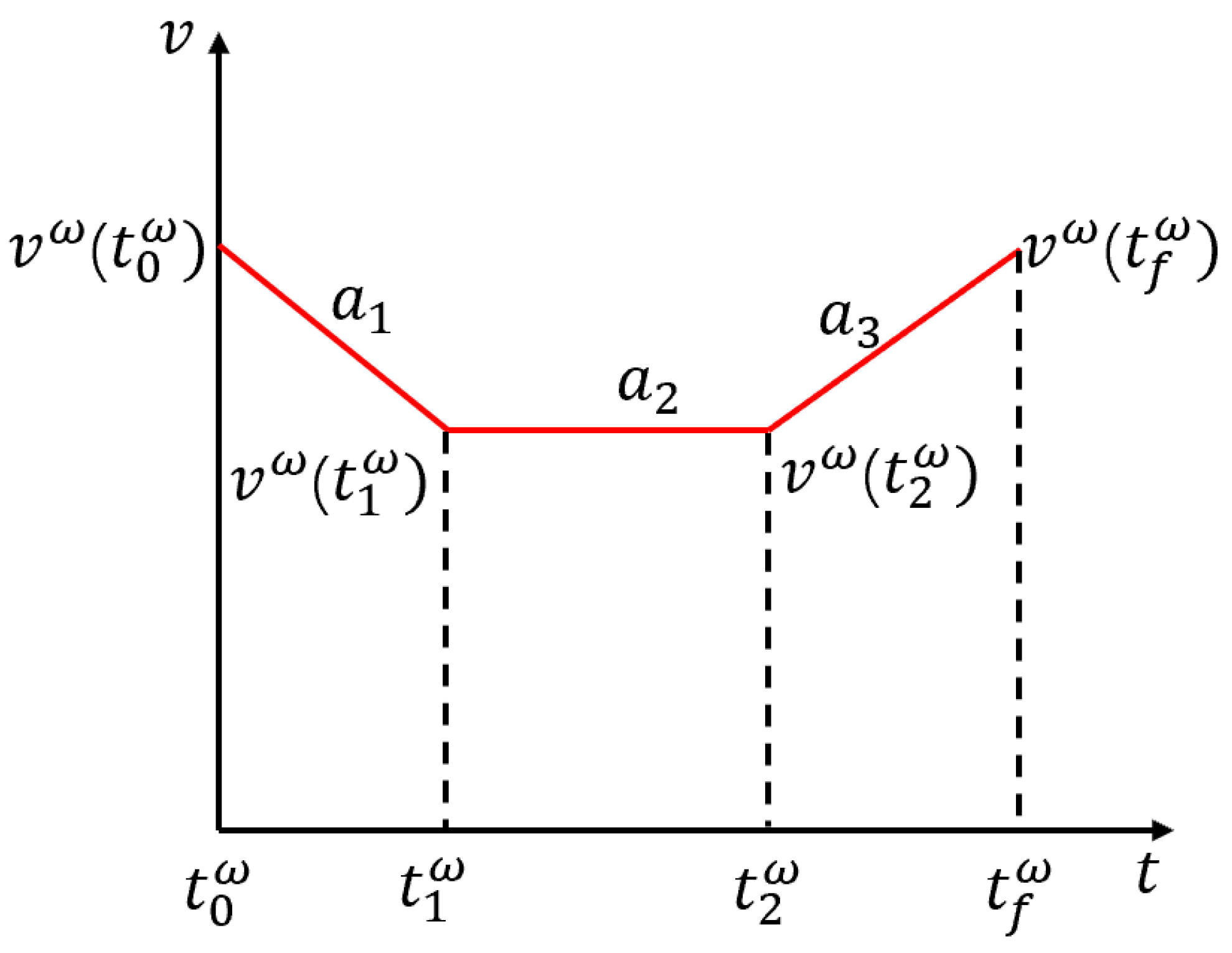
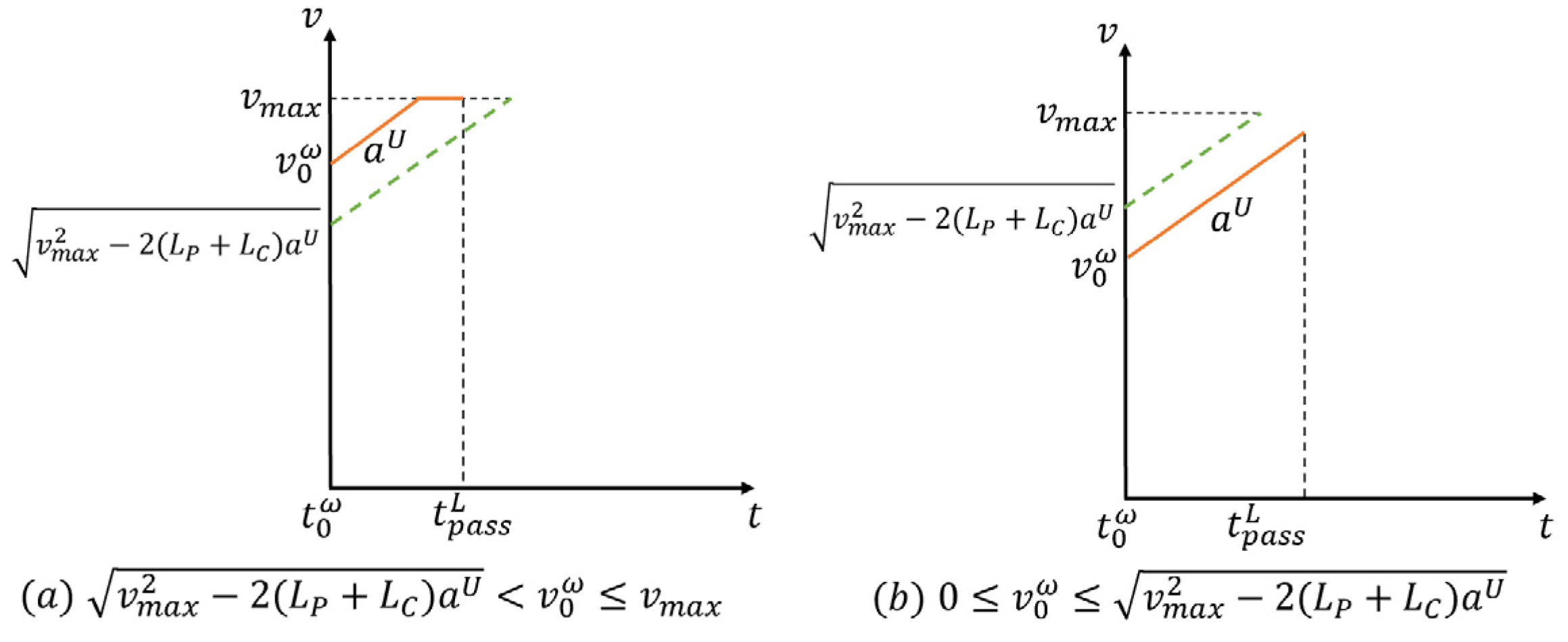
4.3.2. First Vehicle Trajectory Planning in the CAV Queue

The acceleration profile of the first CAV ω at the front of the CAV queue in the passing zone and variable virtual waiting zone is optimized to minimize the trip delay. Similar to the research ideas of Ma and Feng [11,46], this study continues to simplify three-segment trajectory planning, as shown in Figure 11. To ensure that the CAV moves through the passing zone and changeable virtual waiting zone without halting, three portions of the trajectory are identified, with the CAV running at maximum deceleration $a_1$, constant velocity (acceleration of $a_2$), and maximum acceleration $a_3$. $T_3$ is the optimized model.

$(T_3$)

$$min{t}_{pass}^{\omega }$$

(27)

$$max{v}^{\omega }\left(t_{pass}^{\omega }\right)$$

(28)

$s.t.$

$$\{\begin{array}{c}{x}^{\omega }\left(t_0^{\omega }\right)=0\\ v^{\omega }\left(t_0^{\omega }\right)=v_0^{\omega }\end{array}$$

(29)

$$x^{\omega }\left(t_{pass}^{\omega }\right)=L_P+L_C$$

(30)

$$0<v^{\omega }\left(t\right)\le v_{max}$$

(31)

$$a_i^{\omega }\in \left\{a^U,0,a^L\right\},i=1,2,3$$

(32)

$$v^{\omega }\left(t_1^{\omega }\right)-v^{\omega }\left(t_0^{\omega }\right)=\left(t_1^{\omega }-t_0^{\omega }\right)a_1^{\omega }$$

(33)

$$v^{\omega }\left(t_2^{\omega }\right)-v^{\omega }\left(t_1^{\omega }\right)=\left(t_2^{\omega }-t_1^{\omega }\right)a_2^{\omega }$$

(34)

$$v^{\omega }\left(t_{pass}^{\omega }\right)-v^{\omega }\left(t_2^{\omega }\right)=\left(t_{pass}^{\omega }-t_2^{\omega }\right)a_3^{\omega }$$

(35)

$$x^{\omega }\left(t_1^{\omega }\right)-x^{\omega }\left(t_0^{\omega }\right)=\frac{\left(t_1^{\omega }-t_o^{\omega }\right)\left(v^{\omega }\left(t_1^{\omega }\right)+v^{\omega }\left(t_0^{\omega }\right)\right)}{2}$$

(36)

$$x^{\omega }\left(t_2^{\omega }\right)-x^{\omega }\left(t_1^{\omega }\right)=\frac{\left(t_2^{\omega }-t_1^{\omega }\right)\left(v^{\omega }\left(t_2^{\omega }\right)+v^{\omega }\left(t_1^{\omega }\right)\right)}{2}$$

(37)

$$x^{\omega }\left(t_{pass}^{\omega }\right)-x^{\omega }\left(t_2^{\omega }\right)=\frac{\left(t_{pass}^{\omega }-t_2^{\omega }\right)\left(v^{\omega }\left(t_{pass}^{\omega }\right)+v^{\omega }\left(t_2^{\omega }\right)\right)}{2}$$

(38)

$$t_{pass}^{\omega }\ge t_2^{\omega }\ge t_1^{\omega }\ge t_0^{\omega }$$

(39)

$$t_{pass}^{\omega }-t_2^{\omega }=t_{waiting-j}$$

(40)

$$t_{p,j}^g+g_{p,j}\Delta t\ge t_{pass}^{\omega }\ge t_{p,j}^g$$

(41)

where $t_0^{\omega }$ indicates when CAV ω has just reached the passing zone; $t_1^{\omega }$ and $t_2^{\omega }$ indicate the end points of the trajectory of lead CAV $\omega$ during the deceleration phase and the uniform speed phase, respectively; $t_{pass}^{\omega }$ is the moment when lead CAV $\omega$ crosses the stop line ahead of the variable virtual waiting zone; $v^{\omega }\left(t\right)$ and $x^{\omega }\left(t\right)$ are lead CAV ω at time point $t$; $a_i^{\omega }$ is the acceleration of lead CAV $\omega$ during the deceleration phase, the uniform velocity phase, and the acceleration phase; and $a^L$ is the maximum deceleration. The term $a^U$ is the maximum acceleration of lead CAV ω during the acceleration phase; $v_0^{\omega }$ is the initial velocity of lead CAV ω; when the phase index is $P$ in group $j$, the starting time point of CAV ω crossing the intersection is $t_{p,j}^g$; decision variables include $t_i^{\omega }\left(i=1,2\right)$, $t_{pass}^{\omega }$, $a_i^{\omega }\left(i=1,2,3\right)$, $v^{\omega }\left(t\right)$, and $x^{\omega }\left(t\right)$. The passing zone length is $L_P$, and the variable virtual waiting zone length is $L_C$. The other parameters are known.

In Equation (27), the objective function is minimizing $t_{pass}^{\omega }$ since the vehicle arrival time has been determined. It is important to note in this study that, as shown in Figure 12, there may be multiple optimal solutions $t_{pass}^{\omega }$ for the same amount of time to cross the passing zone and the variable virtual waiting zone. For the selection of the optimal solution, preference is given to the trajectory plan that passes the stop line in front of the virtual waiting zone at a higher speed because this will enable a CAV to pass the intersection at a higher safe speed; thus, maximizing the passing speed also becomes the optimization objective, which is Equation (28). The moment $t_0^{\omega }$ at which CAV $\omega$ enters the passing zone is related to the rolling repetition barrier scheme described previously. Equations (29) and (30) define the moment $t_0^{\omega }$ at which CAV $\omega$ enters the passing zone and the moment $t_{pass}^{\omega }$ at which it leaves the stop line of the variable virtual waiting zone. Equation (31) sets the upper and lower speed limits of CAV ω during its operation. Equation (32) constrains the values of acceleration, $a^U,0,a^L$, that is, the maximum deceleration process, the acceleration of the uniform process, and the maximum acceleration of the acceleration process. Equations (33)–(35) define the deceleration, uniformity, and acceleration of the three processes in the velocity–acceleration formula. Equations (36)–(38) define the deceleration, uniformity, and acceleration of the three processes of the velocity-displacement formula. Equation (39) specifies the division of time. Equation (40) is used to calculate the holding time of the variable virtual waiting zone. Equation (41) ensures that CAV ω can cross the junction within the period of time when there is a green light for that phase. It should be noted that the velocity $v_0^{\omega }$ of CAV ω at the time of entering the passing zone is not known, and the magnitude of its value is between the minimum $v_0^L$ and the maximum $v_0^U$. In actual operation, since vehicles prefer to operate at a faster speed, $v_0^{\omega }$ is probably equal to $v_0^U$ in the trajectory planning. The trajectory optimization model $T_3$ can be solved by the method in the Appendix A of this paper, as shown in Figure 12, when the CAV enters the passing zone at time $t_0^{\omega }$. The trajectory planning of the fleet will be adjusted according to the actual entry speed.

4.3.3. CAV Queue-Following Model

Given the simplification of the three-stage trajectory planning in this study, for the sake of simulation, the CAV queue-following model only needs to consider vehicle performance. Therefore, the NGSIM vehicle-following model in Feng’s paper [46] is adopted and described as following:

$$x^{\omega }\left(t+\Delta t\right)=max\left\{x_{\omega }^U\left(t+\Delta t\right),x_{\omega }^L\left(t+\Delta t\right)\right\}$$

(42)

where $x_{\omega }^U\left(t\right)$ and $x_w^L\left(t\right)$ represent the upper and lower limits of $x^{\omega }\left(t\right)$, respectively.

$x_{\omega }^U\left(t+\Delta t\right)$ can be stated using the following equation:

$$\begin{array}{ll}{x}_{\omega }^U\left(t+\Delta t\right)=& min\{x^{{\omega }^{*}}\left(t+\Delta t-{\tau }^{\omega }\right)-l^{{\omega }^{*}}-d_{jam}^{\omega }, x^{\omega }\left(t\right)+v^{\omega }\left(t\right)\Delta t\\ & +a^U\Delta t^2,x^{\omega }\left(t\right)+v_{max}\Delta t, x^{\omega }\left(t\right)+\Delta x^{\omega }\left(t+\Delta t\right)\}\end{array}$$

(43)

$$\begin{array}{l}\Delta x^{\omega }\left(t+\Delta t\right)\\ =\Delta t\left(a^L{\tau }^{\omega }+\sqrt{{(a^L{\tau }^{\omega })}^2-2a^L\left(x^{{\omega }^{*}}\left(t\right)-x^{\omega }\left(t\right)-l^{{\omega }^{*}}-d_{jam}^{\omega }-\frac{{(x^{{\omega }^{*}}\left(t\right))}^2}{2a^L}\right)}\right)\end{array}$$

(44)

where the CAV convoy’s lead vehicle is ${\omega }^{*}$, CAV $\omega$’s reaction time is ${\tau }^{\omega }$, the distance between CAV $\omega$ and other CAVs is $d_{jam}^{\omega }$, $l^{{\omega }^{*}}$ is the vehicle length of CAV vehicle ${\omega }^{*}$, $a^U$ is the maximum CAV acceleration, the greatest headway safety time distance that CAV $\omega$ must travel to avoid a collision at time $t+\Delta t$ is $\Delta x^{\omega }\left(t+\Delta t\right)$, and $a^L$ is the maximum CAV deceleration.

The lower limit distance $x_{\omega }^L\left(t\right)$ is related to the current position that prevents the CAV from backing up and the maximum acceleration/deceleration of the vehicle, so that $x_{\omega }^L\left(t+\Delta t\right)$ can be expressed as follows:

$$x_{\omega }^L\left(t+\Delta t\right)=max\left\{x^{\omega }\left(t\right),x^{\omega }\left(t\right)+v^{\omega }\left(t\right)\Delta t+a^L\Delta t^2\right\}$$

(45)

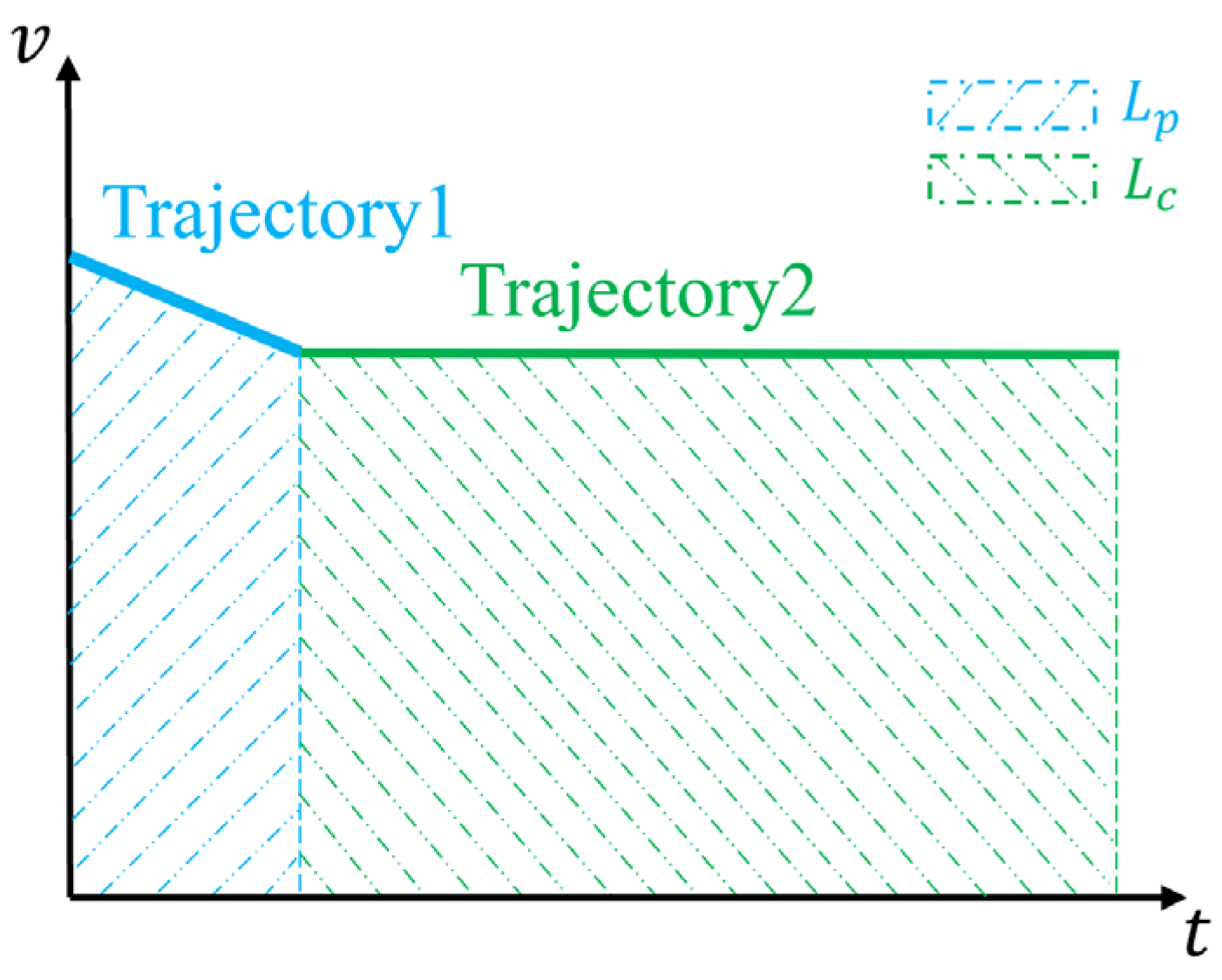
4.4. Determination of the Passing Zone Length

It is possible to regulate the moment the CAV queue enters the adjustment zone’s passing zone. If the CAV queue enters the passing zone within limited speed range $\left[v_0^L,v_0^U\right]$, the size of the passing zone must be set reasonably in conjunction with the length and direction of the variable virtual waiting zone in order to protect the CAVs’ capacity to pass the stop line of the variable virtual waiting zone without stopping, all the while maintaining the speed limit. In this study, we refer to Feng’s research results on the impact of travel distance on the design of CAV trajectories. It should be emphasized that CAV queue adjustment in the adjustment zone, especially lane-changing behaviour, crowds the HV lane under oversaturated traffic conditions, and thus may cause delays in HV passage. The adjustment zone will lead to inaccurate HV delay prediction in 4.2.1, especially close to the HV stop line. The CAV trajectory planning approach, however, may and will lead to an unrealistic passing zone. Therefore, the following equation can be used to determine the passing zone’s maximum length $L_{P-max}$:

$$L_{P-max}=\frac{v_{max}^2-v_0^{L^2}}{2a^U}+\left(X_j^{min}-\frac{v_{max}-v_0^L}{a^U}\right)v_{max}-L_C$$

(46)

This research focuses on cooperative control of signals and car movements at lone intersections, and makes the assumption that there are enough lane lengths for zoning in the problem at hand. The minimum passing zone length must also be quantified in addition to the maximum passing zone length study. If the passing zone is long enough to provide the proper trajectory planning model, the CAV queue should be allowed to pass without halting at the stop line in front of the variable virtual waiting zone. Equation (47) can be used to express $L_{P-min}$:

$$L^{min}=\frac{v_0^{U^2}}{2\ast a^L}$$

(47)

5. Simulation Study

5.1. Simulation Settings

To systematically analyse the properties of the recommended model, a single classic four-way intersection with a left–centre–right direction of travel is used, as shown in Figure 2, where there are no traffic lights to manage right-turning vehicles. The passing zone is 500 m long, and the variable virtual waiting zone length is 20 m for the straight-ahead and 35 m for the left-turn. Combined with the three-layer optimization model introduced in Chapter 4, the shortest period of time during which there is a green light $G_{p,r,j}^{min}=$15 s, the longest possible period of time for the green $G_{p,,j}^{max}=$ 40 s, and the spacing time $R_{p,j}=$ 5 s are set in the upper-layer model. In the model of the middle layer, the saturated left-turn HV flow (when m is 2, 4, 6, and 8) is 1550 veh/h, and the direct saturated flow of HVs (when m is 1, 3, 5, and 7) is 1650 veh/h. In the model of the base layer, the maximum rate of acceleration $a^U$ of CAVs is $2 \mathrm{m}/{\mathrm{s}}^2$, the greatest rate of slowdown $a^L$ is $-2 \mathrm{m}/{\mathrm{s}}^2$, the maximum CAV speed limit is 14$\mathrm{m}/\mathrm{s}$, the total distance $d_{\omega }^{jam}$ and body-fixed length $l_{\omega }$ of the front end are 6 m, and the car’s response time is 0 s. The beginning speed of the first CAV stepping into the passing zone is generated at random between $v_0^L$ (3 m/s) and $v_0^U$ (14 m/s). VISSIM 4.3 (PTVAG, 2008) was selected as the simulation software, and Wiedermann 74 was chosen as the CAV-following and lane-change models, which can collect the HV driving behaviour in the simulation.

Each arm sees an average of 2250 vehicles every hour. The vehicle arrivals during the simulation are divided into uniform distribution and Poisson distribution, where the proportions of vehicles turning left, right, and straight ahead are, respectively, 0.4, 0.2, and 0.4, and 50% of the population are CAVs. The straight and left-turn ahead CAVs operate in a dedicated CAV lane consisting of a passing zone and a variable virtual waiting zone. The prediction range $T$ is set to 2 min. The sake of simplicity and the frequency of HV arrival obtained from the previous prediction within the prediction horizon $T$ are considered as the average HV arrival rate. The arrival information of each CAV within the predicted range is available through communication methods.

The model for managing traffic at a single crossroads with a dedicated CAV lane in a mixed-traffic environment based on shared-phase dedicated lanes (SPDL) proposed by Ma [11] is used as a benchmark for evaluation. The model proposes that CAVs use a dedicated CAV lane in a queue. The model plans the intersection signal phase and signal duration as well as the vehicle trajectory collaboratively, as shown in Figure 13; however, the model does not fully utilize the space within the intersection area.

A desktop PC equipped with an Intel 2.6 GHz CPU and 16 GB of RAM is used for all experiments in this study, and the simulation model is constructed in Python 3.7.4. Five threads are utilized in parallel computation to increase the computing performance. During the simulation of each trial, five random seeds are employed to account for the ambiguity of vehicle arrival and HV driving behaviour. With a forecast time T of 2 min and a time step $\Delta t$ =1 s, every simulation was run for 1000 s.

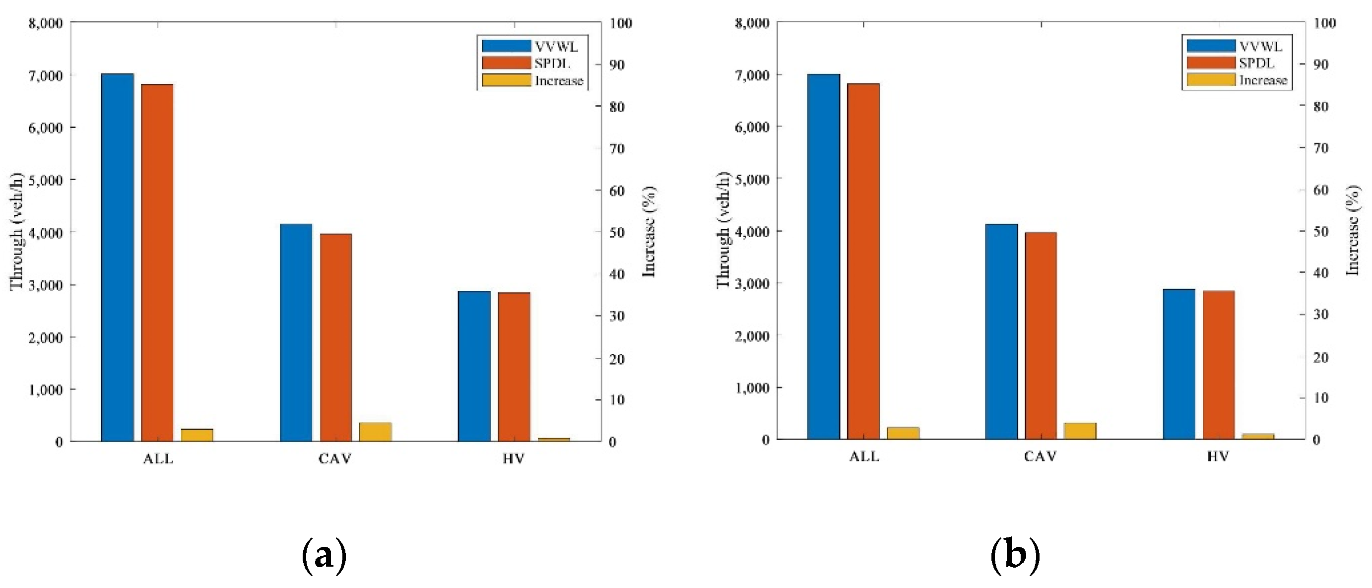
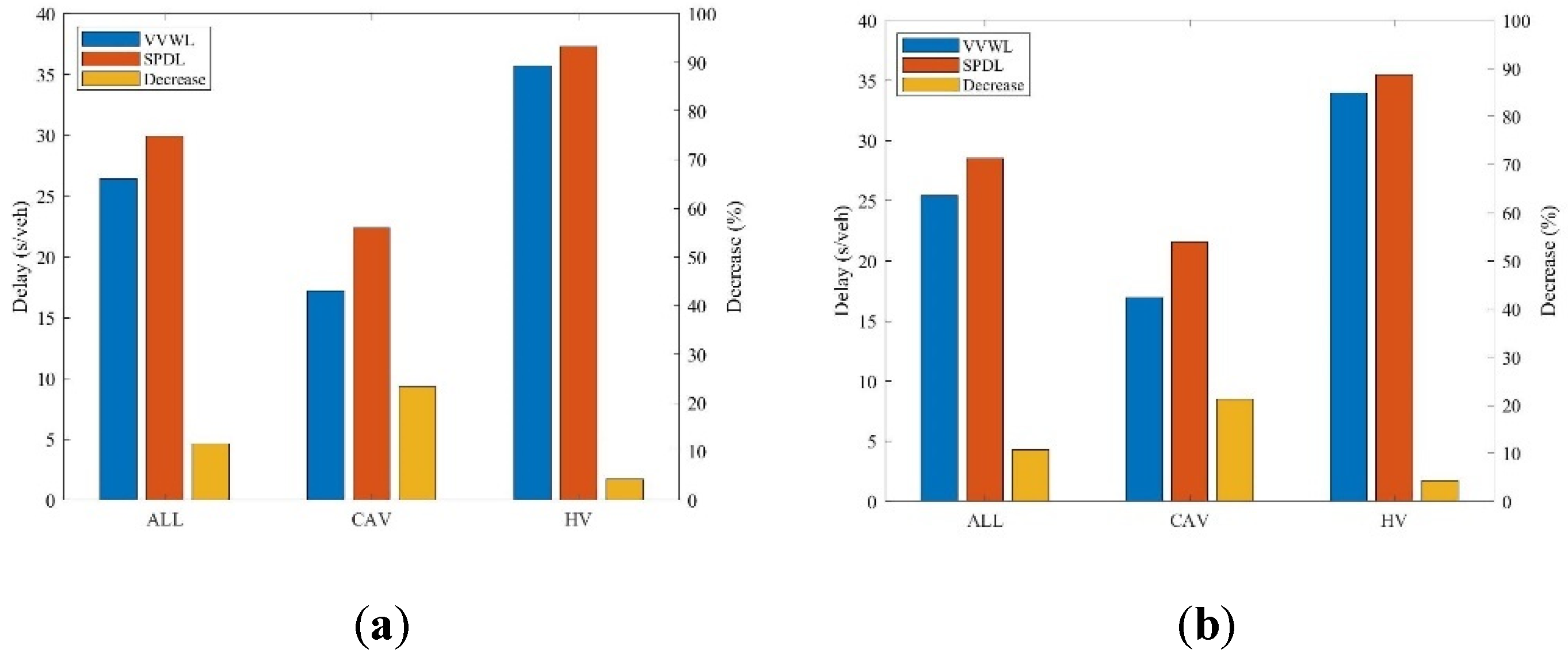
5.2. Simulation Results and Analysis

This study is concerned with the cooperative control problem of oversaturated heterogeneous traffic flow at a single intersection. Therefore, minimizing delay and maximizing throughput are used as metrics to evaluate and analyse the performance advantages and disadvantages between the oversaturated heterogeneous traffic flow signal control model (VVWL) based on the variable virtual waiting zone of the dedicated CAV lane and the SPDL-based control model suggested in this study. As seen in the preceding section, the optimal control objective in this study is the minimum vehicle delay, which is equivalent to the period that separates the moment that a vehicle actually travels from the time that it is free to move. The simulation results are displayed in Figure 14 and Figure 15.

Figure 14 compares the vehicle volumes of heterogeneous traffic flows under control based on both VVWL and SPDL in relation to both uniform and Poisson distributions. As seen in Figure 14a, the VVWL-based control mode increases the total volume of all vehicles, CAVs, and HVs, respectively, by 3%, 4.5%, and 0.9%, as opposed to the control based on SPDL mode, when a uniform distribution of vehicles arrive at the intersection. As seen in Figure 14b, whenever a Poisson distribution of vehicles arrive at the crossroads, the vehicle capacity increases by 2.8%, 4%, and 1.2%, respectively. The proposed variable virtual waiting zone helps to improve the intersection capacity and has a greater impact on the improvement of CAV capacity. The main reason to explain this is that the proposed variable virtual waiting zone allows more CAVs into the intersection at the same time, which increases the capacity of CAVs in the same signal control cycle, and this advantage will be more obvious if the demand for passing vehicles is higher.

Figure 15 compares the average vehicle passage delay of heterogeneous traffic flow under control based on both VVWL and SPDL from both the uniform and Poisson distribution perspectives. The results in Figure 15a show that when all types of vehicles conform to a uniform distribution, all vehicles’ delays are reduced by the control based on VVWL mode, CAVs, and HVs by 11.5%, 23.2%, and 4.3%, respectively, compared to the control mode that is based on SPDL. The results in Figure 15b show that when all types of vehicles conform to a Poisson distribution, the control based on VVWL mode cuts down on all vehicles’ delays by 10.7%, 21.3%, and 4.4% for CAVs and HVs, respectively, in contrast to the control mode based on SPDL. Obviously, the proposed variable virtual waiting zone effectively reduces the vehicle delays regardless of the distribution, and the CAV delay reduction is more significant. The main reason is that the variable virtual waiting zone improves the average speed of CAVs passing through the intersection. For the sake of illustration, the complete process of CAVs passing through the intersection is taken as an example, as shown in Figure 16, because the variable virtual waiting zone is inside the intersection. When CAVs are performing trajectory planning, the passing zone and the variable virtual waiting zone are connected, causing the average speed of CAVs in the variable virtual waiting zone to be high relative to the average speed after leaving the variable virtual waiting zone; as a result, CAVs traverse the intersection at a faster average speed and experience less traffic congestion.

5.3. Sensitivity Analysis

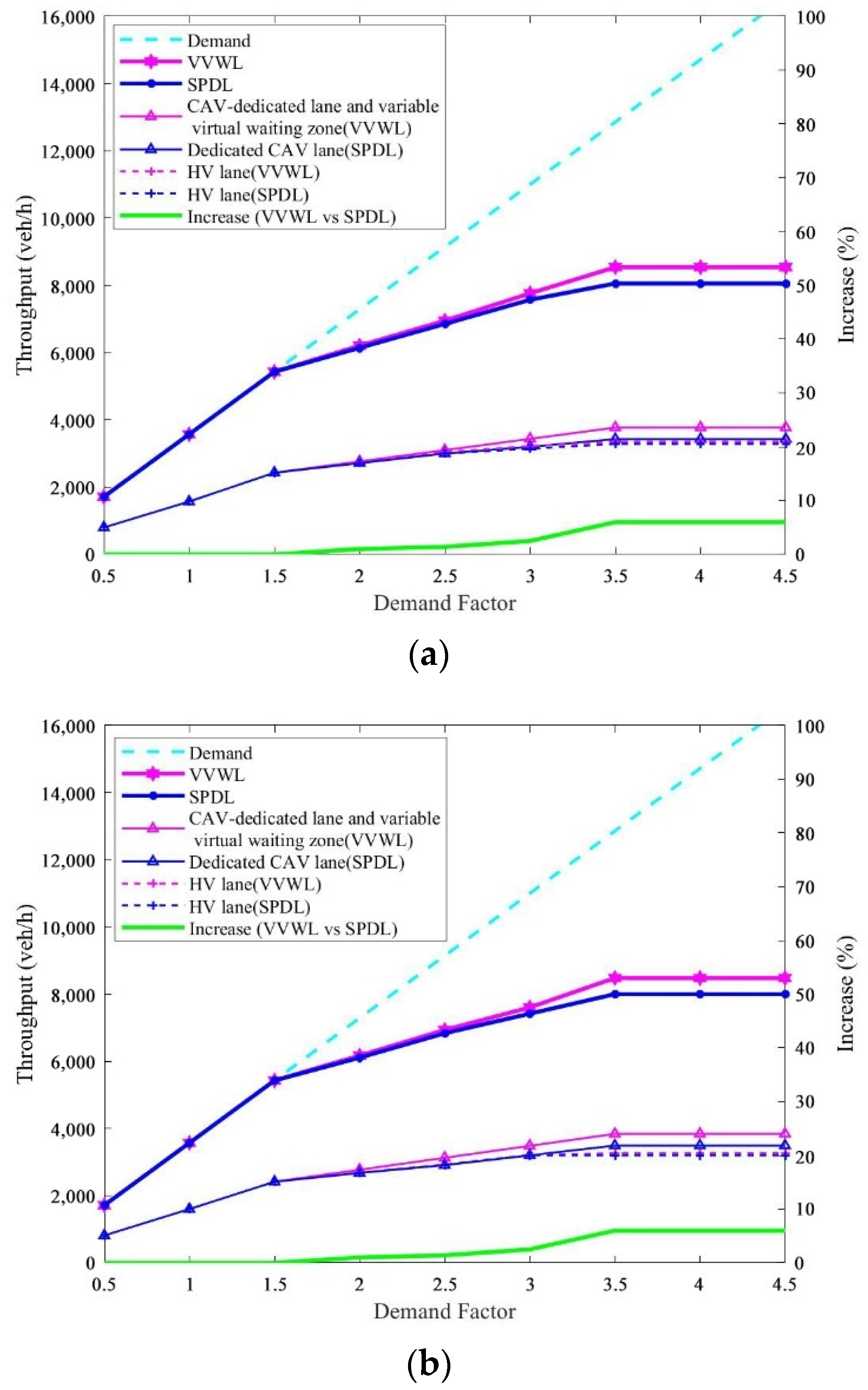
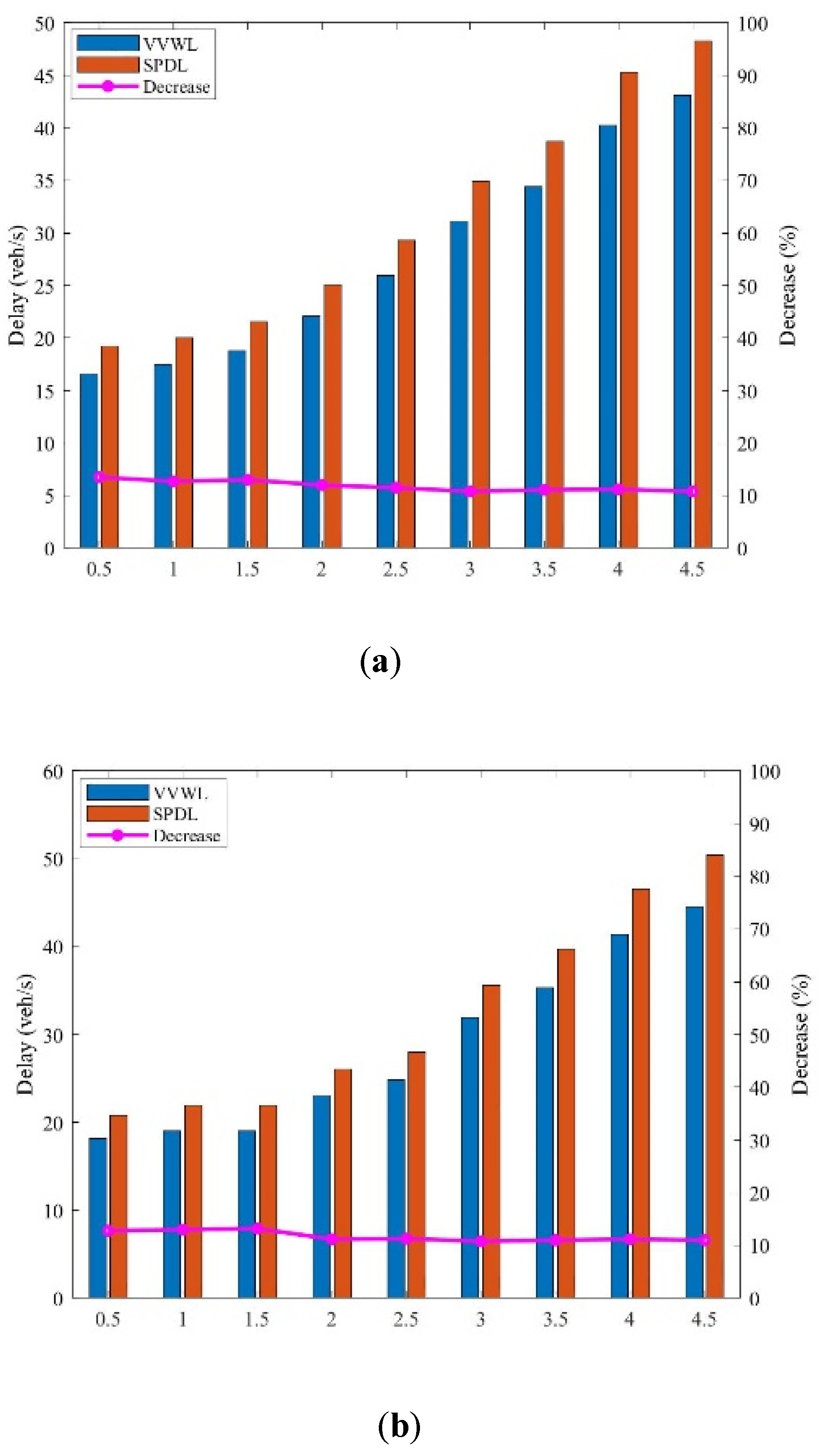
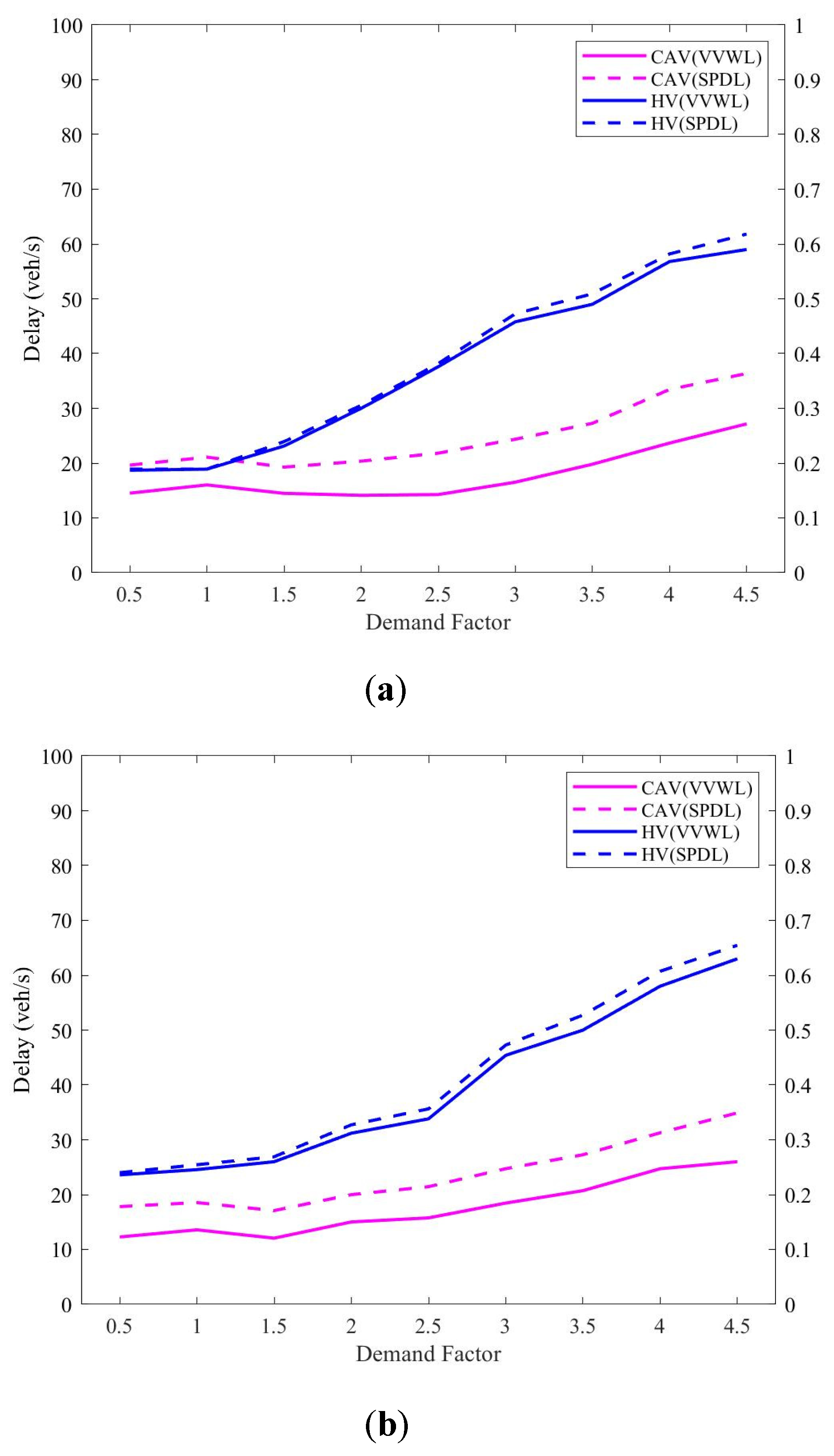
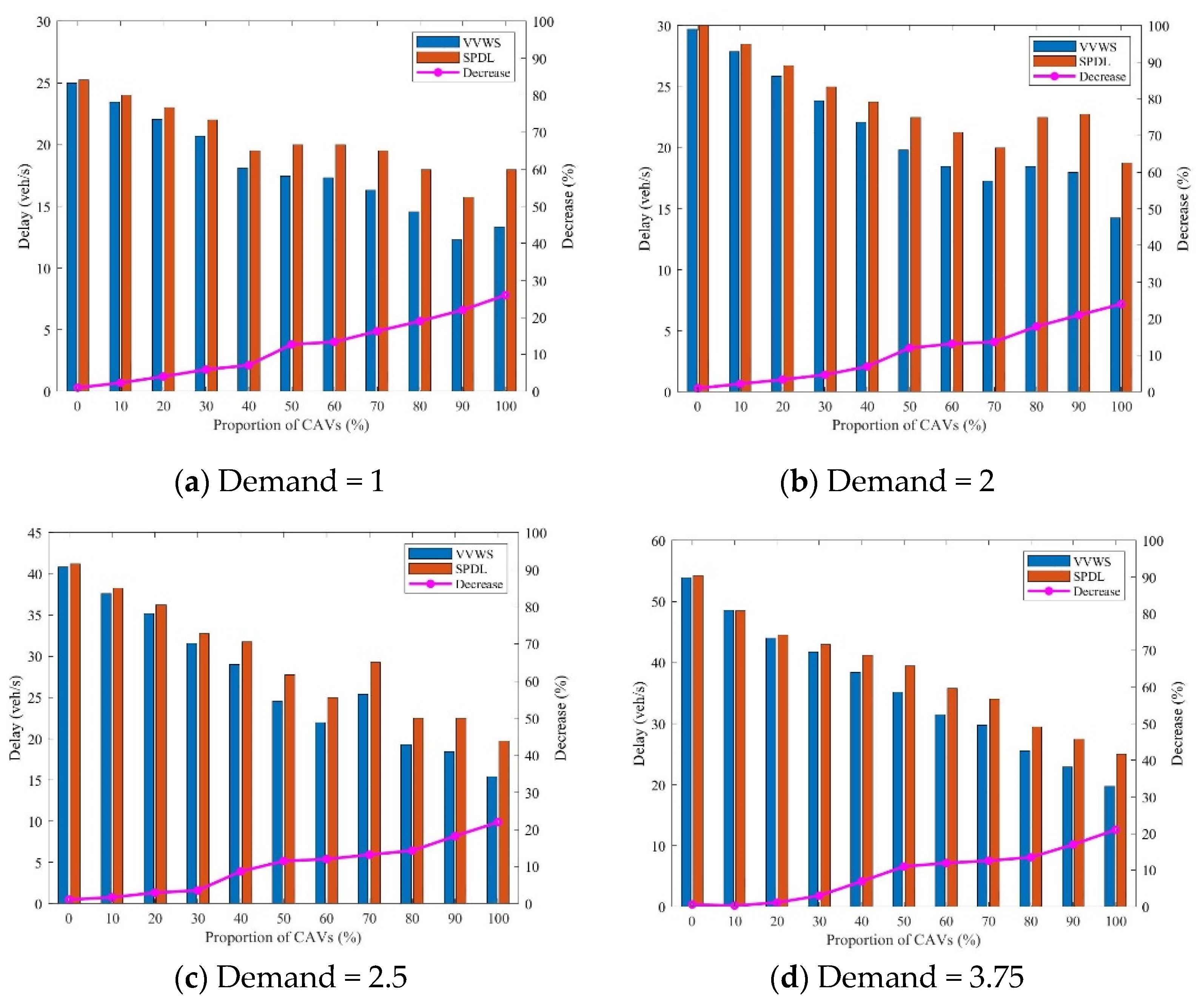
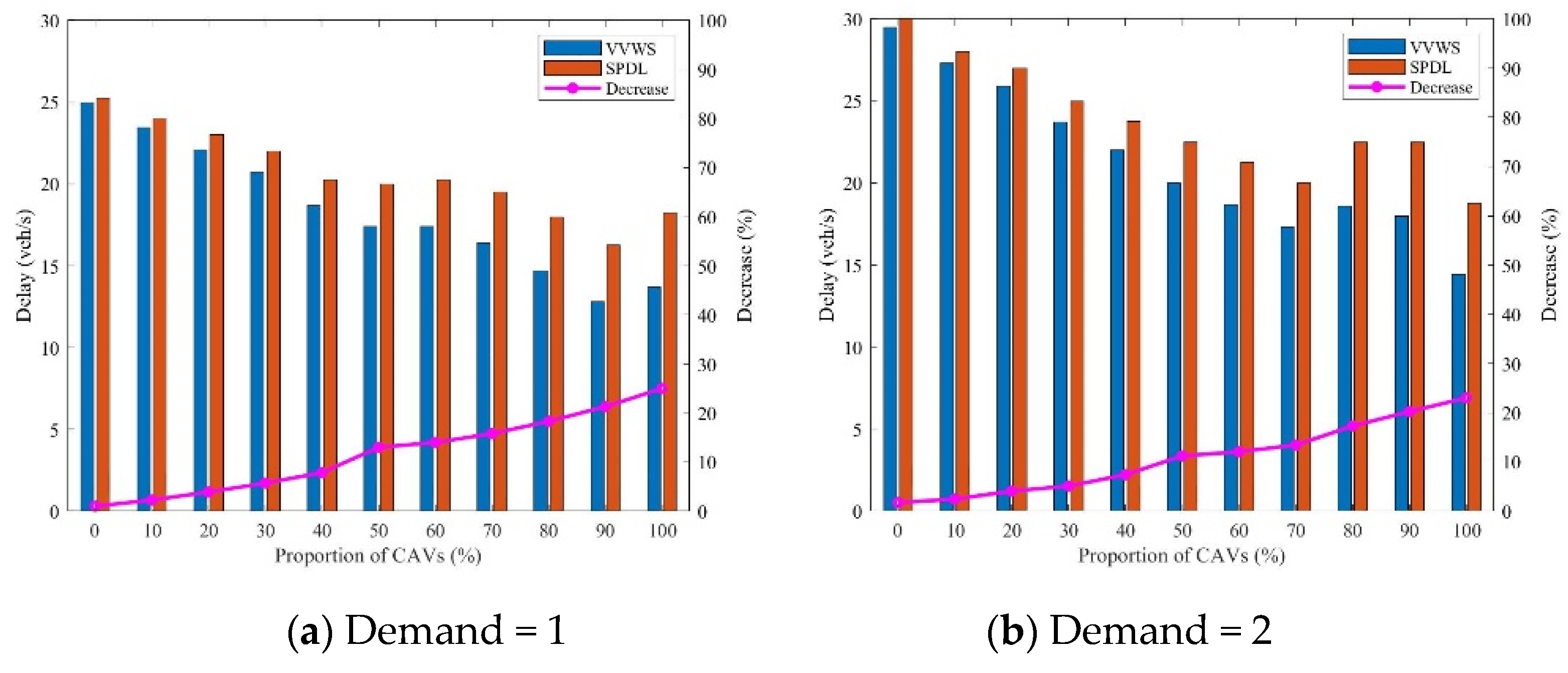
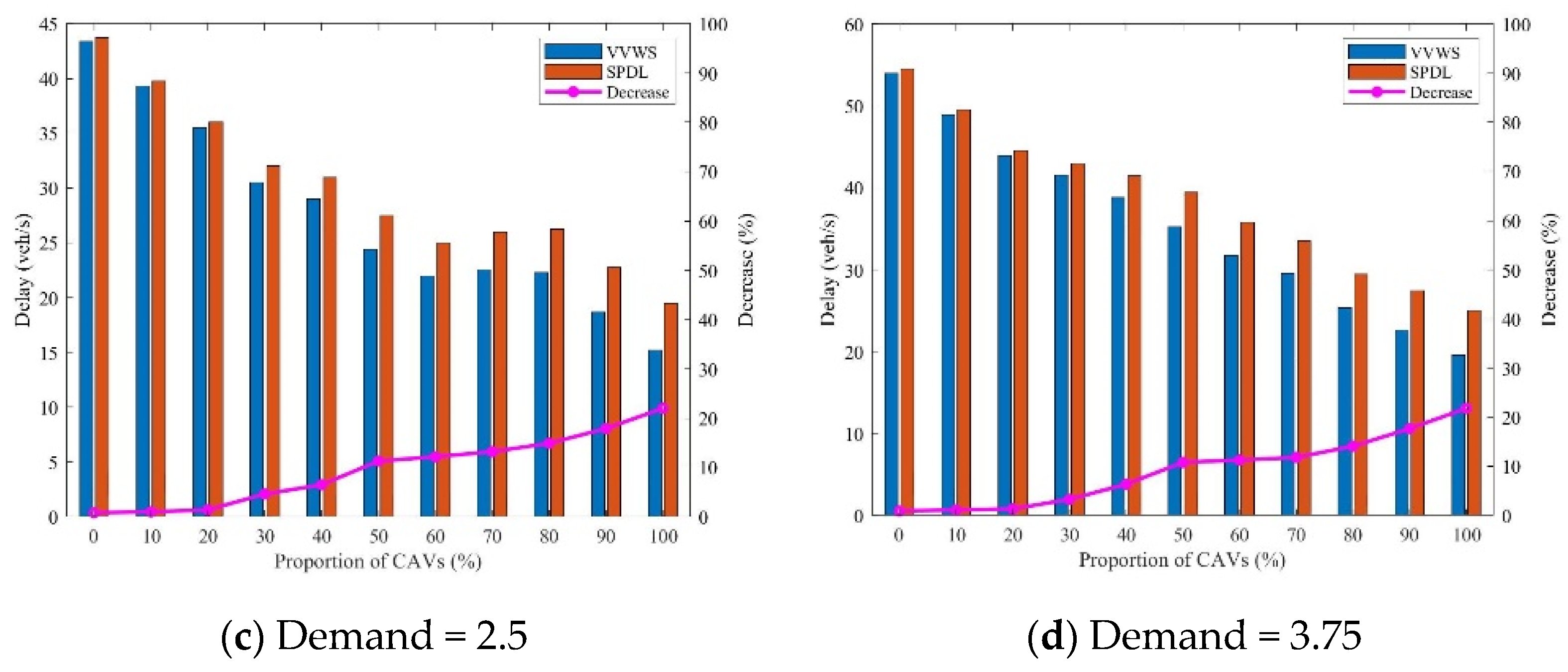
5.3.1. Oversaturation Demand Analysis

To deeply analyse the effect of the VVWL control mode when addressing the problem of oversaturated heterogeneous traffic flow, nine different levels of traffic demand with a progressive relationship are tested in this study, using

Table 1. Fundamental traffic demand.

Traffic Demand in pcu/h
	Left-Turn		Through		Right-Turn
	CAV	HV	CAV	HV
Arm 1	200	200	200	200	100
Arm 2	200	200	200	200	100
Arm 3	200	200	200	200	100
Arm 4	200	200	200	200	100

′s fundamental traffic demand as a foundation, and the demand coefficients range from 0.5 to 4.5 in incremental steps of 0.5. These nine traffic demands contain three categories: unsaturated heterogeneous traffic flow, saturated heterogeneous traffic flow, and oversaturated heterogeneous traffic flow. When the demand coefficient is less than 1.5, the traffic demand is in the unsaturated heterogeneous traffic flow stage; when the demand coefficient is equal to 1.5, the traffic demand is in the saturated heterogeneous traffic flow stage; and when the demand coefficient is greater than 1.5, the traffic demand is in the oversaturated heterogeneous traffic flow stage. Control based on VVWL method is used as the basic control group. The CAV percentage is set to 50% during the simulation.

Figure 17 depicts the trends between the increase in intersection access demand and the average intersection heterogeneous traffic flow vehicle arrivals for both the VVWL-based and SPDL-based control modes. Figure 17a,b show the uniform arrival of vehicles and Poisson arrival of vehicles, respectively. Based on Figure 17 as a whole, when there is an unbalanced demand for transportation flow (there is no demand coefficient bigger than 1.5), the uniform vehicle arrivals and the demand under control based on both VVWL and SPDL are almost identical, which indicates that the intersection can carry the full demand until the junction is fully utilized. When oversaturated traffic flow (demand factor greater than 1.5) occurs, the average intersection volumes under both VVWL-based control and SPDL-based control begin to deviate from the demand curve, while continuing to go higher. This means that some of the phases appear to be unable to keep up with the demand, and some phases are oversaturated with traffic. However, compared to the VVWL control mode, the average number of vehicles under control based on SPDL deviate more from the demand curve. The demand factor is now rising from 1.5 to 3.5, the average capacity of the intersection continues to increase up to the maximum for both control models, and the two average capacity curves become flat. This is because the capacity under both control models reaches the upper limit and cannot cope with the excessive throughput demand. However, it is still evident that the intersection capacity based on VVWL control is consistently greater than the intersection capacity based on SPDL control. After the two average capacity curves become flat (the demand factor is greater than 3.5), the intersection capacity based on VVWL control increases by 6% compared to the average capacity of the intersection based on SPDL control, and the capacity of the dedicated CAV lane (with a variable virtual waiting zone) and HV lane are 10% and 2% more, respectively. The reasons for these changes are the same as those described in 5.2.

The comparison in Figure 18 shows the trend between the increase in intersection access demand and the average intersection heterogeneous traffic flow vehicle delay for both the VVWL-based and SPDL-based control modes. Figure 18a,b shows the uniform arrival of vehicles and Poisson arrival of vehicles, respectively. Figure 18 shows that average vehicle delay across all vehicles under both the VVWL control and the SPDL control increases slightly when there is an unbalanced demand for transportation flow. (There is no demand factor bigger than 1.5.) The typical vehicle delay under VVWS-based control decreases by 13% compared to the average vehicle delay under SPDL-based control, which indicates that the intersection can carry the full demand until the capacity of the intersection is reached, and the vehicle delay is closely related to the intersection control method. When oversaturated traffic flow (demand factor greater than 1.5) occurs, the average vehicle delay at the intersection increases significantly under both VVWL-based and SPDL-based control, with demand factors equal to 1.5 and 4.5; for example, the average vehicle delay increases by 92% and 127% under VVWL-based and SPDL-based control, respectively. This indicates that the average vehicle speed at the intersection decreases as the demand for access increases. However, the typical vehicle delay under control based on VVWL is close to approximately 11% less than the typical vehicle delay under control based on SPDL regardless of the demand factor, which implies that the average intersection vehicle speed under VVWS-based control is greater than the typical intersection vehicle speed under control based on SPDL. The proposed variable virtual waiting zone can effectively reduce the typical intersection vehicle delay, which is consistent with the analysis results in 5.2. To further verify the correctness of this conclusion, Figure 19 investigates the average heterogeneous traffic flow vehicle delay at intersections under different passage demands from both CAV and HV perspectives. With the increase in demand factor, the gap in CAV delay time enhancement under the two control modes is not consistent, and the CAV delay enhancement under control based on VVWL is considerably less than that under SPDL-based control, while the HV delay curves under the two control modes are almost identical. This further confirms that the variable virtual waiting zone can effectively improve the average speed of the CAV fleet and contribute positively to the problem of oversaturated traffic demand at intersections.

5.3.2. Analysis of CAV Permeability under Oversaturation

With an interval step of 10%, the simulation analyses the heterogeneous traffic flow passage delays in ten different processes from 0% to 100% CAV penetration under different control methods. Four traffic demands of 1 veh/s, 2 veh/s, 2.5 veh/s, and 3.75 veh/s are used for comparison. The corresponding demand coefficients of the four traffic demands are 1, 2, 2.5, and 3.75. The results in Figure 20 show that when vehicles arrive with a uniform distribution, the average vehicle delay decreases, with increasing CAV penetration for all four different traffic demands. Overall, increasing the CAV penetration in heterogeneous traffic flows, whether based on the VVWL control approach or the SPDL control approach, is beneficial for reducing vehicle delays. Comparing different traffic demands shows that a typical car delay also improves significantly with the increment of traffic access demand. Unfortunately, regardless of the improvement, a typical car delay under control based on VVWL is significantly lower as opposed to that of under control based on SPDL, and this advantage becomes more obvious the larger the traffic demand is. In Figure 20d, for example, the average vehicle delay decreases as CAV penetration increases under oversaturated traffic demand, and the higher the CAV penetration is, the lower the average vehicle delay control based on VVWL is, in contrast to the under control based on SPDL, with CAV penetrations at 40% and 80%. For example, the reduction in delay is 6.35% and 14.08% for the two control methods, which reflects the advantage of the variable virtual waiting zone in handling oversaturated heterogeneous traffic flows. A similar situation can be seen in Figure 21 for the Poisson vehicle arrival distribution.

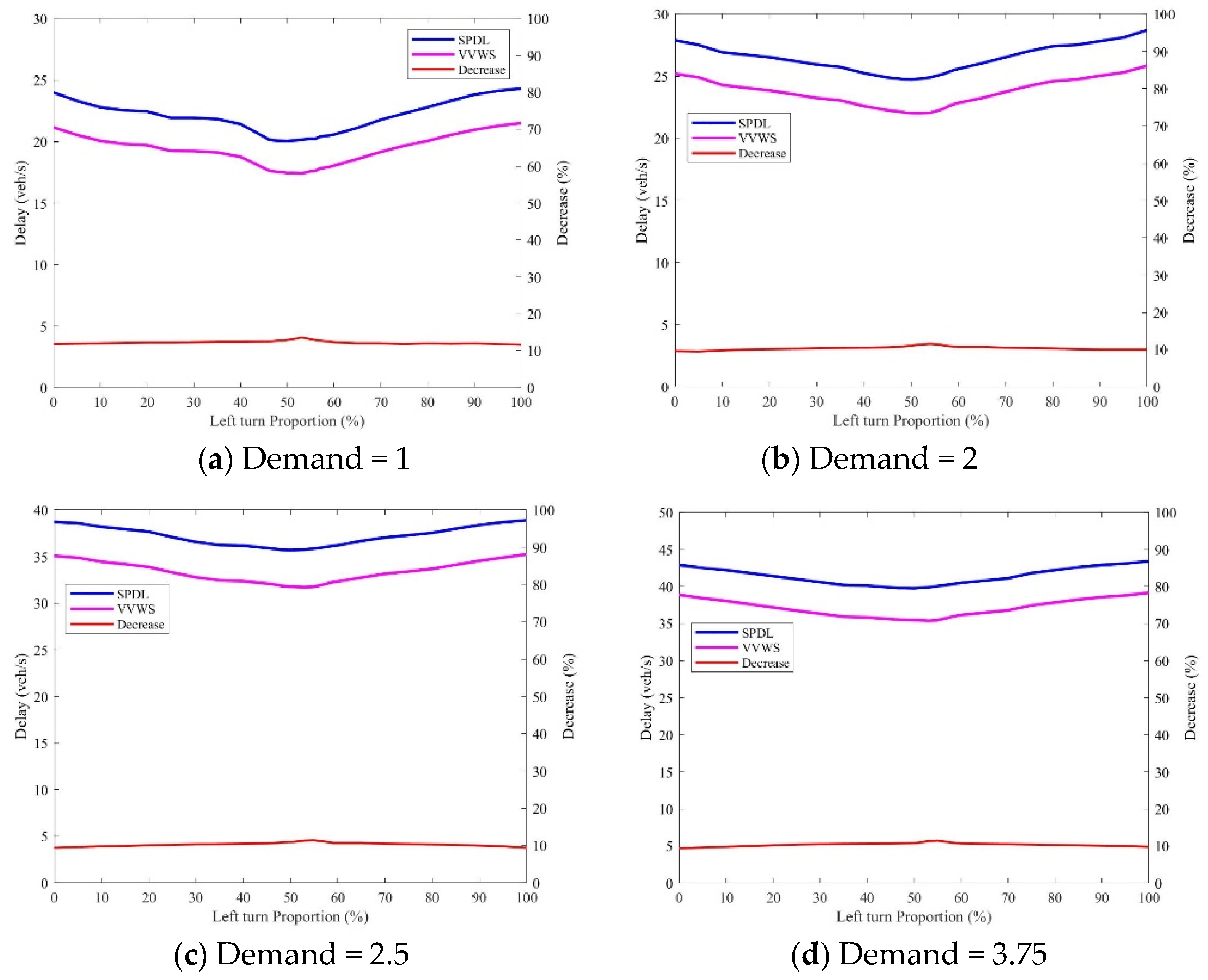
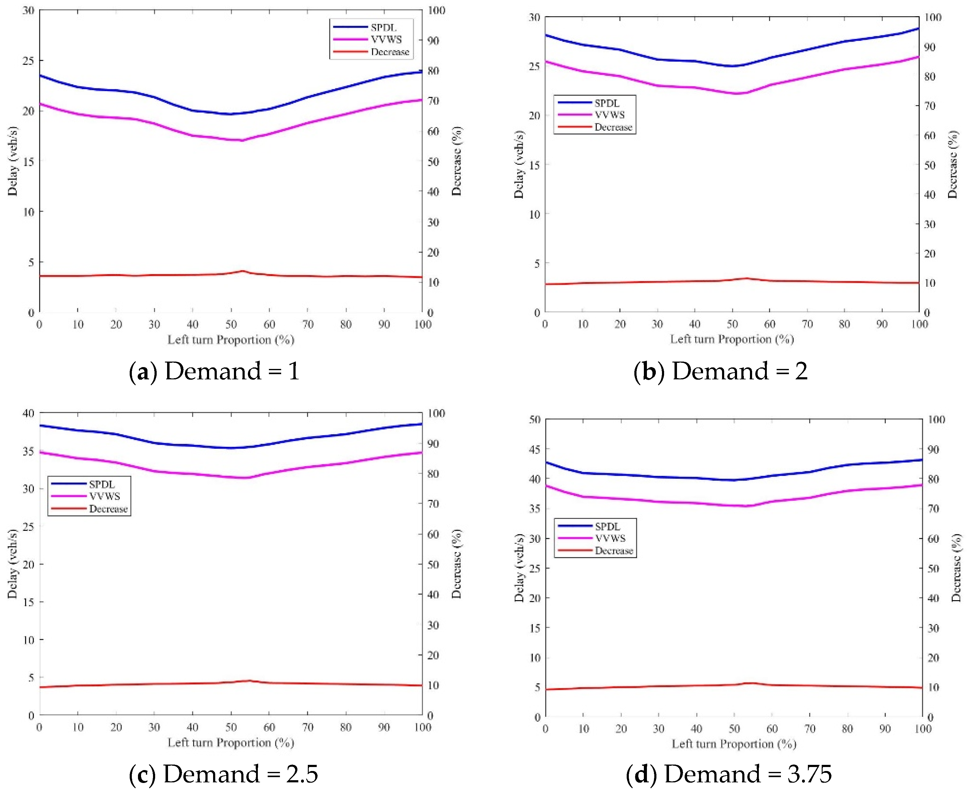
5.3.3. Analysis of CAV Share for Left Turns

In the heterogeneous traffic flow, the CAV percentage is set at 50%. The heterogeneous traffic flow passage delay when the percentage of left-turn CAVs varies from 0% to 100% under different control methods, while considering only straight-ahead and left-turns, is simulated and analysed. Four traffic demands, 1 veh/s, 2 veh/s, 2.5 veh/s and 3.75 veh/s, are used for comparison. The corresponding demand coefficients of the four traffic demands are 1, 2, 2.5, and 3.75. The results in Figure 22 show that the typical vehicle delay under control based on VVWL approach is always less than the typical vehicle delay under control based on VVWL approach, that is, when vehicles are arriving with a uniform distribution for the four different traffic demands. Although the average heterogeneous traffic flow arrival delay under both control methods shows a similar trend with the proportion of left-turning CAVs in the CAV flow rising, that is, it decreases first and then increases, the percentage of left-turning CAVs corresponding to the lowest delay is not the same under both control methods. Under the SPDL-based control approach, the average vehicle delay is minimized only when equal amounts of left-turning and straight-ahead traffic are present, regardless of how the level of traffic has changed. However, the minimum value of the average vehicle delay under VVWL-based control is not fixed at the point where the ratio of through traffic to left-turn traffic is equal, but is slightly greater than 50%. The larger the traffic demand is, the larger the relative value becomes. Taking Figure 22c,d as examples, the left-turn CAV shares corresponding to the minimum average vehicle delay are 55% and 56%, respectively. A further remarkable phenomenon that can be observed is that while travel demand has increased, the lowest point of the typical vehicle delay in the VVWL control mode shifts to the right, while the delay reduction in the control mode based on VVWL becomes increasingly significant compared to the control based on VVWL. The reason for these results is that the overall HV delay is minimized when the ratio of straight-ahead HVs and left-turn HVs is the same. Due to the proposed variable virtual waiting zone, the space resources of the intersection are fully exploited, which makes the CAVs enter the intersection earlier. Given that the size of the left-turn virtual waiting zone is large compared with that of the straight virtual waiting zone, the left-turn CAV running time reduction at the intersection is larger than that of straight CAVs, resulting in a slightly larger number of left-turn CAVs than straight CAVs when the average CAV delay at the intersection is at its minimum, which in turn makes the overall percentage of left-turn CAVs corresponding to the minimum average delay of vehicles slightly larger than 50%. This reflects the advantage of the variable virtual waiting zone in reducing the overall throughput delay and coping with the oversaturated heterogeneous traffic flow. A similar situation is reflected in Figure 23 for the Poisson vehicle arrival distribution.

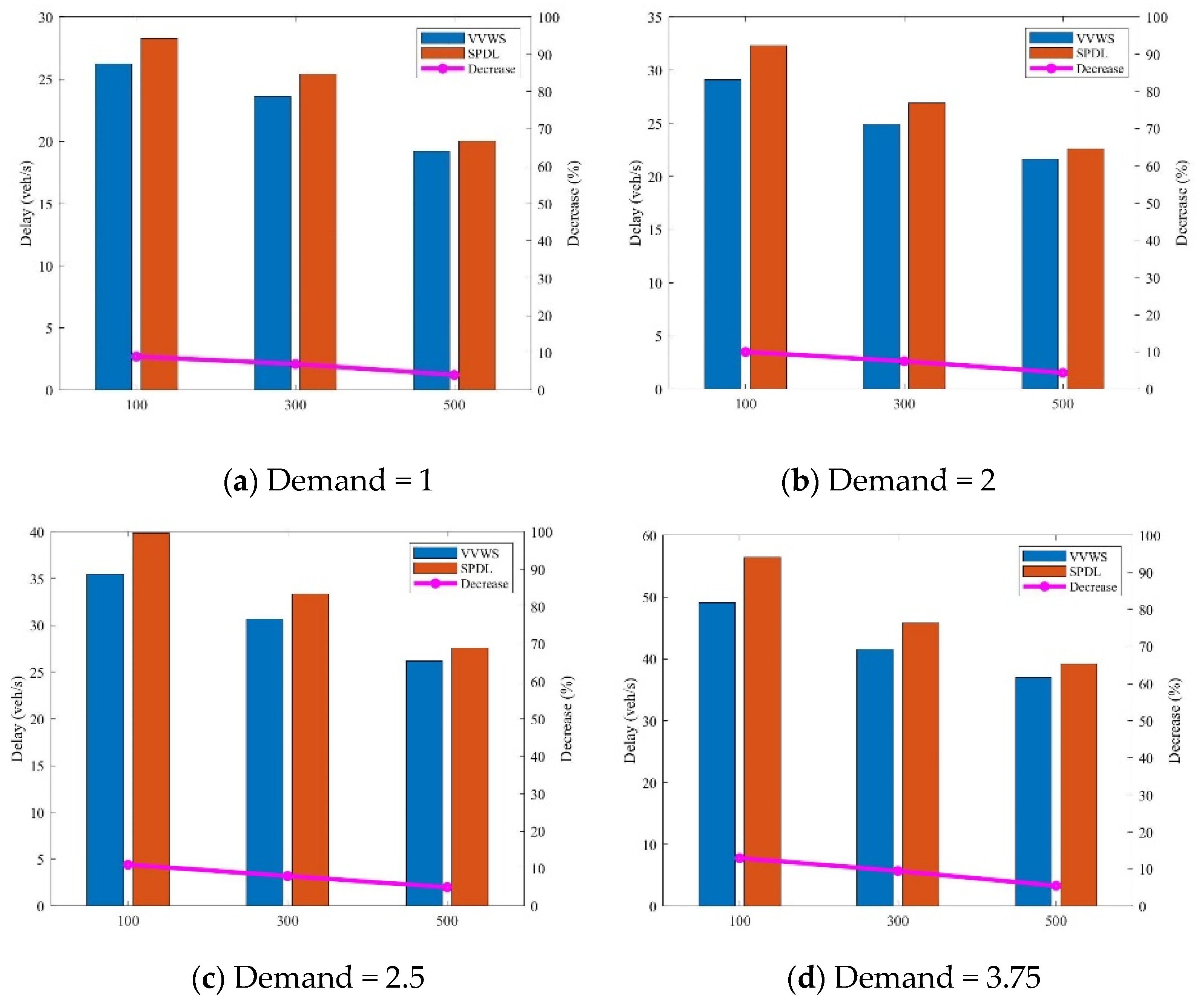
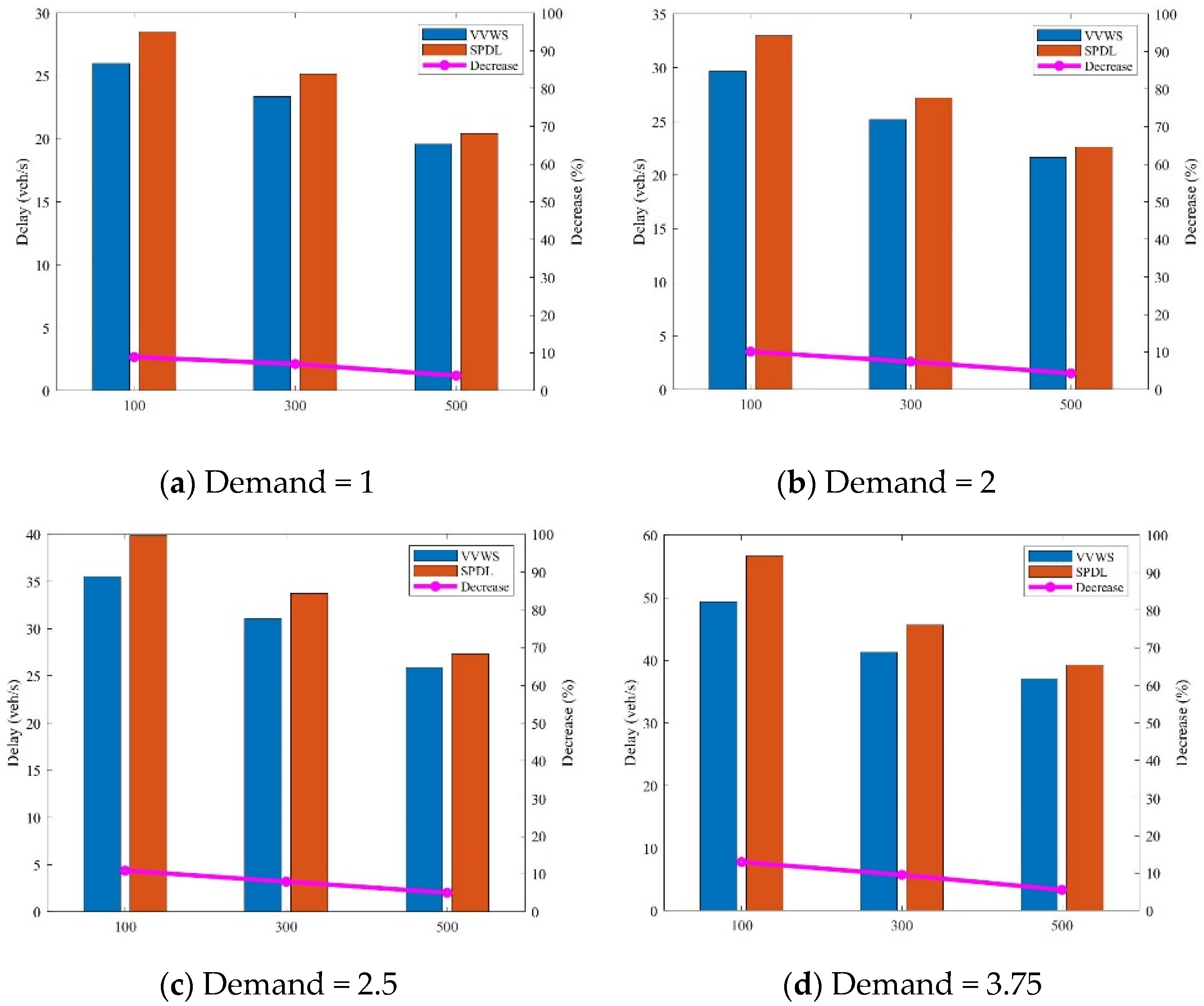
5.3.4. Variable Virtual Waiting Zone Length Analysis

The variable virtual waiting zone makes it possible for CAVs to enter the crossing early during a red light in a nonstop manner, which shortens the CAV passing time. To analyse the effect of variable virtual waiting zone length variation on how well the control model performs, this study sets the size of the left-turn virtual waiting zone and straight virtual waiting zone to 50%, 75%, and 100% of the maximum length under the premise of ensuring traffic safety. The passing zone is 300 m long. Four traffic demands of 1 veh/s, 2 veh/s, 2.5 veh/s, and 3.75 veh/s are used for comparison, and the corresponding demand coefficients of the four traffic demands are 1, 2, 2.5, and 3.75. The comparison in Figure 24 shows the performance difference between the control model based on VVWL and the control model based on SPDL in coping with the variable virtual waiting zone length variation for when the vehicles arrive in an evenly distributed manner with different levels of traffic demand. The variable virtual waiting zone length variation has no effect on the control performance of the control model based on SPDL, and has a greater effect on the control performance of the control model based on VVWL, and the longer the variable virtual waiting zone, the smaller the vehicle delay. Comparing Figure 24a,d, it can be further seen that the higher the pass saturation is, the greater the advantage of the variable virtual waiting zone in reducing vehicle delays. Similar results are obtained in Figure 25 for a Poisson vehicle arrival distribution. There are two reasons for these results: (1) The proposed variable virtual waiting zone allows CAVs to cross the intersection stop line at a relatively high speed. CAV trajectory planning can be delayed inside the variable virtual waiting zone at the intersection, resulting in a relatively high CAV speed in the passing zone, which in turn reduces the delay time. This is shown in Figure 16. (2) The variable virtual waiting zone is equivalent to extending the passing zone of the dedicated CAV lane, providing more space for vehicle speed changes.

6. Conclusions

In this paper, a VVWL-based cooperative control model for oversaturated heterogeneous traffic flow at single intersections is proposed. The model is built on the basis that left-turning CAVs and straight-through CAVs form a CAV dedicated lane, and an overall delay reduction is achieved by tapping the intersection space resources to form a variable virtual waiting zone. A three-layer optimization model with cooperative signal control, vehicle trajectory planning, and variable virtual waiting zone switching is constructed. The upper layer of the model divides the signal control cycle using the standard NEMA ring barrier structure and adopts a rolling time domain scheme to optimize the barrier time. In the middle layer, the phase duration and switching time of the variable virtual waiting zone are optimized based on the fixed phase sequence, and the vehicle delays are returned to the upper optimization model. In the lower layer, CAVs are grouped and the trajectory is planned in the dedicated CAV lane based on signal timing and variable virtual waiting zone durations, and CAV delays are returned to the middle level. Simulations verify that control based on VVWL is significantly better than control based on SPDL in terms of intersection capacity and typical vehicle delay. Sensitivity analysis shows that (1) control based on VVWL is significantly better than control based on SPDL under any traffic demand; (2) control based on VVWL is extremely resistant to CAV penetration; and (3) a longer length of the variable virtual waiting zone is more helpful to the model control.

In this study, only single-intersection access efficiency issues are considered. Passing delays on road segments are not studied in depth. However, the problem of heterogeneous traffic flow on a road segment road network level is worth studying. The optimization of heterogeneous traffic flow on an entire road section and road network in an integrated manner will be a very important research direction.

References

1. Noaeen, M.; Mohajerpoor, R.; Far, B.H.; Ramezani, M. Real-time decentralized traffic signal control for congested urban networks considering queue spillbacks. Transp. Res. C Emerg. Technol. 2021, 113, 103407. [Google Scholar] [CrossRef]
2. Li, Z.; Yu, H.; Zhang, G.; Dong, S.; Xu, C. Network-wide traffic signal control optimization using a multi-agent deep reinforcement learning. Transp. Res. C Emerg. Technol. 2021, 125, 103059. [Google Scholar] [CrossRef]
3. Ren, Y.; Jiang, H.; Ji, N.; Yu, H. TBSM: A traffic burst-sensitive model for short-term prediction under special events. Knowl.-Based Syst. 2022, 240, 108120. [Google Scholar] [CrossRef]
4. Kester, J. Insuring future automobility: A qualitative discussion of British and Dutch car insurer's responses to connected and automated vehicles. Res. Transp. Bus. Manag. 2022, 45, 100903. [Google Scholar] [CrossRef]
5. Zheng, F.; Liu, C.; Liu, X.; Jabari, S.; Lu, l. Analyzing the impact of automated vehicles on uncertainty and stability of the mixed traffic flow. Transp. Res. C Emerg. Technol. 2020, 112, 203–219. [Google Scholar] [CrossRef]
6. Ren, Y.; Jiang, H. Zhang, L.;Liu, R.; Yu, H. HD-RMPC: A Hierarchical Distributed and Robust Model Predictive Control Framework for Urban Traffic Signal Timing. J. Adv. Transp. 2022, 2022, 8131897. [Google Scholar] [CrossRef]
7. Guo, Q.; Ban, X.; Aziz, H. Mixed traffic flow of human driven vehicles and automated vehicles on dynamic transportation networks. Transp. Res. C Emerg. Technol. 2021, 128, 103159. [Google Scholar] [CrossRef]
8. Xu, P.; Li, W.; Hu, X.; Wu, H.; Li, J. Spatiotemporal analysis of urban road congestion during and post COVID-19 pandemic in Shanghai, China. Transp. Res. Interdiscip. Perspect. 2022, 13, 100555. [Google Scholar] [CrossRef] [PubMed]
9. Rosero, F.; Fonseca, N.; López, J.; Casanova, J. Effects of passenger load, road grade, and congestion level on real-world fuel consumption and emissions from compressed natural gas and diesel urban buses. Appl. Energy. 2020, 282, 116–195. [Google Scholar] [CrossRef]
10. Li, Y.; Xiong, W.; Wang, X. Does polycentric and compact development alleviate urban traffic congestion? A case study of 98 Chinese cities. Cities 2019, 88, 100–111. [Google Scholar] [CrossRef]
11. Ma, W.; Li, J.; Yu, C. Shared-phase-dedicated-lane based intersection control with mixed traffic of human-driven vehicles and connected and automated vehicles. Transp. Res. C Emerg. Technol. 2022, 135, 103509. [Google Scholar] [CrossRef]
12. Yang, C.; Chen, X.; Lin, X.; Li, M. Coordinated trajectory planning for lane-changing in the weaving areas of dedicated lanes for connected and automated vehicles. Transp. Res. C: Emerg. Technol. 2022, 144, 103864. [Google Scholar] [CrossRef]
13. Zhao, X.; Gao, Y.; Jin, S.; Xu, Z.; Liu, Z.; Fan, W.; Liu, P. Development of a cyber-physical-system perspective based simulation platform for optimizing connected automated vehicles dedicated lanes. Expert Syst. Appl. 2022, 213, 118972. [Google Scholar] [CrossRef]
14. Ye, L.; Yamamoto, T. Impact of dedicated lanes for connected and autonomous vehicle on traffic flow throughput. Phys. A Stat. Mech. Its Appl. 2018, 512, 588–597. [Google Scholar] [CrossRef]
15. Jiang, Z.; Yu, D.; Luan, S.; Zhou, H.; Meng, F. Integrating traffic signal optimization with vehicle microscopic control to reduce energy consumption in a connected and automated vehicles environment. J. Clean. Prod. 2022, 371, 133694. [Google Scholar] [CrossRef]
16. Datesh, J.; Scherer, W.T.; Smith, B.L. Using K-Means Clustering to Improve Traffic Signal Efficacy in an IntelliDrive SM Environment. In Proceedings of the IEEE Forum on Integrated and Sustainable Transportation Systems, Vienna, Austria, 29 June–1 July 2011; pp. 122–127. [Google Scholar]
17. Feng, Y.; Head, K.L.; Khoshmagham, S.; Zamanipour, M. A real-time adaptive signal control in a connected vehicle environment. Transp. Res. C Emerg. Technol. 2015, 55, 460–473. [Google Scholar] [CrossRef]
18. Shaghaghi, E.; Jabbarpour, M.R.; Md Noor, R.; Yeo, H.; Jung, J.J. Adaptive green traffic signal controlling using vehicular communication. Frontiers of Information Technol. Electron. Eng. 2017, 18, 373–393. [Google Scholar] [CrossRef]
19. Rey, D.; Levin, M.W. Blue phase: Optimal network traffic control for legacy and autonomous vehicles. Transp. Res. B Methodol. 2019, 130, 105–129. [Google Scholar] [CrossRef] [Green Version]
20. Liang, X.; Guler, S.; Gayah, V. Decentralized arterial traffic signal optimization with connected vehicle information. J. Intell. Transp. Syst. 2021, 27, 1990762. [Google Scholar] [CrossRef]
21. Islam, S.; Hajbabaie, A.; Aziz, H. A real-time network-level traffic signal control methodology with partial connected vehicle information. Transp. Res. C Emerg. Technol. 2020, 121, 102830. [Google Scholar] [CrossRef]
22. Yao, Z.; Zhao, B.; Yuan, T.; Jiang, H.; Jiang, Y. Reducing gasoline consumption in mixed connected automated vehicles environment: A joint optimization framework for traffic signals and vehicle trajectory. J. Clean. Prod. 2020, 265, 121836. [Google Scholar] [CrossRef]
23. Zhang, L.; Yuan, Z.; Yang, L.; Liu, Z. Recent developments in traffic flow modeling using macroscopic fundamental diagram. Transp. Rev. 2020, 40, 529–550. [Google Scholar] [CrossRef]
24. Kamal, M.; Imura, J.; Hayakawa, T.; Ohata, A.; Aihara, K. Traffic Signal Control in an MPC Framework Using Mixed Integer Programming. IFAC Proc. Vol. 2013, 46, 645–650. [Google Scholar] [CrossRef]
25. Park, B.; Yun, I.; Ahn, K. Stochastic optimization for sustainable traffic signal control. Int. J. Sustain. Transp. 2009, 4, 263–284. [Google Scholar] [CrossRef]
26. Wang, S.; Ahmed, N.; Yeap, T. Optimum Management of Urban Traffic Flow Based on a Stochastic Dynamic Model. IEEE Trans. Intell. Transp. Syst. 2019, 12, 4377–4389. [Google Scholar] [CrossRef]
27. Huang, W.; Li, L.; Lo, H. Adaptive traffic signal control with equilibrium constraints under stochastic demand. Transp. Res. C Emerg. Technol. 2018, 95, 394–413. [Google Scholar] [CrossRef]
28. Yan, Y.; Qu, X.; Li, H. On the design and operational performance of waiting areas in at-grade signalized intersections: An overview. Transp. A Transp. Sci. 2018, 14, 901–928. [Google Scholar] [CrossRef]
29. Ren, Y.; Jiang, H.; Feng, X.; Zhao, Y.; Liu, R.; Yu, H. ACP-Based Modeling of the Parallel Vehicular crowd sensing system: Framework, components and an application example. IEEE Trans. Intell. Veh. 2022, 3221927. [Google Scholar] [CrossRef]
30. Yang, Q.; Shi, Z. Effects of the design of waiting areas on the dynamic behavior of queues at signalized intersections. Phys. A Stat. Mech. Its Appl. 2018, 509, 181–195. [Google Scholar] [CrossRef]
31. Yang, Z.; Liu, P.; Tian, Z.; Wang, W. Effects of left-turn waiting areas on capacity and level of service of signalized intersections. J. Transp. Eng. 2013, 139, 1076–1085. [Google Scholar] [CrossRef]
32. Ma, W.; Liu, Y.; Zhao, J.; Wu, N. Increasing the capacity of signalized intersections with left-turn waiting areas. Transp. Res. A. 2017, 105, 181–196. [Google Scholar] [CrossRef]
33. Jiang, X.; Zhang, G.; Zhou, Y.; Xia, L.; He, Z. Safety assessment of signalized intersections with through-movement waiting area in China. Saf. Sci. 2017, 95, 28–37. [Google Scholar] [CrossRef]
34. Jiang, X.; Zhang, G.; Bai, W.; Fan, W. Safety evaluation of signalized intersections with left-turn waiting area in China. Accid. Anal. Prev. 2016, 95, 461–469. [Google Scholar] [CrossRef] [Green Version]
35. Qin, Z.; Shao, H.; Wang, F.; Feng, Y.; Shen, L. A reliable energy consumption path finding algorithm for electric vehicles considering the correlated link travel speeds and waiting times at signalized intersections. Sustain. Energy Grids Netw. 2022, 32, 100877. [Google Scholar] [CrossRef]
36. Amouzadi, M.; Orisatoki, M.; Dizqah, A. Lane-free crossing of cavs through intersections as a minimum-time optimal control problem. IFAC-PapersOnLine 2022, 55, 28–33. [Google Scholar] [CrossRef]
37. Rad, S.; Farah, H.; Taale, H.; Arem, B.; Hoogendoorn, S. Design and operation of dedicated lanes for connected and automated vehicles on motorways: A conceptual framework and research agenda. Transp. Res. C Emerg. Technol. 2020, 117, 102664. [Google Scholar]
38. Chalaki, B.; Malikopoulos, A.A. Optimal control of connected and automated vehicles at multiple adjacent intersections. IEEE Trans. Control. Syst. Technol. 2021, 3, 972–984. [Google Scholar] [CrossRef]
39. Yu, C.; Sun, W.; Liu, H.X.; Yang, X. Managing connected and automated vehicles at isolated intersections: From reservation to optimization-based methods. Transp. Res. Part B Methodol. 2019, 122, 416–435. [Google Scholar] [CrossRef]
40. Tajeddin, S.; Ekhtiari, S.; Faieghi, M.; Azad, N.L. Ecological adaptive Cruise control with optimal lane selection in connected vehicle environments. IEEE Trans. Intell. Transp. Syst. 2020, 21, 4538–4549. [Google Scholar] [CrossRef]
41. Li, M.; Wu, X.; He, X.; Yu, G.; Wang, Y. An eco-driving system for electric vehicles with signal control under V2X environment. Transp. Res. C Emerg. Technol. 2018, 93, 335–350. [Google Scholar] [CrossRef]
42. Zhao, W.; Ngoduy, D.; Shepherd, S.; Liu, R.; Papageorgiou, M. A platoon based cooperative eco-driving model for mixed automated and human-driven vehicles at a signalised intersection. Transp. Res. C Emerg. Technol. 2018, 95, 802–821. [Google Scholar] [CrossRef] [Green Version]
43. Malikopoulos, A.; Cassandras, C.; Zhang, Y. A decentralized energy-optimal control framework for connected automated vehicles at signal-free intersections. Automatica 2018, 93, 244–256. [Google Scholar] [CrossRef] [Green Version]
44. Ma, C.; Yu, C.; Yang, X. Trajectory planning for connected and automated vehicles at isolated signalized intersections under mixed traffic environment. Transp. Res. C Emerg. Technol. 2021, 130, 103309. [Google Scholar] [CrossRef]
45. Wan, N.; Vahidi, A.; Luckow, A. Optimal speed advisory for connected vehicles in arterial roads and the impact on mixed traffic. Transp. Res. C Emerg. Technol. 2016, 69, 548–563. [Google Scholar] [CrossRef]
46. Feng, Y.; Yu, C.; Liu, H. Spatiotemporal intersection control in a connected and automated vehicle environment. Transp. Res. C Emerg. Technol. 2018, 89, 364–383. [Google Scholar] [CrossRef]
Figure 1. Typical heterogeneous signal intersections with dedicated CAV lanes and variable virtual waiting zones.
Applsci 13 03054 g001
Figure 2. Intersection lane group division.
Applsci 13 03054 g002
Figure 3. Variable virtual waiting zone and associated signal phase. (a). Passage trajectory and virtual variable waiting zone. (b). Intersection signal phase. (c). Passage trajectory and virtual. (d). Intersection signal phase.
Applsci 13 03054 g003
Figure 4. Three-layer optimization model framework.
Applsci 13 03054 g004
Figure 5. Ring barrier controller structure.
Applsci 13 03054 g005
Figure 6. Dynamic planning variables.
Applsci 13 03054 g006
Figure 7. Rolling repeated barrier group scheme.
Applsci 13 03054 g007
Figure 8. Forwards recursion flow chart.
Applsci 13 03054 g008
Figure 9. Backwards recursion flow chart.
Applsci 13 03054 g009
Figure 10. CAV trajectory queue. (a) Case 1 utilizing two platoons. (b) Case 2 utilizing one platoon.
Applsci 13 03054 g010aApplsci 13 03054 g010b
Figure 11. Acceleration profile.
Applsci 13 03054 g011
Figure 12. Two illustrative paths with the same travel distance.
Applsci 13 03054 g012
Figure 13. Two demonstrative trajectories with the same travel time.
Applsci 13 03054 g013
Figure 14. Vehicle passage. (a) Uniform arrival of vehicles; b) Poisson arrival of vehicles.
Applsci 13 03054 g014
Figure 15. Average vehicle delay. (a) Uniform arrival of vehicles; (b) Poisson arrival of vehicles.
Applsci 13 03054 g015
Figure 16. CAV intersection speed analysis.
Applsci 13 03054 g016
Figure 17. Flow of vehicles (veh/h). (a) Uniform arrival of vehicles; (b) Poisson arrival of vehicles.
Applsci 13 03054 g017
Figure 18. Average vehicle delay across all vehicles. (a) Uniform arrival of vehicles; (b) Poisson arrival of vehicles.
Applsci 13 03054 g018
Figure 19. CAV and HV delays on average. (a) Uniform arrival of vehicles; (b) Poisson arrival of vehicles.
Applsci 13 03054 g019
Figure 20. Effects of CAV penetration rates on vehicle delay when the distribution of vehicle arrivals is uniform.
Applsci 13 03054 g020
Figure 21. Effects of CAV penetration rates on vehicle delay when the distribution of vehicle arrivals is Poisson.
Applsci 13 03054 g021aApplsci 13 03054 g021b
Figure 22. Effect of left-turn proportions on vehicle delay when the distribution of vehicle arrivals is uniform.
Applsci 13 03054 g022
Figure 23. Effect of left-turn proportions on vehicle delay when the distribution of vehicle arrivals is Poisson.
Applsci 13 03054 g023
Figure 24. A uniform distribution of vehicles arriving on time and the effect of a varied virtual waiting zone duration on vehicle delay.
Applsci 13 03054 g024
Figure 25. A Poisson distribution of vehicles arriving on time and the effect of a varied virtual waiting zone duration on vehicle delay.
Applsci 13 03054 g025