Article

Study of Applicability of Triangular Impulse Response Function for Ultimate Strength of LNG Cargo Containment Systems under Sloshing Impact Loads

Department of Naval Architecture and Offshore Engineering, Dong-A University, Busan 49315, Republic of Korea
*
Author to whom correspondence should be addressed.
Appl. Sci. 2023, 13(5), 2883; https://doi.org/10.3390/app13052883
Submission received: 6 December 2022 / Revised: 17 February 2023 / Accepted: 20 February 2023 / Published: 23 February 2023
(This article belongs to the Special Issue Ship Structures: Design Loads and Reliability Assessment)

Abstract

:
The LNG cargo containment system used in membrane-type LNG cargo tanks must have sufficient dynamic strength to withstand the impact of sloshing loads. However, performing direct dynamic nonlinear transient finite element assessments against design sloshing impact loads with different design specifications can be complicated and time-consuming. To address this, it is effective to use linear superposition methods, such as the triangular impulse response function (TIRF) method, to conduct dynamic transient FE assessments of LNG cargo containment systems. However, as LNG cargo containment systems have a high level of nonlinearities in terms of geometry, material, and boundary effects, it is necessary to evaluate the applicability of the TIRF method in advance. This study investigates the dynamic responses of an LNG cargo containment system using the TIRF method and compares the ultimate value of the structural responses and impulses with that obtained using direct dynamic nonlinear transient assessments. Based on a comparison of a series of FE analyses, the study proposes a design for the partial safety factors for calculating the ultimate bending and shear capacities of an LNG cargo containment system, taking into consideration the dynamic impact of sloshing loads using the TIRF method. Finally, the ultimate shear and bending capacities are calculated using the proposed method and compared with those obtained through direct dynamic nonlinear transient assessments. The results show that the proposed method provides conservative estimates against direct nonlinear finite element simulations, with a difference of around 10% for the mean minus two standard deviations. This approach can be practically applied for early basic design purposes in the shipbuilding industry.

1. Introduction

Owing to the International Maritime Organization’s (IMO) environmental regulations, the demand for clean energy has increased significantly, particularly for decarbonization. Although hydrogen and ammonia-fueled vessels are still in the early stages of development, the demand for conventional liquified natural gas (LNG) as an energy resource is on the rise.
The membrane-type LNG cargo tank is the most popular LNG containment system due to its cargo transportation efficiency. The most critical factor in the design of an LNG cargo containment system (CCS) is securing enough dynamic strength against the sloshing impact load [1].
To evaluate the strength of a CCS against the sloshing load, it is necessary to calculate the pressure from a hydrodynamic point of view and to evaluate the structural strength in various failure modes, i.e., crushing, shear, bending, and buckling, for the impact pressure. Experiments and numerical analyses are mainly performed to estimate the sloshing pressure. Lu et al. [2] carried out a series of sloshing experiments to investigate fluid sloshing for different filling levels in a rectangular tank. Xue et al. [3] studied the effectiveness of the four types of baffles in suppressing the pressure for a wide range of forcing frequencies. Zhang et al. [4] carried out a series of experiments on the hydrodynamics of an anti-sloshing technique using floating foams in a rectangular liquid tank, and an analytical potential flow solution was derived to explain the experimental observations. The effects of the various layers of floating foams on both the wave profiles and dynamic pressure histories in sloshing tanks were analyzed. Ahn et al. [5] developed sloshing load prediction using the artificial neural network method with an experimental database from the model scaled sloshing test. Pilloton et al. [6] carried out a numerical investigation of sloshing flows inside the LNG fuel tank of a ship using the smoothed particle hydrodynamics model (SPH). Xue et al. [7] performed computational fluid dynamics (CFD) calculations to study the sloshing wave interaction with the porous material layer. The improved model used to simulate the porous breakwater was validated against the available experimental data. Ding et al. [8] focused on the sloshing simulation of an ice-breaking LNG carrier and proposed a numerical method using the circumferential crack method (CCM) and volume of fluid (VOF) with two key factors. Tang et al. [9] compared the influence of different baffle factors, such as the number of baffles, liquid rate, and excitation frequency, through CFD simulations. Then, they compared the sloshing characteristics for those parameters by investigating the wave height, spectrum, hydrodynamic force, and velocity vector.
However, owing to the randomness of the sloshing phenomenon, it is difficult to standardize the sloshing pressure applicable to the design stage. It is common practice to apply the impact pressure in a simplified form in the form of a triangle with a specific peak pressure and rise time [10,11]. The peak pressure and rise time are normally determined based on the statistical data obtained through experiments and measurements.
Although the simplified load history is applied, when it is applied to the structure, caution is still required due to the strong nonlinearity of the structure, the LNG box. This is because, in the case of the NO96-type CCS, a containment system consisting of complex parts, such as tongue, membrane, and weld joints (Figure 3 Schematic of the structural boundary nonlinearity in LNG CCS application(a)), is applied to prevent heat shrinkage/expansion/heat conduction at cryogenic temperatures. Therefore, as the complexity of the strength evaluation for sloshing is very high in terms of the hydrodynamic pressure and structural response, it is recommended that one considers the effects of all the possible factors in a complex way in the calculation, which is time consuming.
Several studies have been conducted on the efficient evaluation of sloshing strength under a given sloshing pressure. Kim and Kim [12] proposed a strength assessment procedure based on the convolution integral method using the triangular impulse function (TIRF). They applied the TIRF to obtain the dynamic response of the LNG CCS and performed a statistical analysis of the peak stress. Kim [13] performed a rapid response calculation of the LNG CCS under sloshing impact using the wavelet transformation technique. He decomposed the sloshing pressure history obtained from the model test into the wavelet basis function and ensured an efficient calculation of the response by combining these results with the structural analysis results. Nho et al. [14] applied the TIRF to evaluate the strength of the Mark-III cargo containment system. They examined how the system’s structure reacted when exposed to a specific pattern of sloshing impact pressure over time that was obtained from a small-scale model test.
There have been several studies investigating the use of TIRF approaches for dynamic transient simulation purposes. However, it should be noted that the TIRF approach is theoretically applicable only to linear systems, such as steel structures. In contrast, the current study focuses on nonlinear systems, including nonlinear geometry, nonlinear material properties, and nonlinear boundary conditions, to evaluate whether a linear-based TIRF method can be used for the structural evaluation of an LNG CCS that consists of layered composite materials and complex boundary conditions.
The aim of this study is to develop design guidelines that can evaluate the dynamic impact structural response of the NO96-type LNG CCS against the sloshing impact load easily and effectively. Considering the various nonlinear factors of geometry, material, and boundary conditions, the applicability of the TIRF-based linear superposition method was evaluated and compared to the time-consuming Direct (DIR) method. We tried to apply the TIRF method to models with various boundary conditions and nonlinearities for practical applications, and quantitatively evaluated it to derive a partial factor that can be applied to the actual design. Finally, the actual ultimate strength was evaluated based on the proposed guideline and compared with that of the DIR method.

2. Failure Modes of NO96-Type LNG CCS

DNVGL-CG-0158 [15] defines the following four typical failure modes for NO96-type LNG CCSs:
(1)
A shear failure of the cover plate of the primary box;
(2)
A sending failure of the cover plate of the primary box;
(3)
A crushing failure of the plates at the bulkhead intersections;
(4)
A buckling failure of the primary and the secondary bulkhead plates.
DNVGL-CG-0158 [15] provides the design formula to calculate the ultimate shear, bending, crushing, and buckling strength against the sloshing impact pressure as Equations (1)–(3).
Equations (1) and (2) are the design criteria to calculate the ultimate dynamic shear and bending capacities. The reference dynamic shear and bending stresses per unit of pressure can be obtained through time domain dynamic transient numerical simulations, depending on the various rise times of the dynamic impact profiles and load areas. Then, the reference dynamic shear and bending stresses are linearly multiplied until the dynamic stresses reach the design shear and bending values, as listed in Table 1.
A large number of time domain DIRs must be carried out to cover all the possible ultimate dynamic shear and bending capacities depending on the sloshing impact load profiles. Therefore, a series of FE assessments based on the TIRF approach and the DIR were carried out to determine the ultimate shear and bending capacities, and the applicability of the TIRF approach to the LNG cargo containment system was reviewed.
Q D A F Q c
M D A F M c
where Q = the calculated section shear force per unit of plate width at the highest loaded cross section of the cover plate of the primary box; Q c = the section shear force capacity of the cover plate of the primary box for the considered material’s orientation; M = the calculated bending moment per unit of plate width at the highest loaded cross section of the cover plate of the primary box; M c = the bending moment capacity of the plywood plate; and D A F = the dynamic amplification factor of design load.
The crushing strength check should be carried out using the following:
σ a v D A F γ F σ c a v γ M
where σ a v = the nominal stress in the bulkhead plates of the primary box in the region of the bulkhead intersections; σ c a v = the through-thickness compressive strength of the plywood plate measured in terms of the nominal stress in the secondary box bulkhead; and γ F , γ M = the partial load and material factors, respectively.
The crushing failure assessment should be determined through the thickness material criteria of the plywood panels.
In this study, the shell element was used for the basic FE model of the LNG cargo containment boxes, and because the shell element is limited in the stress evaluation in the through-thickness direction of the elements, crushing assessments are excluded from this study.
Equation (4) shows the design’s dynamic ultimate buckling strength for the LNG cargo containment system. The equation consists of the dynamic amplification factor (DAF) and dynamic buckling strength criteria as a function of the slenderness ratio in Equation (5).
To calculate the dynamic ultimate buckling strength, the linear static buckling strength of the plywood box incorporates the anisotropic elastic modulus of the plywood panels depending on the loading types, i.e., the membrane force and bending force. The reference compressive stress of the plywood box per unit of pressure can be calculated through numerical simulations depending on the load areas and other environmental conditions, such as temperature. Then, the calculated reference stress value is linearly multiplied until the limited value is reached to obtain the ultimate static buckling capacities using Equation (5).
The ultimate static buckling strength needs to be multiplied by the dynamic strength factor (DSF), as shown in Equation (6), to obtain the ultimate dynamic buckling strength of the plywood box.
The ultimate dynamic buckling capacities depending on the load areas, various dynamic impact load profiles, and other environmental conditions, can be easily calculated as described earlier by considering the DSF without the DIR for complicated design parameters. Therefore, in this study, buckling dynamic strength calculations are not considered.
σ D A F σ c D
where σ c D = the dynamic buckling strength of the plywood panels; and D A F = the dynamic amplification factor.
σ c σ F = 1.05 + λ 2 ( 1.05 + λ 2 ) 2 4 λ 2 2 λ 2
where
λ = σ F σ E = the   slenderness   ratio σ c = the   designs s   static   buckling   strength σ E = k 1 σ E , 1 + k 2 σ F σ E , 1 = π 2 D 12 ( t h ) 2 D = h 4 { E b , 1 h 4 + E b , 2 B 4 + 2 h 2 B 2 ( ν 12 E b , 2 + 2 G 12 ) }
σ E , 1 = the elastic buckling stress for a simply supported bulkhead subjected to uniform load.
σ F = the plywood material compressive strength; E b , 1 = the plywood bending modulus in the strong direction; E b , 2 = the plywood bending modulus in the weak direction; h = the plywood height; B = the plywood breadth; ν 12 = the Possion’s ratio; G 12 = the shear modulus; k 1 = the factor depending on the size of the load-exposed region of the bulkhead; k 2 = the factor to account for the increased buckling strength of slender bulkheads caused by the rotational restraint resulting from the finite thickness of the bulkheads.
σ c D = σ c D S F
where
D S F = { f 1 ( λ ) f 1 ( λ ) f 2 ( λ ) 0.55 t r T e f o r t r T e 0.55 f 2 ( λ ) ( f 2 ( λ ) 1 0.95 ) ( t r T e 0.55 ) f o r 0.55 < t r T e 1.50 1.0 f o r t r T e > 1.50
f 1 ( λ ) = f 3 σ F σ c , max . = 4 f 3 = 0.95 f 2 = min ( f 1 ( λ ) , 1.5 )

3. Triangular Impulse Response Function (TIRF)

The sloshing impact load in the membrane-type LNG tank due to the motion of the ship should be a typical irregular impact load with various rise times/impact peak loads/duration times. The corresponding dynamic structural responses are also complicated. Moreover, a time-consuming process is required to deal with the enormous amount of pressure data from the model test and/or simulation results depending on the size of the LNG cargo tank and design environmental conditions. Therefore, the linear superposition approach could be applied to evaluate the dynamic structural assessment for computational efficiency [8,9,14].
In a linear and time-invariant system, its response y ( t ) for any input x ( t ) can be expressed by an impulse response function (IRF) based on a convolution equation as follows:
y ( t ) = x ( t ) × h ( t ) = + x ( t ) h ( t τ ) d τ
where h ( t ) is the impulse response of the system at the origin in time. When the convolution equation in Equation (7) is applied to the LNG cargo containment system, y ( t ) is the response of the box, i.e., the stress component, force, moment, and displacement at critical locations; x ( t ) represents the sloshing load acting on the box; and h ( t ) is the dynamic response calculated at the critical location when a unit impulse is applied to the box.
Kim and Kim and Noh et al. [8,14] applied a discrete form of an IRF with a triangular impulse response to calculate the efficiency. The TIRF can be defined as the time history of the structural response to a symmetric triangular impulse with a short duration, from which triangular impulses with durations and rise times that are integer multiples of the short duration can be generated. Equation (8) is the discrete form with the TIRF of Equation (7).
y ( t ) = i = 1 n x i H i ( t )
S i ( t ) = [ 1 Δ t ( t t i 1 ) f o r t i 1 t < t i 1 1 Δ t ( t t i ) f o r t i t < t i + 1 0 e l s e w h e r e
where x i is the sloshing load at t = t i H i ( t ) is the TIRF for the unit triangular impulse S i ( t ) in Equation (9) and Figure 1. Δ t is the size of the time increment. The calculation process for Equation (8) is described in Figure 2.

4. FE Model Nonlinearities

According to the conventional FE assessment, there could be three nonlinearities for the FE modeling scheme, which are as follows: (1) geometrical nonlinearity, (2) material nonlinearity, and (3) boundary nonlinearity.
As the TIRF is based on the linear superposition method, a series assessment for the effect of the nonlinearities on the ultimate strength assessments is required. However, the effect of material nonlinearity is excluded from this study as the major strength member of the NO96-type LNG cargo containment system is a typical brittle material.
A box-type LNG cargo containment system (GTT NO96) consists of the primary box and the secondary box, which are connected through an elastic coupler system. Therefore, the boundary conditions between the bottom of the primary box and the top of the secondary box are in surface-to-surface contact, similar to the typical nonlinear boundary condition (A in Figure 3a). In addition, there are discontinued panels in the top plate of the primary box owing to the tongue (B in Figure 3a) and primary membrane connection purpose, as shown in Figure 3.
Furthermore, the nonlinear boundary effect between the bottom of the LNG cargo containment system and hull part was studied (C in Figure 3b).

5. FE Models

The TIRF method applied in this study is more efficient than the DIR as it uses a linear superposition method. However, it has a limitation as it can be used only under a linear system. As explained in the previous section, strictly speaking, TIRFs cannot be used in LNG systems because there are distinct non-linearities, such as geometry and boundary conditions.
As computational efficiency is the first priority from the point of view of design applications, this study investigates whether the TIRF method can be used despite such nonlinearity. We intend to quantitatively examine the degree of error, which occurs when this method is applied to a nonlinear system, and to present a guideline that can be applied to the design.
In this study, three models were investigated, as listed in Table 2. As the model number increases, i.e., from Model 1 to Model 3, the complexity and nonlinearity of the overall model increase. For all the models, geometric nonlinearity based on the large deflection theory was considered, and linear and nonlinear boundary conditions were applied, respectively. In all cases, the results derived by the method using the TIRF and the results derived through the DIR were compared. In Model 1, a simple uniform pressure was applied to the top of the model (Figure 4), while in Model 2 and Model 3, all 12 sloshing load conditions, as shown in Figure 5, were considered. Figure 5 shows the typical load-exposed areas, which can be divided into 24 areas [1]. This study selected 12 load areas considering geometrical symmetricity. For each case, five rise times, which were selected according to the study by Park and Kim [1], were applied to consider the dynamic effect.
The primary purpose of Model 1 was to confirm the feasibility of the dynamic structural responses using the TIRF method based on the linear superposition method. Therefore, two simple steel boxes were stacked on top of each other with linear and nonlinear boundary conditions, respectively. Material nonlinearity was excluded, and the element size of the FE model was approximately 24 mm × 24 mm, which was determined based on the results of a mesh sensitivity study conducted by Park and Kim [1].
The purpose of Model 2 was to verify the TIRF method to calculate the ultimate dynamic strength of the LNG boxes against LNG sloshing pressure. As shown in Figure 3a, the secondary box and the primary box were connected by the surface-to-surface contact condition, and the simply supported boundary condition was applied to the bottom surface of the model to avoid the effect of hull deformation. Material nonlinearity was not considered as the strength member of Model 2; i.e., plywood is a typical brittle material and the nickel 36% membrane is excluded. A homogeneous linear orthotropic elastic material was applied to the plywood panels. The dimensions of the average FE model for the LNG cargo containment system were approximately 22 mm × 22 mm.
Model 3 includes the hull steel structure in Model 2 to consider the LNG carrier onboard boundary condition. Similar to Model 2, the FE model was applied to the LNG cargo containment boxes, and FE elements with dimensions of 60 mm × 60 mm were considered for the hull structure. The boundary conditions for the hull structure in Model 3 are shown in Figure 6.
The commercial FE program Abaqus/Explicit was employed for the transient dynamic analysis; the four-node shell element with reduced integration was used. The material properties of the plywood panels are listed in Table 3.
The TIRF’s applicability in the dynamic structural assessment was confirmed by comparing the magnitude of the stress peak values and impulse values, as shown in Figure 7, for the time histories by the TIRF and DIR, respectively.

6. Result of Case Studies

In this section, the analysis results for the cases listed in Table 2 are analyzed. In Model 1, which was performed for the verification of the TIRF method, a steel box with isotropic material was applied to minimize the complexity. Combining two boundary nonlinearities, two assessment approaches, one load area, and five rise times, 20 cases were calculated. Models 2 and 3 are characterized as ‘without hull deformation effect’ and ‘with hull deformation effect’, respectively. Unlike the Model 1 cases, Model 2 and Model 3 deal with LNG boxes, and 12 load areas for the sloshing impact were considered, respectively. Combining two boundary nonlinearities, two assessment approaches, 12 load areas, and five rise times, 240 cases were calculated.

6.1. Model 1—Steel Boxes

Figure 8 and Figure 9 show the representative time series of shear and bending stresses for rise times of 5.0 ms and 10.0 ms of external impact pressure, respectively.
Both the peak stress and impulse values by the TIRF and DIR show good agreement.
The peak stress and impulse values of shear stress and bending stress responses for all the series analyses of Model 1 have been summarized in Table 4 and Table 5, respectively.
The differences are presented in three ways, i.e., ‘DIR–TIRF in linear boundary’, ‘DIR–TIRF in nonlinear boundary’, and ‘DIR in nonlinear boundary–TIRF in linear boundary’. Because the method that is finally applied in the design stage is ‘TIRF in linear boundary’, its applicability can be evaluated by comparing it with ‘DIR in nonlinear boundary’, which is considered to be most similar to the actual situation. It should be noted that a negative value means that the TIRF produces a more conservative result because each difference is presented as ‘DIR–TRIF’.
The maximum difference in the peak shear stress and impulse with the linear boundary condition using the TIRF and DIR was 0.8% and 0.1%, respectively, which is practically negligible. The corresponding median values of the peak stress and impulse values with the linear boundary condition using the TIRF and DIR were 0.2% and −0.1%, respectively, as shown in Figure 10.
The maximum difference in the peak shear stress and impulse with the nonlinear boundary condition using the TIRF and DIR was −1.8% and −5.5%, respectively; the calculated results showed the TIRF was the conservative method. The corresponding median values of the difference in the peak stress and impulse values with the nonlinear boundary condition using the TIRF and DIR were −5.4% and −9.4%, respectively, as shown in Figure 10.
The maximum difference in the peak bending stress and impulse with the linear boundary condition using the TIRF and DIR was 0.9% and 0.1%, respectively, which was found to be slightly higher than that in the shear cases and is practically negligible. The corresponding median values of the difference in the peak stress and impulse values with the linear boundary condition using the TIRF and DIR were −0.4% and −3.5%, respectively, as shown in Figure 11.
The maximum difference in the peak bending stress and impulse with the nonlinear boundary condition using the TIRF and DIR was −1.7% and −5.4%, respectively; the results showed that the TIRF was the conservative method. The corresponding median values of the difference in the peak stress and impulse values with the nonlinear boundary condition using the TIRF and DIR were −5.5% and −12.3%, respectively, as shown in Figure 11.
As the FE simulations using the DIR considering the geometry and boundary nonlinearities are expected to provide the closest results to the actual dynamic structural behaviors for the dynamic impact load, peak shear stress, and bending stress values, the impulse values are compared with those achieved from the simulation results using the TIRF considering the nonlinear geometry and linear boundary condition.
The maximum difference in the peak shear stress and impulse values using the TIRF with the linear boundary condition and the DIR with the nonlinear boundary condition was 0.9% and 0.1%, respectively.
The maximum differences in the peak bending stress and impulse values using the TIRF with the linear boundary condition and the DIR with the nonlinear boundary condition were 2.7% and 2.0%, respectively, which are higher than that in the shear response cases.
The series FE assessments of Model 1 show that the TIRF method can be practically applied to evaluate the dynamic structural responses against dynamic impact external loads.
As all the FE evaluations using the TIRF show an insignificant difference from the DIR-based results, the geometry nonlinear effect does not affect the linear superposition-based TIRF approach.
Therefore, all the following series analyses of Model 2 and Model 3 included geometrical nonlinearity for both the TIRF and DIR.

6.2. Model 2—LNG Cargo Containment Boxes Only

The aim of Model 2 was to verify the TIRF method to calculate the ultimate dynamic strength of the LNG cargo containment boxes against the LNG sloshing pressure.
The simply supported boundary condition was applied to Model 2 and material nonlinearity was not considered, as the strength member of Model 2 is a typical brittle material.
Figure 12, Figure 13 and Figure 14 show the representative time series of shear and bending stresses for 5.0 ms of rise time of the external impact pressure for Load X (3 × 3), Load J (3 × 1), and Load A (1 × 1) (Figure 5), respectively.
The stress response time series using the TIRF (solid line) are triangle-shaped; however, the stress response time series using the DIR (dot line) are a concave, up-and-down shape, which means that the integrated areas calculated using the impact time for both the TIRF and DIR were not significantly different from each other.
The peak stress and impulse values of shear stress and bending stress responses for all series analyses regarding the 12 load areas (Figure 5) of Model 2 are summarized in Table 6 and Table 7, respectively.
The maximum difference in the peak shear stress and impulse with the linear condition using the TIRF and DIR for all the loaded cases was found to be 5.5% and 2.1%, respectively, with an error percentage less than 10%, as shown in Table 6.
The maximum difference in the peak shear stresses for all the loaded areas and rise times of impact pressure using the TIRF and DIR with the linear boundary condition was found in the smallest-loaded area case, i.e., 0.13 m2, which could have a relatively higher dynamic shear strength than that in the larger-loaded cases. The median value of difference in the peak shear stress levels using the TIRF and DIR was found to be a negative value, as shown in Figure 15. Therefore, most cases using the TIRF approach with the linear boundary condition lead to conservative results.
The maximum differences in the peak shear stress and impulse with the nonlinear boundary condition using the TIRF and DIR were 1.0% and 0.0%, respectively. These differences were less than those in the analyses with the linear boundary conditions.
The maximum differences in the peak bending stress and impulse with linear boundary condition using the TIRF and DIR were 8.9% and 10.2%, respectively, which were found to be considerably higher than those in the shear cases. However, the maximum difference in the peak bending stresses using the TIRF and DIR is far away from its median value (approximately 5%), as shown in Figure 16.
As the FE simulations using the DIR considering the geometry and boundary nonlinearities are expected to provide the closest results to the actual dynamic structural behaviors for the dynamic impact load, peak shear stress, and bending stress values, the impulse values were compared with the simulation results using the TIRF and considering the nonlinear geometry and linear boundary condition.
The maximum differences in the peak shear stress and impulse values using the TIRF with the linear boundary condition and the DIR with the nonlinear boundary condition were 5.2% and 2.4%, respectively, as shown in Table 6. The maximum differences in the peak bending stress and impulse values using the TIRF with the linear boundary condition and the DIR with the nonlinear boundary condition were 11.4% and 12.0%, respectively. These differences were higher than those in the shear response cases. However, the TIRF approach was found to be practically applicable in comparison with the DIR.

6.3. Model 3—LNG Cargo Containment Boxes with Hull Structure

The size of an NO96 cargo containment flat box is approximately 1.2 × 1.0 m2, and the flat boxes are evenly erected longitudinally and transversely in the LNG cargo tank. Therefore, the supporting conditions for each flat box should depend on the LNG cargo tank configuration, such as the type/scantling of longitudinal stiffeners, longitudinal spacing, web spacing, transverse frame, and longitudinal girder.
In this study, one set of the flat boxes located at the longitudinal stiffener position with the dimensions of the LNG carrier hull structure, as shown in Table 8, was considered for Model 3.
The boundary condition for Model 3 is similar to the condition of an actual onboard LNG cargo tank. An additional stress concentration using hull deflection against the sloshing impact pressure was implemented through a longitudinal stiffener, as shown in Figure 17. Therefore, Model 3 is expected to have higher difference values of shear and bending stresses calculated using the TIRF and DIR than those of Model 2, owing to this additional nonlinear boundary condition, i.e., the hull structure and bottom of the LNG cargo containment boxes.
Figure 18, Figure 19 and Figure 20 are the representative time series of the shear and bending stresses of 5.0 ms of rise time of the external impact pressure for Load X (3 × 3), Load J (3 × 1), and Load A (1 × 1) (Figure 5), respectively.
The stress response time series using the TIRF (solid line) were triangle-shaped; however, the stress response time series using the DIR (dot line) were a concave, up-and-down shape, which means that the integrated areas calculated using the impact time for both the TIRF and DIR were not considerably different from each other.
The peak stress and impulse values of the shear stress and bending stress responses for all the series analyses regarding the 12 load areas (Figure 5) of Model 3 are summarized in Table 9 and Table 10, respectively.
The maximum differences in the peak shear stress and impulse with the linear condition using the TIRF and DIR for all the loaded cases were found to be 8.4% and 7.8%, respectively as shown in Figure 21. The error percentage was higher than the shear stress difference in Model 2.
The maximum difference in the peak shear stresses for all the loaded areas and rise times of impact pressure using the TIRF and DIR with the linear boundary condition was found at the smallest-loaded area case, i.e., 0.13 m2, with a short rise time for the impact pressure case, which could have a relatively higher dynamic shear strength than the larger-loaded cases.
The maximum difference in the peak shear stress and impulse with the nonlinear boundary condition using the TIRF and DIR was 3.4% and −9.3%, respectively. The differences were less than those in the analyses with the linear boundary condition.
The maximum difference in the peak bending stress and impulse with linear boundary condition using the TIRF and DIR was 20.5% and 20.0%, respectively, which was found to be considerably higher than that in the shear cases. However, the maximum difference in the peak bending stresses using the TIRF and DIR was far away from its median value (approximately 5%), as shown in Figure 22.
As the FE simulations using the DIR and considering the geometry and boundary nonlinearities are expected to provide the closest results to the actual dynamic structural behaviors for the dynamic impact load, peak shear stress, and bending stress values, the impulse values were compared with the simulation results achieved using the TIRF and considering the nonlinear geometry and linear boundary condition. The maximum difference in the peak shear stress and impulse values using the TIRF with the linear boundary condition and the DIR with the nonlinear boundary condition was 6.1% and 6.3%, respectively, as shown in Figure 22. The maximum difference in the peak bending stress and impulse values using the TIRF with the linear boundary condition and the DIR with the nonlinear boundary condition was 20.9% and 20.2%, respectively, which is a higher difference than that in the shear response cases.
Both the shear and bending responses of Model 3, which were calculated using the TIRF with the linear boundary condition assumption, showed more errors than those of Model 2. It showed a relatively high error based on the linear TIRF approach, which was based on the maximum error values of the shear and bending responses. However, it was confirmed that the conservative results using the TIRF were evaluated based on the median values, as shown in Figure 21 and Figure 22.

7. Development of Design Ultimate Dynamic Shear and Bending Strength Using the TIRF Approach and Discussion

This section proposes a guideline for the application of the TIRF approach based on the results of Models 2 and 3, but not Model 1, which was performed for the verification of the methodology.
Table 11 summarizes the statistical data of the differences between the TIRF with the linear boundary condition and the DIR with the nonlinear boundary condition for the 12 loaded areas (Figure 5), two boundary conditions (linear and nonlinear conditions), and five rise times (1 ms, 2 ms, 5 ms, 10 ms, and 20 ms).
In Model 3, the calculations of both the shear and bending responses using the TIRF approach considering the linear boundary condition show more conservative results. Therefore, proper safety factors to implement the TIRF linear boundary condition need to be developed using the Model 3 results.
The maximum difference in the peak shear and bending stresses was found to be 6.1% and 20.9%, respectively. To consider statistical uncertainty, the mean ± two standard deviations of the shear and bending stress calculations was applied to the development of the design of the ultimate shear and bending strength considering partial material safety factors ( γ s h e a r = partial material safety factor of the shear calculation, γ b e n d i n g = partial material safety factor of the bending calculation). The absolute maximum value of the mean ± two standard deviations for Model 3 was found to be 10.3% and −25.8% for the shear and bending stresses, respectively. Therefore, in this study, the following design partial material safety factors were considered for calculating the ultimate shear and bending strengths of LNG cargo containment boxes to obtain the TIRF methods with the linear boundary condition based on the DNVGL method [14].
Q D A F Q c γ s h e a r M D A F M c γ b e n d i n g
γ s h e a r = 1.10 , γ b e n d i n g = 1.26 , D A F = Dynamic Amplification Factor.
Table 12 and Table 13 show the ultimate dynamic shear and bending capacities of Model 3, i.e., the LNG cargo containment system, including the hull structure, which were calculated using Equation (10) and DIR, including the nonlinear boundary conditions.
In this study, series FE assessments using DIR and TIRF were carried out on the ultimate shear and bending capacities of LNG cargo containment boxes for 12 load cases using load areas, as defined in Figure 5. Because the total amount of external energy is proportional to the load area, the 12 load areas can be simplified as 1 × 1 (= 0.13 m2), 3 × 1 (= 0.40 m2), 2 × 2 (= 0.53 m2), 3 × 2 (= 0.80 m2), and 3 × 3 (= 1.20 m2) with respect to the load area size. The minimum shear and bending strengths of the LNG cargo containment boxes for each load area are summarized in Table 12 and Table 13, respectively.
The results of Table 12 and Table 13 are shown in Figure 23a,b using normalized values, i.e., DIR/TIRF, for comparison purposes. All the ultimate shear and bending capacities calculated using Equation (10) show practically conservative results against the DIR.
There have been several studies investigating the use of TIRF approaches for dynamic transient simulation purposes. However, it should be noted that the TIRF approach is theoretically applicable only to linear systems, such as steel structures. In contrast, the current study focuses on nonlinear systems, including nonlinear geometry, nonlinear material properties, and nonlinear boundary conditions, to evaluate whether the linear-based TIRF method can be used for the structural evaluation of an LNG CCS that consists of layered composite materials and complex boundary conditions.
Based on our findings, we have concluded that the TIRF can be applied for evaluating the structural capacities of box-type LNG CCS, provided that appropriate partial safety factors are used.

8. Conclusions Remarks

In this study, the applicability of the TIRF based on the linear superposition method for the ultimate shear and bending strengths of an LNG CCS under the sloshing impact loads was investigated. Because the TIRF can only be used in a linear system, the results of applying the TIRF to a simplified model of the LNG CCS box with the linear boundary condition were compared with the results obtained by performing a direct analysis on the nonlinear model. Based on the results of this study, the following conclusions are drawn.
  • In Model 1with the steel boxes, the dynamic shear and bending responses using the TIRF and DIR, including the linear and nonlinear boundary conditions, were almost identical to each other in terms of peak pressure and impulse values;
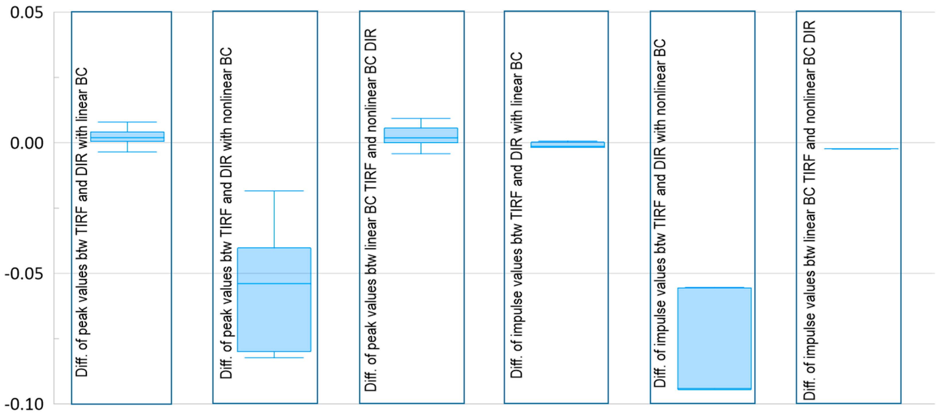
  • In Model 2 with the LNG cargo containment boxes, the dynamic shear and bending responses using the TIRF and DIR, including the linear and nonlinear boundary conditions, also matched comparatively well in terms of peak pressure and impulse values. However, the differences in the peak pressure and impulse in Model 2, using the TIRF and DIR, were found to be relatively higher than those in Model 1;
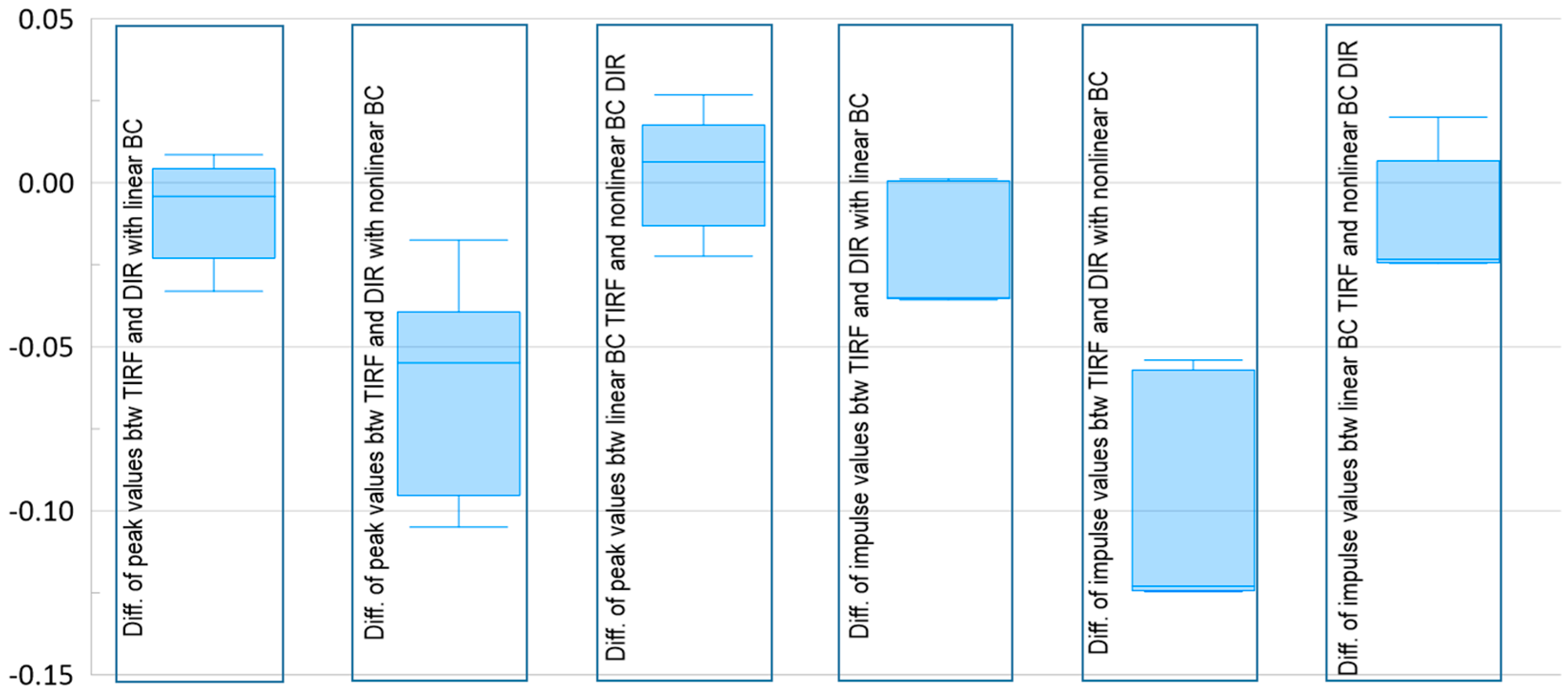
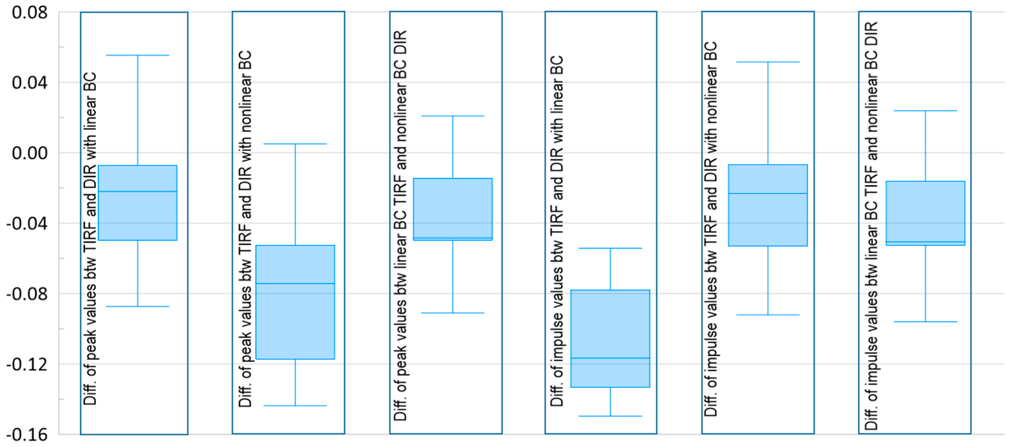
  • In Model 3, in which the hull structure was additionally included as an onboard condition, the differences in the dynamic shear and bending responses using the TIRF and DIR were found to be relatively large compared to those of Model 1 and Model 2 owing to an additional nonlinear boundary effect originating from hull deflections. However, the overall results showed good agreement with each other. The maximum difference in the peak shear response and bending response was 6.1% and 20.9%, respectively;
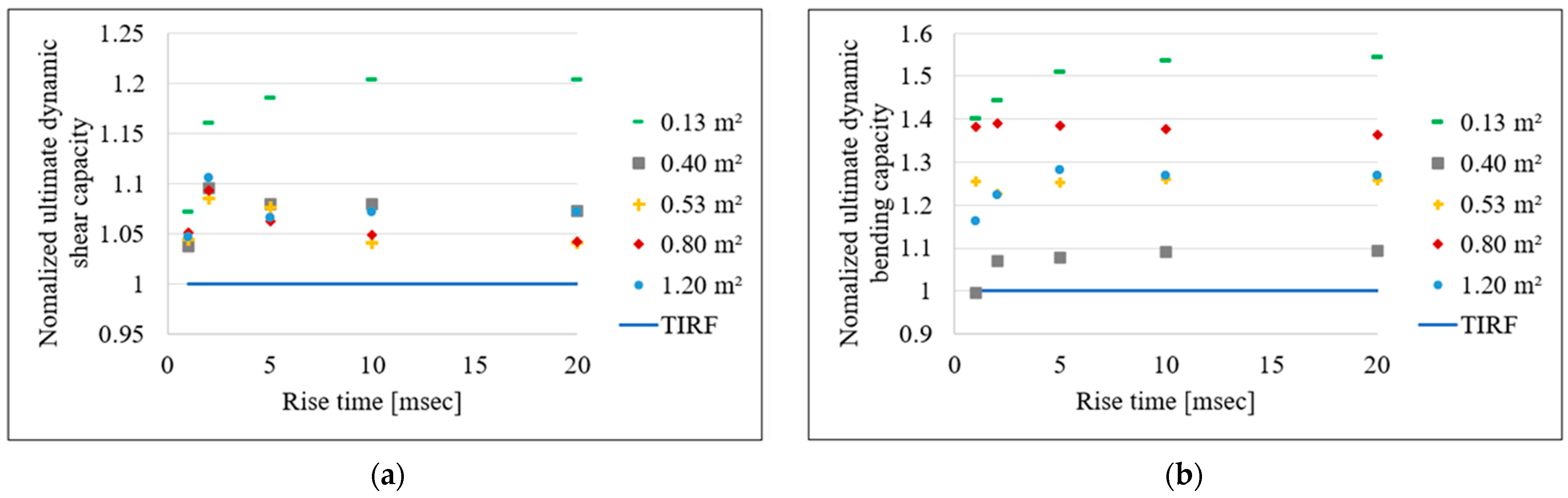
  • The design of partial material safety factors for calculating the design dynamic shear and bending capacities of an LNG cargo containment system are proposed based on the statistical analysis results from current series FE assessments;
  • Finally, the ultimate shear and bending capacities were calculated using the method proposed in this study and the results were compared with those obtained through direct nonlinear FE simulations. It showed conservative results against direct nonlinear FE simulations;
  • In this study, a simple design method based on 5h3 TIRF is presented to design the LNG cargo containment system for use in the early design stage. However, the current study was limited to the GTT NO96-type LNG cargo containment system and further study of the GTT MARK III-type system is required.

Author Contributions

Conceptualization, Y.I.P.; methodology, J.-H.K.; validation, Y.I.P.; formal analysis, S.H.L.; investigation, S.H.L.; writing—original draft preparation, J.-H.K.; writing—review and editing, Y.I.P.; visualization, S.H.L.; supervision, Y.I.P.; project administration, Y.I.P.; funding acquisition, J.-H.K. All authors have read and agreed to the published version of the manuscript.

Funding

This work was supported by the Dong-A University research fund.

Institutional Review Board Statement

Not applicable.

Informed Consent Statement

Not applicable.

Data Availability Statement

The data presented in this study are available on request from the corresponding author.

Conflicts of Interest

The authors declare no conflict of interest.

References

  1. Park, Y.I.; Kim, J. Artificial neural network based prediction of ultimate buckling strength of liquid natural gas cargo containment system under sloshing loads considering onboard boundary conditions. Ocean Eng. 2022, 249, 110981. [Google Scholar] [CrossRef]
  2. Lu, Y.; Zhou, T.; Cheng, L.; Zhao, W.; Jiang, H. Dependence of critical filling level on excitation amplitude in a rectangular sloshing tank. Ocean Eng. 2018, 156, 500–511. [Google Scholar] [CrossRef]
  3. Xue, M.A.; Zheng, J.; Lin, P.; Yuan, X. Experimental study on vertical baffles of different configurations in sup-pressing sloshing pressure. Ocean Eng. 2017, 136, 178–189. [Google Scholar] [CrossRef]
  4. Zhang, C.; Su, P.; Ning, D. Hydrodynamic study of an anti-sloshing technique using floating foams. Ocean Eng. 2019, 175, 62–70. [Google Scholar] [CrossRef]
  5. Ahn, Y.; Kim, Y.; Kim, S. Database of model-scale sloshing experiment for LNG tank and application of artificial neural network for sloshing load prediction. Mar. Struct. 2019, 66, 66–82. [Google Scholar] [CrossRef]
  6. Pilloton, C.; Bardazzi, A.; Colagrossi, A.; Marrone, S. SPH method for long-time simulations of sloshing flows in LNG tanks. Eur. J. Mech. B Fluids 2022, 93, 65–92. [Google Scholar] [CrossRef]
  7. Xue, M.A.; Jiang, Z.; Hu, Y.A.; Yuan, X. Numerical study of porous material layer effects on mitigating sloshing in a membrane LNG tank. Ocean Eng. 2020, 218, 108240. [Google Scholar] [CrossRef]
  8. Ding, S.; Wang, G.; Luo, Q. Study on sloshing simulation in the independent tank for an ice-breaking LNG carrier. Int. J. Nav. Archit. Ocean Eng. 2020, 12, 667–679. [Google Scholar] [CrossRef]
  9. Tang, Y.Y.; Liu, Y.D.; Chen, C.; Chen, Z.; He, Y.P.; Zheng, M.M. Numerical study of liquid sloshing in 3D LNG tanks with unequal baffle height allocation schemes. Ocean Eng. 2021, 234, 109181. [Google Scholar] [CrossRef]
  10. Bureau Veritas. Strength Assessment of LNG Membrane Tanks under Sloshing Loads. BV Guidance Note. 2011. Available online: https://erules.veristar.com/dy/data/bv/pdf/564-NI_2011-05.pdf (accessed on 1 September 2022).
  11. Det Norske Veritas 2009, Sloshing Analysis of LNG Membrane Tanks. DNV Classification Notes No.30.9. Available online: https://rules.dnv.com/docs/pdf/dnvpm/cn/2006-06/cn30-9.pdf (accessed on 1 September 2022).
  12. Kim, J.W.; Kim, K. Response-based evaluation of design sloshing loads for membrane-type LNG carriers. In Proceedings of the 26th International Conference on Offshore Mechanics and Arctic Engineering, San Diego, CA, USA, 10–15 June 2007; pp. 1–9. [Google Scholar]
  13. Kim, Y. Rapid response calculation of LNG cargo containment system under sloshing load using wavelet transformation. Int. J. Nav. Archit. Ocean Eng. 2013, 5, 227–245. [Google Scholar] [CrossRef] [Green Version]
  14. Nho, I.S.; Ki, M.; Kim, S. A study on Simplified Sloshing Impact Response Analysis for Membrane-Type LNG Cargo Containment System. J. Soc. Nav. Archit. Korea 2011, 48, 451–456. [Google Scholar] [CrossRef] [Green Version]
  15. Det Norske Veritas 2016, DNVGL-CG-0158, 2016, Sloshing Analysis of LNG Membrane Tanks, Class Guideline. Available online: https://global.ihs.com/doc_detail.cfm?document_name=DNVGL%2DCG%2D0158&item_s_key=00672076 (accessed on 1 September 2022).
Figure 1. Unit triangular impulse.
Applsci 13 02883 g001
Figure 2. Calculation process for the TIRF method.
Applsci 13 02883 g002
Figure 3. Schematic of the structural boundary nonlinearity in LNG CCS application. (a) Sectional view of the LNG cargo containment system; (b) Onboard condition.
Applsci 13 02883 g003
Figure 4. FE model for steel boxes with load and boundary conditions.
Applsci 13 02883 g004
Figure 5. LNG cargo containment system with 12 load cases.
Applsci 13 02883 g005
Figure 6. Boundary conditions for Model 3.
Applsci 13 02883 g006
Figure 7. Peak values (ultimate structural response) and impulse values (shaded area).
Applsci 13 02883 g007
Figure 8. Reference shear and bending responses using TIRF and DIR for impact pressure of 5.0 ms of rise time: (a) Reference shear responses with linear boundary conditions, (b) Reference bending responses with linear boundary conditions, (c) Reference shear responses with nonlinear boundary conditions, and (d) Reference bending responses with nonlinear boundary conditions.
Applsci 13 02883 g008
Figure 9. Reference shear and bending responses using TIRF and DIR for impact pressure of 10.0 ms of rise time: (a) Reference shear responses with linear boundary conditions, (b) Reference bending responses with linear boundary conditions, (c) Reference shear responses with nonlinear boundary conditions, and (d) Reference bending responses with nonlinear boundary conditions.
Applsci 13 02883 g009
Figure 10. Box and whisker plots for the difference in the peak shear stresses and impulse values using TIRF and DIR.
Applsci 13 02883 g010
Figure 11. Box and whisker plots for the difference in the peak bending stresses and impulse values using TIRF and DIR.
Applsci 13 02883 g011
Figure 12. Reference shear and bending responses for Load X (uniform pressure 3 × 3 load case) using TIRF and DIR for impact pressure of 5.0 ms of rise time: (a) Reference shear responses with linear boundary conditions, (b) Reference bending responses with linear boundary conditions, (c) Reference shear responses with nonlinear boundary conditions, and (d) Reference bending responses with nonlinear boundary conditions.
Applsci 13 02883 g012
Figure 13. Reference shear and bending responses for Load J (3 × 1 load case) using TIRF and DIR for impact pressure of 5.0 ms of rise time: (a) Reference shear responses with linear boundary conditions, (b) Reference bending responses with linear boundary conditions, (c) Reference shear responses with nonlinear boundary conditions, and (d) Reference bending responses with nonlinear boundary conditions.
Applsci 13 02883 g013
Figure 14. Reference shear and bending responses for Load A (1 × 1 load case) using TIRF and DIR for impact pressure of 5.0 ms of rise time: (a) Reference shear responses with linear boundary conditions, (b) Reference bending responses with linear boundary conditions, (c) Reference shear responses with nonlinear boundary conditions, and (d) Reference bending responses with nonlinear boundary conditions.
Applsci 13 02883 g014
Figure 15. Box and whisker plots for the difference in the peak shear stresses and impulse values using TIRF and DIR.
Applsci 13 02883 g015
Figure 16. Box and whisker plots for the difference in the peak bending stresses and impulse values using TIRF and DIR.
Applsci 13 02883 g016
Figure 17. Stress concentration through hull deflection in Model 3.
Applsci 13 02883 g017
Figure 18. Reference shear and bending responses for Load X (uniform pressure 3 × 3 load case) using TIRF and DIR for impact pressure of 5.0 ms of rise time: (a) Reference shear responses with linear boundary conditions, (b) Reference bending responses with linear boundary conditions, (c) Reference shear responses with nonlinear boundary conditions, and (d) Reference bending responses with nonlinear boundary conditions.
Applsci 13 02883 g018
Figure 19. Reference shear and bending responses for Load J (3 × 1 load case) using TIRF and DIR for impact pressure of 5.0 ms of rise time: (a) Reference shear responses with linear boundary conditions, (b) Reference bending responses with linear boundary conditions, (c) Reference shear responses with nonlinear boundary conditions, and (d) Reference bending responses with nonlinear boundary conditions.
Applsci 13 02883 g019
Figure 20. Reference shear and bending responses for Load A (1 × 1 load case) using TIRF and DIR for impact pressure of 5.0 ms of rise time: (a) Reference shear responses with linear boundary conditions, (b) Reference bending responses with linear boundary conditions, (c) Reference shear responses with nonlinear boundary conditions, and (d) Reference bending responses with nonlinear boundary conditions.
Applsci 13 02883 g020
Figure 21. Box and whisker plots for the difference in the peak shear stresses and impulse values using TIRF and DIR.
Applsci 13 02883 g021
Figure 22. Box and whisker plots for the difference in the peak bending stresses and impulse values using TIRF and DIR.
Applsci 13 02883 g022
Figure 23. Normalized ultimate dynamic capacities using TIRF and DIR: (a) Shear capacity (b) Bending capacity.
Applsci 13 02883 g023
Table 1. The design’s allowable shear and bending strengths for plywood panels [14].
9 mm12 mm
20 °C−163 °C20 °C−163 °C
M 1 c [Nmm/mm]110093518501580
M 2 c [Nmm/mm]76065013801180
Q 13 c [N/mm]59597979
Q 23 c [N/mm]43435858
Note: M 1 c = the design’s bending moment in the strong direction for the unit plate width; M 2 c = the design’s bending moment in the weak direction for the unit plate width; Q 13 c = the design’s shear stress in the strong direction for the unit plate width; and Q 23 c = the design’s shear stress in the weak direction for the unit plate width.
Table 2. Design parameters.
Model IDModelsGeometric NonlinearityBoundary NonlinearityAssessment ApproachLoad AreaRise Time
Model 1Steel boxes (1)Large deflection theoryLinearTIRFFull load (6)1 ms, 2 ms, 5 ms, 10 ms, 20 ms
DIR (5)Full load (6)
Nonlinear (4)TIRFFull load (6)
DIR (5)Full load (6)
Model 2CCS (2)LinearTIRF12 cases (7)
DIR (5)12 cases (7)
Nonlinear (4)TIRF12 cases (7)
DIR (5)12 cases (7)
Model 3CCS + Hull (3)LinearTIRF12 cases (7)
DIR (5)12 cases (7)
Nonlinear (4)TIRF12 cases (7)
DIR (5)12 cases (7)
Note: (1) two steel boxes (Figure 4), (2) LNG cargo containment boxes, (3) LNG cargo containment boxes with hull structures, (4) Nonlinear boundary condition (surface-to-surface contact condition), (5) Nonlinear dynamic transient FE assessment, (6) uniform pressure on the top of the structure, (7) 12 load cases (Figure 5).
Table 3. Material properties of the plywood panels [15].
ParameterTemperature
20 °C−163 °C
Em,1 [MPa]945013,200
Em,2 [MPa]800011,200
Em,3 [MPa]8201800
Gm,12 [MPa]7902900
Gm,13 [MPa]325700
Gm,23 [MPa]260550
ν120.10.1
ν130.10.1
ν230.10.1
Eb,1 9 mm [MPa]10,95015,350
Eb,2 9 mm [MPa]65509150
Eb,1 12 mm [MPa]10,45014,650
Eb,2 12 mm [MPa]70009800
Density [ton/mm3]6.8 × 10−106.8 × 10⁻¹⁰
Table 4. Shear responses for steel boxes (Model 1).
SHEAR RESPONSEPEAK DIFF.IMP. DIFF
Rise Time
[msec]
Peak Value (Linear)Peak Value (Nonlinear)Impulse (Linear)Impulse (Nonlinear)[2)-1)]/2)][4)-3)]/4)[4)-1)]/4)[6)-5)]/6)[8)-7)]/8)[8)-5)]/8)
TIRF (Shear) 1)DIR (Shear) 2)TIRF (Shear) 3)DIR (Shear) 4)TIRF (Shear) 5)DIR
(Shear) 6)
TIRF (Shear) 7)DIR (Shear) 8)
[N/mm][Nmm msec/mm]
14.284.324.404.324.304.304.524.290.8%−1.8%0.9%0.1%−5.5%−0.3%
24.294.304.484.318.508.508.988.500.4%−4.0%0.6%0.0%−5.6%0.1%
34.274.284.494.2812.7512.7413.9212.720.2%−4.9%0.3%−0.1%−9.4%0.2%
54.264.264.514.2621.2521.2123.1921.200.0%−5.9%0.0%−0.2%−9.4%0.2%
104.254.244.584.2442.4842.4046.3942.38−0.4%−8.0%−0.4%−0.2%−9.4%0.2%
204.234.244.594.2484.9584.8092.7784.760.2%−8.2%0.1%−0.2%−9.5%0.2%
Max0.8%−1.8%0.9%0.1%−5.5%0.1%
Note: IMP. = impulse value, DIFF = difference.
Table 5. Bending responses for steel boxes (Model 1).
SHEAR RESPONSEPEAK DIFF.IMP. DIFF
Rise Time
[msec]
Peak Value (Linear)Peak Value (Nonlinear)Impulse (Linear)Impulse (Nonlinear)[2)-1]/2)][4)-3)]/4)[4)-1]/4)[6)-5)]/6)[8)-7)]/8)[8)-5)]/8)
TIRF (Shear) 1)DIR (Shear) 2)TIRF (Shear) 3)DIR (Shear) 4)TIRF (Shear) 5)DIR
(Shear) 6)
TIRF (Shear) 7)DIR (Shear) 8)
[N/mm][Nmm msec/mm]
186.5187.2688.8587.3289.0989.1994.8089.680.9%−1.7%0.9%0.1%−5.7%0.7%
286.6587.0192.5589.03168.10168.19180.79171.520.4%−3.9%2.7%0.1%−5.4%2.0%
384.6084.8190.3986.12260.39251.59285.69254.300.2%−5.0%1.8%−3.5%−12.3%−2.4%
585.5584.6491.0285.85433.83418.89476.15424.18−1.1%−6.0%0.3%−3.6%−12.3%−2.3%
1086.1584.2293.1285.03867.54838.04952.30846.94−2.3%−9.5%−1.3%−3.5%−12.4%−2.4%
2086.4583.6893.4484.561735.011675.741904.601693.46−3.3%−10.5%−2.2%−3.5%−12.5%−2.5%
Max0.9%−1.7%2.7%0.1%−5.4%2.0%
Table 6. Shear responses for LNG cargo containment boxes (Model 2).
Rise Time [msec]Area [m2]Peak (Linear) [N/mm]Peak (Nonlinear) [N/mm]Impulse (Linear) [Nmsec/mm]Impulse (Nonlinear) [Nmsec/mm]Peak DIFF.Impulse DIFF.
TIRF 1)DIR 2)TIRF 3)DIR 4)TIRF 5)DIR 6)TIRF 7)DIR 8)[2)-1)]/2)[4)-3]/4)[4)-1]/4)[6)-5)]/6)[-8)-7)]-8)[8)-5)]-8)
10.1356.259.558.759.355.056.160.756.35.5%1.0%5.2%2.1%−7.8%2.4%
0.4055.557.357.357.155.455.058.055.03.1%−0.4%2.8%−0.8%−5.4%−0.8%
0.5356.056.757.456.555.855.059.454.91.2%−1.6%0.8%−1.4%−8.3%−1.6%
0.8056.056.657.456.456.055.059.354.91.1%−1.9%0.7%−1.8%−8.0%−2.0%
1.2051.350.952.050.753.151.655.951.6−0.7%−2.7%−1.3%−3.0%−8.4%−2.9%
20.1355.355.859.156.0109.1108.5121.3108.61.0%−5.5%1.4%−0.5%−11.7%−0.5%
0.4055.554.657.154.6111.1106.2114.2106.3−1.7%−4.5%−1.6%−4.6%−7.4%−4.5%
0.5355.454.358.454.3110.2105.0118.8104.8−2.0%−7.6%−2.1%−4.9%−13.3%−5.1%
0.8055.654.458.254.3110.8105.5118.1105.3−2.2%−7.2%−2.3%−5.0%−12.2%−5.2%
1.2052.251.253.950.9106.398.0111.398.0−2.0%−5.7%−2.5%−8.5%−13.6%−8.5%
50.1354.854.259.454.3272.2270.6303.2270.8−1.0%−9.3%−0.8%−0.6%−11.9%−0.5%
0.4055.553.056.953.0277.9264.9274.3264.4−4.7%−7.4%−4.8%−4.9%−7.5%−5.1%
0.5355.152.459.052.2274.5261.8296.9260.8−5.0%−12.9%−5.4%−4.8%−13.8%−5.3%
0.8055.652.758.752.5276.0262.8294.8262.0−5.1%−11.7%−5.4%−5.0%−12.5%−5.4%
1.2052.248.855.052.2265.7243.6278.8260.8−8.1%−5.3%−1.0%−9.1%−6.9%−1.9%
100.1354.654.259.554.2544.2541.2606.4541.4−0.8%−9.7%−0.7%−0.6%−12.0%−0.5%
0.4055.653.056.952.9555.9541.2568.2529.1−4.9%−7.4%−5.0%−4.9%−7.4%−5.1%
0.5355.052.456.952.2548.7529.7593.8521.7−4.9%−13.4%−5.4%−4.8%−13.8%−5.2%
0.8055.352.659.252.4551.8523.7568.2524.0−5.0%−8.4%−5.4%−5.0%−8.4%−5.3%
1.2053.148.856.948.61062.9525.71114.9969.8−8.7%−14.4%−9.2%−9.1%−15.0%−9.6%
200.1354.554.259.554.21088.61082.31212.81082.7−0.7%−9.8%−0.6%−0.6%−12.0%−0.5%
0.4055.653.056.853.01111.71059.41136.21058.1−4.9%−7.3%−4.9%−4.9%−7.4%−5.1%
0.5354.952.459.352.21097.31047.41043.31043.3−4.8%−13.6%−5.2%−4.8%0.0%−5.2%
0.8055.252.656.852.41103.51051.31136.21047.9−5.0%−8.4%−5.3%−5.0%−8.4%−5.3%
1.2053.148.855.648.61062.9974.41114.9969.8−8.7%−14.4%−9.2%−9.1%−15.0%−9.6%
Max5.5%1.0%5.2%2.1%0.0%2.4%
Table 7. Bending responses for LNG cargo containment boxes (Model 2).
Rise Time [msec]Area [m2]Peak (Linear) [N/mm]Peak (Nonlinear) [N/mm]Impulse (Linear) [Nmsec/mm]Impulse (Nonlinear) [Nmsec/mm]Peak DIFF.Impulse DIFF.
TIRF 1)DIR 2)TIRF 3)DIR 4)TIRF 5)DIR 6)TIRF 7)DIR 8)[2)-1)]/2)[4)-3]/4)[4)-1]/4)[6)-5)]/6)[-8)-7)]-8)[8)-5)]-8)
10.13681.5700.0687.2693.9666.2672.1703.8675.22.6%1.0%1.8%0.9%−4.2%1.3%
0.40783.0839.8762.1868.5749.1781.0670.2804.46.8%12.3%9.8%4.1%16.7%6.9%
0.53756.2819.7755.3853.6708.3742.0668.9773.67.7%11.5%11.4%4.5%13.5%8.4%
0.80760.6817.4757.6851.2724.0746.8773.6773.67.0%11.0%10.6%3.1%0.0%6.4%
1.20759.6806.4750.2759.3728.2751.8801.1749.25.8%1.2%0.0%3.1%−6.9%2.8%
20.13647.6663.9687.7667.81253.81281.01383.81287.12.5%−3.0%3.0%2.1%−7.5%2.6%
0.40740.6778.0632.1800.91421.61499.71283.31541.64.8%21.1%7.5%5.2%16.8%7.8%
0.53965.8738.0622.9768.81306.71405.51083.91454.45.7%19.0%9.5%7.0%25.5%10.2%
0.80712.0744.0636.5770.21357.21431.81122.51477.44.3%17.4%7.6%5.2%24.0%8.1%
1.20719.5749.6775.4744.81383.01437.41601.31414.14.0%−4.1%3.4%3.8%−13.2%2.2%
50.13627.2640.5687.8642.53078.73194.63442.83203.92.1%−7.1%2.4%3.6%−7.5%3.9%
0.40715.3752.6636.8774.03502.03742.13201.03846.65.0%17.7%7.6%6.4%16.8%9.0%
0.53659.7706.4543.3727.23192.33512.92492.43614.46.6%25.3%9.3%9.1%31.0%11.7%
0.80683.0719.1563.8742.63330.53578.32613.03719.75.0%24.1%8.0%6.9%29.8%10.5%
1.20695.6721.6790.370,7373407.73585.04002.53514.83.6%−11.7%1.7%4.9%−13.9%3.0%
100.13620.4639.6687.9641.56141.36391.06880.86410.63.0%−7.2%3.3%3.9%−7.3%4.2%
0.40706.9752.1638.4773.06989.27486.56399.97695.76.0%17.4%8.6%6.6%16.8%9.2%
0.53647.6705.0516.8724.16363.37019.74922.87228.18.1%28.6%10.6%9.4%31.9%12.0%
0.80673.4718.8539.5741.66643.27141.65170.77382.96.3%27.2%9.2%7.0%30.0%10.0%
1.20683.6718.2798.0705.813,595.114,302.416,009.514,048.24.8%−13.1%3.1%4.9%−14.0%3.2%
200.13617.0640.0687.9641.812,274.712,782.013,759.312,824.23.6%−7.2%3.9%4.0%−7.3%4.3%
0.40702.6752.6639.2773.413,971.014,982.712,798.915,399.16.6%17.4%9.1%6.8%16.9%9.3%
0.53641.6704.2503.5723.412,715.914,156.19814.514,435.38.9%30.4%11.3%10.2%32.0%11.9%
0.80668.6716.9527.4739.713,277.414,363.110,313.914,739.56.7%28.7%9.6%7.6%30.0%9.9%
1.20683.6718.2798.0705.813,595.114,302.416,009.514,048.24.8%−13.1%3.1%4.9%−14.0%3.2%
Max8.9%30.4%11.4%10.2%32.0%12.0%
Table 8. Dimension of the LNG carrier hull structure for Model 3.
Hull Plate Thickness [mm]Longitudinal Spacing [mm]Frame Spacing [mm]Longitudinal Stiffener—Angle Type [mm]
148102800200 × 90 × 9/14
Table 9. Shear responses for LNG cargo containment boxes with hull structure (Model 3).
Rise Time [msec]Area [m2]Peak (Linear) [N/mm]Peak (Nonlinear) [N/mm]Impulse (Linear) [Nmsec/mm]Impulse (Nonlinear) [Nmsec/mm]Peak DIFF.Impulse DIFF.
TIRF 1)DIR 2)TIRF 3)DIR 4)TIRF 5)DIR 6)TIRF 7)DIR 8)[2)-1)]/2)[4)-3]/4)[4)-1]/4)[6)-5)]/6)[-8)-7)]-8)[8)-5)]-8)
10.1356.962.159.858.756.657.761.754.98.4%−2.0%3.0%1.9%−12.4%−3.1%
0.4053.156.557.456.551.952.858.552.86.2%−1.7%6.1%1.9%−10.7%1.9%
0.5352.755.757.155.650.751.760.051.65.4%−2.8%5.2%1.9%−16.2%1.9%
0.8052.855.357.055.351.051.861.052.64.6%−3.1%4.5%1.5%−15.9%3.0%
1.2047.850.451.950.446.146.854.547.15.3%−3.0%5.2%1.5%−15.7%2.1%
20.1357.657.560.854.6115.9112.7123.4107.8−0.2%−11.2%−5.4%−2.8%−14.5%−7.5%
0.4052.552.857.852.6103.9106.9116.4106.30.6%−9.8%0.3%2.8%−9.5%2.3%
0.5351.051.658.551.599.3100.7119.9101.11.1%−13.6%1.0%1.3%−18.5%1.8%
0.8051.252.059.051.8100.0105.4121.9103.81.5%−13.8%1.2%5.1%−17.5%3.7%
1.2047.147.253.247.093.0279.2109.097.80.1%−13.1%−0.2%7.8%−11.4%4.9%
50.1358.156.361.353.7291.6268.3308.4267.4−3.1%−14.1%−8.0%−4.4%−15.3%−9.0%
0.4052.253.358.053.1569.8262.4290.6265.42.1%−9.2%1.7%3.2%−9.5%2.1%
0.5350.051.059.350.8247.1267.1299.5260.11.9%−16.7%1.6%5.9%−15.1%5.0%
0.8050.352.260.252.1248.6248.5304.8265.43.6%−15.4%3.6%6.9%−14.8%6.3%
1.2046.847.446.748.4232.2559.6272.5245.71.3%3.4%3.2%6.2%−10.9%5.1%
100.1358.256.061.553.4583.8536.4616.8533.0−4.0%−15.1%−9.0%−4.3%−15.7%−9.5%
0.4052.153.758.053.1519.7522.2581.1531.82.9%−9.2%2.0%3.1%−9.3%2.3%
0.5349.752.359.652.3493.7539.0599.0522.44.9%−14.0%5.0%5.4%−14.7%5.5%
0.8050.053.760.652.3496.9539.0609.5525.36.8%−15.7%4.5%7.8%−16.0%5.4%
1.2046.748.054.447.9932.6964.71089.9959.92.7%−13.6%2.5%3.3%−13.5%2.8%
200.1358.356.061.653.21167.61117.41233.51063.0−4.2%−15.7%−9.5%−4.5%−16.0%−9.8%
0.4052.053.758.153.31039.51068.81162.01062.43.1%−8.9%2.4%2.7%−9.4%2.2%
0.5349.552.259.852.3987.31037.61198.11039.15.2%−14.2%5.3%4.9%−15.3%5.0%
0.8049.853.260.852.7993.51056.91219.01048.36.3%−15.2%5.5%6.0%−16.3%5.2%
1.2046.748.054.447.9932.6964.71089.9959.92.7%−13.6%2.5%3.3%−13.5%2.8%
Max8.4%3.4%6.1%7.8%−9.3%6.3%
Table 10. Bending responses for LNG cargo containment boxes with hull structure (Model 3).
Rise Time [msec]Area [m2]Peak (Linear) [N/mm]Peak (Nonlinear) [N/mm]Impulse (Linear) [Nmsec/mm]Impulse (Nonlinear) [Nmsec/mm]Peak DIFF.Impulse DIFF.
TIRF 1)DIR 2)TIRF 3)DIR 4)TIRF 5)DIR 6)TIRF 7)DIR 8)[2)-1)]/ 2)[4)-3]/4)[4)-1] /4)[6)-5)]/ 6)[-8)-7)]-8)[8)-5)]-8)
10.13968.01082.0854.4869.4958.81026.1879.4852.110.5%1.7%−11.3%6.6%−3.2%−12.5%
0.40670.2670.2836.5847.3663.3828.7865.8831.220.5%1.3%20.9%20.0%−4.2%20.2%
0.53655.4655.4762.5657.8646.8671.1760.0672.27.4%−15.9%0.4%3.6%−13.1%3.8%
0.80782.3782.3709.9712.1747.2818.3747.7677.210.5%0.3%−9.9%8.7%−10.4%−10.3%
1.20659.6659.6712.2713.9653.7678.3746.9679.57.3%0.2%7.6%3.6%−9.9%3.8%
20.13971.4995.4860.3846.91941.71934.61738.91623.12.4%−1.6%−14.7%−0.4%−7.1%−19.6%
0.40669.0799.3849.5825.81345.31528.81726.81564.616.3%−2.9%19.0%12.0%−10.4%14.0%
0.53653.0656.2733.7669.41299.21290.71520.01338.80.5%−9.6%2.5%−0.7%−13.5%3.0%
0.80746.3790.9737.6674.71438.91602.71530.61325.65.6%−9.3%−10.6%10.2%−15.5%−8.5%
1.20659.6664.2729.6676.91316.11274.51493.91296.70.7%−7.8%2.6%−3.3%−15.2%−1.5%
50.13973.5966.8863.8812.34871.14790.74333.33985.0−0.7%−6.3%−19.8%−1.7%−8.7%−22.2%
0.40673.0764.0857.4783.23376.23748.64313.73899.711.9%−9.5%14.1%9.9%−10.6%13.4%
0.53651.6647.2749.5656.23252.23168.13800.03264.4−0.7%−14.2%0.7%−2.7%−16.4%0.4%
0.80725.0798.1754.2658.23560.63878.63826.53325.29.2%−14.6%−10.1%8.2%−15.1%−7.1%
1.20659.5636.1740.0647.53296.43142.03734.73319.8−3.7%−14.3%−1.9%4.9%−12.5%0.7%
100.13974.2962.0865.0797.39747.19580.18662.67913.5−1.3%−8.5%−22.2%−1.7%−9.5%−23.2%
0.40674.4754.9860.0777.26756.27584.48626.57760.210.7%−10.7%13.2%10.9%−11.2%12.9%
0.53651.1636.4754.7649.96505.56406.77600.06494.4−2.3%−16.1%−0.2%−1.5%−17.0%−0.2%
0.80717.8774.2759.8654.97110.78060.37652.96563.77.3%−16.0%−9.6%11.8%−16.6%−8.3%
1.20659.5639.2745.2653.113,189.912,732.114,938.613,007.4−3.2%−14.1%−1.0%−3.6%−14.8%−1.4%
200.13974.5962.7865.5795.219,496.619,198.417,323.215,928.4−1.2%−8.9%−22.6%−1.6%−8.8%−22.4%
0.40675.1761.1861.3781.013,514.315,128.617,252.515,501.511.3%−10.3%13.6%10.7%−11.3%12.8%
0.53650.8640.6757.4651.113,011.712,757.015,199.812,955.3−1.6%−16.3%0.0%−2.0%−17.3%−0.4%
0.80714.3797.7762.5657.814,216.116,025.415,305.813,101.910.5%−15.9%−8.6%11.3%−16.8%−8.5%
1.20659.5639.2745.2653.113,189.912,732.114,938.613,007.4−3.2%−14.1%−1.0%−3.6%−14.8%−1.4%
Max20.5%1.7%20.9%20.0%−3.2%20.2%
Table 11. Statistical data of difference in the shear/bending stresses calculated using TIRF with linear boundary conditions and DIR with nonlinear boundary conditions for Model 2 and Model 3.
Model 2Model 3
MedianMax.MeanSD.Mean ± 2 × SDMedianMax.MeanSD.Mean ± 2 × SD
Shear−2.3%5.2%−2.7%3.4%4.2,
−9.5%
2.5%6.1%1.4%4.5%10.3,
−7.5%
Bending7.6%11.4%6.6%3.5%13.6,
−0.4%
−1.0%20.9%−2.0%11.9%21.9,
−25.8%
Note: SD = Standard deviation.
Table 12. Ultimate dynamic shear capacities of Model 3 using TIRF with linear boundary condition and DIR with nonlinear boundary condition (unit: bar).
Rise Time [msec]Area = 0.13 m2Area = 0.40 m2Area = 0.53 m2Area = 0.80 m2Area = 1.20 m2
TIRFDIRTIRFDIRTIRFDIRTIRFDIRTIRFDIR
112.613.513.514.013.614.213.614.315.015.7
212.514.513.715.014.115.314.015.315.216.8
512.414.713.814.914.415.514.315.215.316.3
1012.314.813.814.914.515.114.415.115.416.5
2012.314.813.814.814.515.114.415.015.416.5
Table 13. Ultimate dynamic bending capacities of Model 3 using TIRF with linear boundary condition and DIR with nonlinear boundary condition (unit: bar).
Rise Time [msec]Area = 0.13 m2Area = 0.40 m2Area = 0.53 m2Area = 0.80 m2Area = 1.20 m2
TIRFDIRTIRFDIRTIRFDIRTIRFDIRTIRFDIR
115.221.321.921.822.428.118.826.022.325.9
215.121.821.923.422.527.619.727.422.327.3
515.122.821.923.622.528.220.328.122.328.6
1015.123.221.823.822.628.520.528.222.328.3
2015.123.321.723.722.628.420.628.122.328.3
Disclaimer/Publisher’s Note: The statements, opinions and data contained in all publications are solely those of the individual author(s) and contributor(s) and not of MDPI and/or the editor(s). MDPI and/or the editor(s) disclaim responsibility for any injury to people or property resulting from any ideas, methods, instructions or products referred to in the content.

