Influence of Headlight Level on Object Detection in Urban Traffic at Night

Abstract

The purpose of this work is to determine the influence of the low beam intensity of motor vehicle headlights on detection conditions in urban traffic. For this purpose, studies with fourteen subjects are conducted on three differently illuminated test roads, in which the low beam intensity is dimmed from off to fully on. At each dimming level, the subjects indicate whether or not they have detected the object, which is realized by a flat target and occurs at sixteen different positions in front of the vehicle. In addition, considerations of the contrast curve and the visibility level are made in order to determine the influence of switched off and fully switched on headlights. The results show that the negative contrast created by the existing street lighting creates detection conditions at least as good as full low beam intensity in almost all cases. The results further indicate that the influence of the low beam intensity increases with decreasing distance to the object and decreasing illumination levels. The results of this work show that an increase in low beam intensity initially leads to poorer detection conditions; thus, the option of reducing low beam intensity should be considered in urban traffic space.

1. Introduction

The visual system is an essential source of information for vehicle drivers in road traffic [1,2]. In order to ensure adequate visibility conditions for vehicle drivers under different lighting conditions (day and night), various lighting systems are used. On the one hand, street lighting systems are used in urban areas, which provide a lighting situation at night for all road users involved (motorists, pedestrians, cyclists). On the other hand, motor vehicle headlights are used to provide drivers with a suitable lighting situation, enabling the detection of obstacles and early reaction during driving [3].

The detection of obstacles requires a certain threshold luminance difference between the object and its environment, which depends on various factors. For example, adaptation luminance, object size, presentation time, observer age, and contrast polarity play a crucial role in object detection [1,4,5,6,7,8,9,10,11,12,13].

Several studies and analyses of traffic accident statistics show that increased adaptation luminance reduces the required contrast by increasing brightness, thereby reducing the risk of nighttime traffic accidents [14,15,16,17,18,19,20,21,22,23,24,25]. For example, analyses by Scott [26] show that in the range of roadway luminance from 0.5 to $2.0$ $\mathrm{cd}$ $\mathrm{m}$⁻² there is a direct correlation between roadway luminance and the night/day crash ratio; moreover, an increase in roadway luminance of $1.0$ $\mathrm{cd}$ $\mathrm{m}$⁻² results in a reduction in this ratio of approximately 35%. Similar results regarding the reduction of the required contrast at higher roadway or adaptation luminances can be found in studies by Damasky [13] or Blackwell [27].

Studies on the influence of object size by Aulhorn [11], Blackwell [27], and Uttley et al. [28], as well as Schmidt-Clausen [29] on the required threshold luminance difference, show that larger objects reduce the threshold luminance difference. However, it is important to distinguish between Ricco’s range, where object size has an effect, and Weber’s range, where the effect of object size is negligible [30,31].

Studies by Aulhorn [12], Blackwell and Blackwell [32], Schneider [33], and Weale [34] have demonstrated the influence of age on the detection of objects in nighttime traffic. Blackwell and Blackwell conducted a study with 235 observers of different ages. Analyzing the results for 234 of the 235 observers, they found that the visibility multiplier increases with age. Their study was performed with 4-minute Landolt rings at a background luminance of 100 $\mathrm{cd}$ $\mathrm{m}$⁻². Observers were asked to indicate recognition by a forced-choice procedure. It is noteworthy that the slope of the multiplier increased significantly from the age of 64 [32].

Contrast polarity affects the threshold luminance difference required for object detection as well [11,13,35]. Studies by Aulhorn [11] and Damasky [13] show that the threshold luminance difference for positive and negative contrast is of the same order of magnitude, and is smaller for negative contrast than for positive contrast.

These influence parameters have been incorporated into detection models by various researchers and research groups in order to make statements about the detectability of objects [30,36,37,38]. One of the most commonly used models is Adrian’s Small Target Visibility Model [30]. The threshold luminance difference $\Delta L_{th}$ is calculated according to the following formula:

$$\Delta L_{th}=k·{\left({\displaystyle \frac{\sqrt{\Phi }}{\alpha }}+\sqrt{L}\right)}^2·{\displaystyle \frac{a(\alpha ,L_B)+t}{t}}·F_{CP}·AF$$

(1)

where

• $\Delta L_{th}$: Threshold luminance difference
• k: Detection probability factor
• ${\left({\displaystyle \frac{\sqrt{\Phi }}{\alpha }}+\sqrt{L}\right)}^2$: Luminous flux and luminance function according to Ricco’s and Weber’s laws
• $\alpha$: Object size in angular minutes
• $a(\alpha ,L_B)$: Blondel-Rey constant
• t: Observation time in seconds
• $F_{CP}$: Contrast polarity factor
• $AF$: Age factor

This threshold luminance difference applies to a certain probability under laboratory conditions. To transfer this to the complexity of a real traffic situation, the Visibility Level (VL) is used as a multiplier. The VL is determined as the ratio of the currently prevailing luminance difference between the object and its background and the calculated threshold luminance difference.

In the European area, the European standard EN 13201 is used for the planning of street lighting systems, and defines the adaptation level in individual streets by specifying street lighting classes (M1 to M6), roadway luminance levels, and illuminance levels [39,40,41,42,43].

The design of motor vehicle headlights and their light distributions are regulated by international standards. It should be noted that the design of motor vehicle headlights is independent of the ambient lighting conditions. This means that when designing a low beam headlight, no distinction is made between driving on an unlit country road or highway or on an urban street illuminated by street lighting. Similarly, the design of street lighting systems does not consider the additional light provided by automotive headlights, highlighting the problem of lack of communication between automotive lighting technology and street lighting technology [39,40,41,42,43,44,45].

Especially in urban areas, the interaction of different street lighting systems and different vehicle headlight distributions creates a wide variety of lighting situations that influence detection behavior, thereby directly affecting the safety of urban road traffic at night [46,47,48,49,50].

In illuminated streets, there is a transition from negative contrast to positive contrast, as the detection object appears darker than its background due to the luminous intensity of the street lighting coming from above. This negative contrast disappears and changes into a positive contrast due to the frontal light of the vehicle headlights. The effect of this transition on detection conditions has been investigated in various studies [13,25,35,51,52,53,54,55,56,57,58,59,60,61].

Bacelar et al. [51,52] performed a study on the interaction of street lighting and automotive lighting regarding the visibility of flat detection targets. For this purpose, they positioned a flat target at a distance of 40 m in front of the vehicle on an illuminated road and determined the Visibility Level for the scenarios street lighting alone, automotive lighting alone and combination of street and automotive lighting. The results show that street lighting alone provides sufficient visibility and the addition of automotive lighting does not improve visibility. Thus, it can be concluded that street lights or low beams used alone provide better visibility than when they are used together [51]. In another study, Bacelar et al. found a correlation between the calculated Visibility Level and the subjects’ assessment of object detectability. This showed that detection objects on the roadway can be detected at a Visibility Level of 7 or higher [52].

Bullough showed that the influence of vehicle headlights depends on the illumination level of the stationary roadway lighting by determining the visibility of objects at the right edge of an illuminated roadway at 60 and 120 feet in front of the test vehicle. Thus, the influence of vehicle illumination is reduced as the illumination level on the road increases [53].

Buyukkinaci et al. conducted a study to determine the required Visibility Level for the detection of 0.2 × 0.2 m objects with different reflectance levels (0.20, 0.30, 0.40, 0.50). For this purpose, images of an illuminated street with different illumination classes (M2, M3, M4, M5) and color temperatures ( 4000 $\mathrm{K}$ and 6000 $\mathrm{K}$) were presented to 30 test subjects. The results of the study showed that a Visibility Level in the range of 7.0 to 8.5 is required in order for objects to be detected with 100% probability. Furthermore, no influence of the light spectrum on the detection was found [54].

Bhagavathula et al. studied the effect of vehicle illumination on the detectability of objects at different distances on illuminated roads. They found that there is a change in contrast polarity (positive to negative contrast and vice versa) depending on the distance in front of the vehicle. In addition, objects with negative contrast were detected at greater distances than objects with positive contrast. Furthermore, the relationship between pedestrian contrast and visibility was complex, as pedestrians showed both positive and negative contrast [35,55].

In laboratory and field studies, Damasky showed that due to the high scenario complexity in the urban area, higher contrasts are needed for the detection of objects. Furthermore, he found negative contrast results in contrast sensitivities that were up to 30% higher than those using positive contrast [13].

Studies by Akashi et al. [56] and Ekrias et al. [57] showed that the detection distance increases with increasing street lighting intensity. In addition, they concluded from their studies that the effect of the low beam on the detection conditions is high at short distances and decreases with increasing distance until no effect in nighttime urban traffic can be observed from a distance of about 80 $\mathrm{m}$ [56,57].

Vogel et al. performed photometric studies in which they calculated the Visibility Level under different light distribution ranges for different illumination classes from M3 to M6. They found that the required light distribution range depends on both the illumination class and the reflectance of the detection targets [61].

In considering subjective safety parameters, Wagner et al. found that, for a safe driving experience and detection of objects on illuminated roads, a dimmed version of the low beam can be used rather than the full intensity of the low beam, thereby reducing the energy demand of this function [58,59,60].

The studies conducted thus far show that the detection conditions in urban nighttime traffic environments depend on both street lighting and vehicle illumination. The respective effect depends mainly on the distance between the object and the vehicle. According to Bozorg et al. [62,63,64], vehicle illumination is mainly responsible for detection conditions at close range, while street lighting dominates at long range. In the intermediate range, however, both lighting systems have an influence on the prevailing detection conditions. In contrast to the majority of the considered studies, Bozorg et al. suggest designing intelligent street lighting systems and increasing their intensity. According to Bozorg et al., taking into account previously known results on the negative mutual influence of motor vehicle and street lighting [35,51,52,55,57], street lighting should be reduced in the presence of motor vehicle lighting in order to achieve the necessary detection conditions on the one hand and to strive for energy-efficient use on the other [62,63,64].

The following research questions arise from the previous research, and are answered in this paper:

(1)

What is the influence of different road illumination levels and luminous intensities of motor vehicle headlights on the detection of objects at different distances and angular positions in front of the vehicle?

(2)

What influence does the intensity of the low beam have on the contrast polarity and value of flat detection targets on illuminated roads with different illumination levels?

(3)

Is there an optimized urban light distribution for motor vehicle headlights, and if so what should it look like?

These research questions and the answers to them serve to create an understanding of the interaction between stationary street lighting and vehicle lighting. This understanding can then be used to derive requirements for future dynamically adaptive vehicle headlight distributions in order to provide drivers with the best possible detection conditions in night-time urban traffic.

Because previous studies discussed the foregoing literature review have shown that the light spectrum has no significant effect on object detection in nighttime road traffic, the present paper does not include the light spectrum as an independent study variable. As such, our investigation is limited exclusively to detection conditions varied by luminance relations.

2. Materials and Methods

The following section describes the study concept and analytical methododology of the investigation.

2.1. Test Roads

The study was conducted on three test roads located in Darmstadt, Germany, images of which are shown in Figure 1. The test roads have LED street lighting systems of different lighting classes from M4 to M6 according to EN 13201-2 [40].

The pictures of the test roads shown in Figure 1 serve as an overview of the test roads and the test setup. Photometric analysis of the test roads was performed using luminance images, which are shown schematically in Figure 2. The average roadway luminance $L_m$ varies from $0.91$ $\mathrm{cd}$ $\mathrm{m}$⁻² for test road 1 to $0.53$ $\mathrm{cd}$ $\mathrm{m}$⁻² for test road 2 and $0.38$ $\mathrm{cd}$ $\mathrm{m}$⁻² for test road 3; see Figure 2. From the luminance images, the differences in the homogeneity of the street lighting are evident, as are the different roadway brightnesses. The luminance recordings were carried out with a luminance camera (TechnoTeam LMK 5 color) attached to the rearview mirror of the test vehicle in order to realize the measurement from the driver’s point of view.

Further parameters, such as the overall uniformity $U_0$ and longitudinal uniformity $U_1$, can be found in

Table 1. Characteristics of the test roads.

Test Road	${\mathit{L}}_{\mathit{m}}$ in cd m ${}^{-2}$	${\mathit{U}}_0$	${\mathit{U}}_1$	Class
1	0.91	0.35	0.66	M4
2	0.53	0.30	0.42	M5
3	0.38	0.32	0.40	M6

.

From Table 1, it can be seen that the requirements for overall uniformity $U_0$ are not met by the three test roads. Nevertheless, these test roads were used for the investigation because the aim of this work is to consider the low beam influence on object detection at different street illumination levels.

2.2. Test Vehicle

A BMW 3 Series was used as the test vehicle for the study. The test vehicle was equipped with standard LED headlights that generate both a low beam and high beam function with LEDs. The headlights of this test vehicle were electronically modified so that they could be varied in intensity via 8-bit PWM coding. Thus, the intensity of the automotive low beam could be varied from switched off to completely switched on. Figure 3 shows the results from goniophotometer measurements of the low beam distribution at different PWM levels. Here, ${\varphi }_{\mathrm{h}}$ describes the horizontal angle of the light distribution, ${\varphi }_{\mathrm{v}}$ is the vertical angle of the light distribution, and I denotes the luminous intensity.

2.3. Test Procedure

The study was conducted with a total of 14 subjects (2 female, 12 male) who were in an age range of 25–34 years. As all test persons had to present a valid driving licence and wear a visual aid if this is noted on the driving licence, a test of visual acuity was not carried out at this point. The visual acuity test is an integral part of obtaining a driving licence in Germany, and is recognised as passed with a visual acuity of at least 0.7.

The test subjects arrived at the respective test roads and were allowed time to adapt to the currently prevailing lighting conditions during the study briefing and answering of the personality questionnaire, resulting in an adaptation time of at least 15 minutes before the actual study began. The detection objects, which were 0.2 × $0.2$ m² flat targets with a reflectance of about 4% (exact value $3.956$%), were placed on a measurement grid which had four objects per row at distances of 30 $\mathrm{m}$, 45 $\mathrm{m}$, 55 $\mathrm{m}$, and 65 $\mathrm{m}$. A low reflectance was chosen because according to studies by Randrup Hansen and Schandel Larsen [65] or Schneider [66], the clothing of pedestrians has low reflectance values of less than 10%, especially in the winter. The reflectance of the flat targets was determined by comparative measurements with a reflectance standard. Furthermore, two different vehicle positions were considered. In the first, the vehicle is placed directly under a street light system, while in the second, the vehicle is moved 10 $\mathrm{m}$ in the direction of the measurement grid, creating a second situation for the detection of objects with distances of 20 $\mathrm{m}$, 35 $\mathrm{m}$, 45 $\mathrm{m}$, and 55 $\mathrm{m}$. The applied measurement grids are shown in Figure 4.

The flat targets were horizontally separated from each other by $1.5$ $\mathrm{m}$. Those with position identifiers 3, 7, 11, and 15 were located on the longitudinal axis of the vehicle’s centerline.

The test subjects were asked to sit in the driver’s seat and focus on a fixation object consisting of a second vehicle behind the last row of objects (cf. Figure 2). The test objects were presented in randomized order, and for each test object position the intensity of the low beam function of the headlights was increased step by step. For each preset intensity of the low beam function, the test subjects signalled the detection or non-detection of the test object by a yes/no response. Subsequently, the next test object was presented and the procedure was repeated. When all sixteen test object positions had been presented at one vehicle position, the procedure continued with the second vehicle position. The start position of the test vehicle was randomized for each subject.

2.4. Measurements

For the evaluation of the study results, luminance images of all test positions in combination with the two vehicle positions were captured using a luminance camera (TechnoTeam LMK 5 color) and then analyzed. Subsequently, the Weber contrasts $C_W$ [67] (cf. Equation (3)) between object and background were calculated in order to determine the contrast curve depending on the intensity of the low beam function. For this purpose, the average value of the four bordering ambient fields was considered as the background luminance. The luminance values were then used to calculate the Visibility Levels for the test objects.

Evaluation of the subjects’ responses was carried out in three ways. First, an attempt was made to fit a psychometric function according to Linschoten et al. to the subjects’ responses [68]:

$$P\left(x\right)=\gamma +(1-\gamma )·{\displaystyle \frac{1}{1+{\left({\displaystyle \frac{x}{\alpha }}\right)}^{-\beta }}}$$

(2)

where

• $\alpha$: stimulus of the halfway point
• $\beta$: steepness of the function
• $\gamma$: probability of a positive response by chance; here, $\gamma =0$.

This evaluation methodology provides the advantage that different detection probabilities can be considered even though these probabilities may not be achieved by the headlight system used. An example of data evaluation using the psychometric function according to Linschoten et al. [68] is shown in Figure 5. Here, a psychometric function is fitted to the data with positive as well as with negative contrast; additionally the 90% threshold is plotted, and indicates secure detection.

If evaluation with the psychometric function was not possible due to the data situation, an evaluation based on the data was performed. In this case, a detection probability of 90% was assumed as a secure detection, and the setting at which this probability is permanently exceeded was considered to be the threshold. In a few cases, a data-driven evaluation was not possible either, because the detection probability of 90% was not achieved.

3. Results

This section describes the objective and subjective results of the study.

3.1. Photometric Results

First, the luminances and the corresponding Weber contrasts $C_{\mathrm{W}}$ are considered, which can be calculated according to Equation (3), where $L_{\mathrm{O}}$ represents the object luminance and $L_{\mathrm{B}}$ the background luminance [67].

$$C_{\mathrm{W}}={\displaystyle \frac{L_{\mathrm{O}}-L_{\mathrm{B}}}{L_{\mathrm{B}}}}$$

(3)

Using these data, the influence of the low beam intensity on the present contrast can be described in terms of polarity (positive or negative contrast) and value. The contrast curves obtained for the three test roads and vehicle position 1 are shown in Figure 6, Figure 7 and Figure 8. The contrast curves for vehicle position 2 are not shown here due to analogous results.

From Figure 6, Figure 7 and Figure 8, it is clear that the low beam intensity has a considerable influence on the value and polarity of the Weber contrast. At all object positions, there is initially a negative contrast between the object and its background created by the existing street lighting. If the low beam intensity is increased, a transition point from the negative contrast to the positive contrast is reached in the majority of the object positions considered on the three test roads, in which the negative contrast generated by the street lighting and the positive contrast generated by the vehicle low beam neutralize each other and no more contrast can be perceived between the object and its background. In this case, the detection object is no longer visible, and disappears for the driver. It is noticeable that the intensity of the low beam has to be increased to different extents depending on the distance and the object position in order to reach this transition point.

A further increase in the low beam intensity leads to the positive contrast gaining the upper hand on most object positions, which can make the object visible again. Again, a closer look reveals that the required increase in intensity of the low beam depends on the distance and the object position. In addition to the transition point between negative and positive contrast, the positive contrast that is exactly as large in absolute value as the initial negative contrast represents an important threshold, as between these two points the additional low beam light merely leads to a reduction in the contrast in absolute value, which worsens the visibility conditions. This condition becomes particularly critical on test road 1 with an average roadway luminance of $0.91$ $\mathrm{cd}$ $\mathrm{m}$⁻², as here this second threshold for object positions 5 to 16 cannot be reached at all with the existing headlight system. On test roads 2 ( $0.53$ $\mathrm{cd}$ $\mathrm{m}$⁻²) and 3 ( $0.38$ $\mathrm{cd}$ $\mathrm{m}$⁻²), the same applies to the objects at a distance of 65 m. In these cases, the low beam function merely causes a downgrading of the visibility conditions, and achieves the opposite of its actual function of improving visibility. This transition from negative to positive contrast is illustrated by the luminance images in Figure 9.

In the next step, the Visibility Levels are calculated for the individual object positions in the various constellations (test road and vehicle position). Based on the contrast curves from Figure 6, Figure 7 and Figure 8, this evaluation step is limited to the two boundary values, namely, low beam off and low beam fully switched on. The calculated Visibility Levels for test road 1 are shown in

Table 2. Calculated Visibility Levels for test road 1, vehicle position 1.

Low Beam off
	30 $\mathrm{m}$	45 $\mathrm{m}$	55 $\mathrm{m}$	65 $\mathrm{m}$
$-3.0$$\mathrm{m}$	33.70	24.91	17.23	13.44
$-1.5$$\mathrm{m}$	33.33	22.27	14.82	12.51
$0.0$$\mathrm{m}$	35.18	24.03	14.01	10.96
$1.5$$\mathrm{m}$	40.21	28.21	24.07	17.12
Low Beam fully switched on
	30 $\mathrm{m}$	45 $\mathrm{m}$	55 $\mathrm{m}$	65 $\mathrm{m}$
$-3.0$$\mathrm{m}$	31.87	4.00	4.03	2.92
$-1.5$$\mathrm{m}$	88.68	10.34	0.06	4.78
$0.0$$\mathrm{m}$	81.46	6.12	2.85	0.91
$1.5$$\mathrm{m}$	33.19	4.09	12.06	9.56

(vehicle position 1) and

Table 3. Calculated Visibility Levels for test road 1, vehicle position 2.

Low Beam off
	20 $\mathrm{m}$	35 $\mathrm{m}$	45 $\mathrm{m}$	55 $\mathrm{m}$
$-3.0$$\mathrm{m}$	40.16	33.11	23.38	17.99
$-1.5$$\mathrm{m}$	39.45	28.68	20.92	15.63
$0.0$$\mathrm{m}$	42.21	31.14	21.17	15.88
$1.5$$\mathrm{m}$	48.19	33.76	31.38	21.35
Low Beam fully switched on
	20 $\mathrm{m}$	35 $\mathrm{m}$	45 $\mathrm{m}$	55 $\mathrm{m}$
$-3.0$$\mathrm{m}$	31.35	16.58	6.66	5.03
$-1.5$$\mathrm{m}$	149.04	34.15	17.31	4.95
$0.0$$\mathrm{m}$	169.81	38.78	25.40	9.17
$1.5$$\mathrm{m}$	54.34	20.08	2.54	0.57

(vehicle position 2). Here, the information in the first row represents the distance in front of the vehicle and the information in the first column represents the position on the roadway, with $0.0$ $\mathrm{m}$ representing the object positions on the longitudinal axis of the vehicle’s centerline. A negative prefix means that the object was positioned to the left of this longitudinal axis and a positive prefix means that the object was positioned to the right of the longitudinal axis. It should be noted that the absolute value of the luminance difference is used to calculate the Visibility Level, which means that the Visibility Level is always positive regardless of the contrast polarity.

As shown in Table 2 and Table 3, when the low beam is off, the existing street lighting produces a higher Visibility Level at all object positions for both vehicle positions than the Visibility Level of 7 for object detection determined in previous studies [52,54]. The Visibility Level for vehicle position 1 ranges from 10.96 to 40.21, and for vehicle position 2 from 15.63 to 48.19. If the Visibility Level is now considered with the low beam fully switched on, it is noticeable that the maximum Visibility Level increases significantly. The maximum Visibility Level for vehicle position 1 is 88.68 and for vehicle position 2 it is 169.81. This means that the low beam at these positions is excessive for detecting the objects, as it is larger by a factor of about 12 to 24 compared to the Visibility Level of 7 determined in previous studies [52,54].

On the other hand, the minimum Visibility Level with fully switched on low beam is so low, with 0.06 for vehicle position 1 and 0.57 for vehicle position 2, that the luminance difference between object and background is lower than the threshold luminance difference according to Adrian’s Small Target Visibility Model [30]; thus, detection of these objects is definitely no longer possible. In addition, the Visibility Level on 9 of 16 positions for vehicle position 1 and on 5 of 16 positions for vehicle position 2 is below the Visibility Level of 7 determined in previous studies [52,54], which indicates more severe detection conditions.

Looking at

Table 4. Calculated Visibility Levels for test road 2, vehicle position 1.

Low Beam off
	30 $\mathrm{m}$	45 $\mathrm{m}$	55 $\mathrm{m}$	65 $\mathrm{m}$
$-3.0$$\mathrm{m}$	25.35	14.62	11.28	8.76
$-1.5$$\mathrm{m}$	27.75	16.47	10.31	7.23
$0.0$$\mathrm{m}$	30.14	16.42	10.75	8.21
$1.5$$\mathrm{m}$	21.80	21.03	16.73	16.00
Low Beam fully switched on
	30 $\mathrm{m}$	45 $\mathrm{m}$	55 $\mathrm{m}$	65 $\mathrm{m}$
$-3.0$$\mathrm{m}$	53.81	24.97	6.91	8.31
$-1.5$$\mathrm{m}$	74.27	23.82	8.96	6.46
$0.0$$\mathrm{m}$	116.84	31.59	14.69	10.05
$1.5$$\mathrm{m}$	93.59	23.24	12.53	2.84

and

Table 5. Calculated Visibility Levels for test road 2, vehicle position 2.

Low Beam off
	20 $\mathrm{m}$	35 $\mathrm{m}$	45 $\mathrm{m}$	55 $\mathrm{m}$
$-3.0$$\mathrm{m}$	32.83	22.16	21.38	13.34
$-1.5$$\mathrm{m}$	34.09	22.48	20.78	11.69
$0.0$$\mathrm{m}$	36.98	22.38	18.85	8.87
$1.5$$\mathrm{m}$	26.00	30.36	23.09	20.42
Low Beam fully switched on
	20 $\mathrm{m}$	35 $\mathrm{m}$	45 $\mathrm{m}$	55 $\mathrm{m}$
$-3.0$$\mathrm{m}$	70.15	52.23	18.66	9.82
$-1.5$$\mathrm{m}$	152.23	63.35	27.58	16.63
$0.0$$\mathrm{m}$	247.55	72.39	39.44	21.67
$1.5$$\mathrm{m}$	162.93	50.33	32.80	8.22

, which contain the determined Visibility Levels for test road 2, it can be seen that with the low beam switched off all object positions have Visibility Levels of more than 7 for both vehicle position 1 and vehicle position 2; thus, the visibility conditions caused by the street lighting alone should be sufficient for detecting the objects. Furthermore, it can be seen that the effectiveness of the fully switched on low beam is significantly improved for test road 2, with a lower illumination level of $0.53$ $\mathrm{cd}$/$\mathrm{m}$ compared to test road 1 ( $0.91$ $\mathrm{cd}$ $\mathrm{m}$⁻²). Thus, for both vehicle positions, there is no object position where the Visibility Level is less than 1. This means that the threshold luminance difference from Adrian’s Small Target Visibility Model is achieved with fully activated low beam for all object positions. Compared to test road 1, the number of critical object positions with Visibility Levels less than 7 decreases from 9 to 3 out of 16 positions for vehicle position 1 and from 5 to 0 for vehicle position 2.

The increase in the effectiveness of the low beam becomes even more apparent on test road 3, which is the darkest test road in the study (see

Table 6. Calculated Visibility Levels for test road 3, vehicle position 1.

Low Beam off
	30 $\mathrm{m}$	45 $\mathrm{m}$	55 $\mathrm{m}$	65 $\mathrm{m}$
$-3.0$$\mathrm{m}$	29.72	19.38	10.90	10.20
$-1.5$$\mathrm{m}$	33.23	22.59	11.55	11.00
$0.0$$\mathrm{m}$	40.42	27.04	13.55	12.10
$1.5$$\mathrm{m}$	41.50	25.45	15.75	13.80
Low Beam fully switched on
	30 $\mathrm{m}$	45 $\mathrm{m}$	55 $\mathrm{m}$	65 $\mathrm{m}$
$-3.0$$\mathrm{m}$	67.73	25.64	15.31	8.80
$-1.5$$\mathrm{m}$	135.30	27.81	18.94	9.21
$0.0$$\mathrm{m}$	94.41	28.66	15.18	6.84
$1.5$$\mathrm{m}$	74.88	26.01	17.38	10.04

and

Table 7. Calculated Visibility Levels for test road 3, vehicle position 2.

Low Beam off
	20 $\mathrm{m}$	35 $\mathrm{m}$	45 $\mathrm{m}$	55 $\mathrm{m}$
$-3.0$$\mathrm{m}$	35.55	25.72	14.26	13.59
$-1.5$$\mathrm{m}$	40.44	28.85	14.88	13.81
$0.0$$\mathrm{m}$	48.72	33.94	13.56	17.05
$1.5$$\mathrm{m}$	51.41	35.78	18.84	18.91
Low Beam fully switched on
	20 $\mathrm{m}$	35 $\mathrm{m}$	45 $\mathrm{m}$	55 $\mathrm{m}$
$-3.0$$\mathrm{m}$	56.08	33.68	15.98	8.89
$-1.5$$\mathrm{m}$	169.47	38.68	19.74	8.77
$0.0$$\mathrm{m}$	151.08	28.92	21.36	4.95
$1.5$$\mathrm{m}$	95.21	23.50	19.70	2.58

). Here, there is only one object position for vehicle position 1 and two object positions for vehicle position 2 with a Visibility Level lower than 7. On the other hand, it can be seen again that the negative contrast generated by the street lighting alone leads to a Visibility Level greater than 7 at all object positions for both vehicle position 1 and vehicle position 2, which should enable detection of the objects.

Overall, the evaluation of the visibility level on the three test roads shows the following effects. On the one hand, it becomes clear that when the low beam is switched off the Visibility Level shows less variation across the different object positions, and is greater than the proposed VL of 7 [52,54] at all considered object positions.

If the influence of the fully switched on low beam is considered, it can be seen that it strongly depends on the prevailing street lighting and the distance of the detection object to the test vehicle. The darker the road illuminated by stationary lighting systems and the shorter the distance to the detection object, the higher the Visibility Level generated by the low beam. On the other hand, the positive influence of the low beam diminishes on better illuminated roads and at greater distances. Thus, the Visibility Level generated by the street lighting alone (low beam off) establishes more robust detection conditions than the combination of street lighting and fully switched on low beam.

3.2. Subject Study Results

In the next step, the subject responses are used to consider the actual detection probabilities for the flat targets. For this purpose, the proportions of the detected flat targets in the sixteen different positions are calculated for the two cases, namely, low beam switched off and low beam fully switched on. In order to determine the proportion of detected positions, the first step is to calculate the number out of the fourteen test subjects who detect the object at each position with the low beam switched off versus with it fully switched on. This results in a certain detection probability for each object position. For example, a detection probability of $85.7$% results if 12 out of 14 test subjects detect the object. The number of object positions with a detection probability greater than the threshold considered can then be summed up. Threshold detection probabilities p of 90%, 75%, and 50% are used for this purpose. The threshold of 90% represents the threshold for secure detection, 75% the threshold for acceptable detection, and 50% the critical threshold which must not be undercut, as this means that the object is not detected in a majority of cases. The results of this consideration are shown in

Table 8. Proportion of detected objects on vehicle position 1.

Low Beam off
Test Road	p > 90%	p > 75%	p > 50%
1	15/16	16/16	16/16
2	12/16	15/16	15/16
3	14/16	16/16	16/16
Low Beam fully switched on
Test Road	p > 90%	p > 75%	p > 50%
1	6/16	7/16	12/16
2	10/16	11/16	13/16
3	12/16	14/16	15/16

for vehicle position 1 and in

Table 9. Proportion of detected objects on vehicle position 2.

Low Beam off
Test Road	p > 90%	p > 75%	p > 50%
1	16/16	16/16	16/16
2	13/16	15/16	15/16
3	14/16	16/16	16/16
Low Beam fully switched on
Test Road	p > 90%	p > 75%	p > 50%
1	12/16	13/16	16/16
2	13/16	15/16	15/16
3	15/16	16/16	16/16

for vehicle position 2.

Table 8 shows directly that with the low beam switched off in vehicle position 1, the negative contrast generated by the road lighting leads to more detected objects on all sixteen positions than the fully switched on low beam for all three test roads and all probabilities considered. This is especially evident for test road 1, with an average roadway luminance of $0.91$ $\mathrm{cd}$ $\mathrm{m}$⁻². Here, with the low beam fully switched on, only the flat targets on 6 out of 16 object positions are detected with a probability of over 90%, while with the low beam switched off the flat targets are already detected on 15 out of 16 object positions with a probability of over 90%. It is noticeable that with the low beam switched on, the detection probability for the flat targets is above the critical threshold of 50% on only 12 out of 16 positions on test road 1. Looking at the darker test roads, it can be seen that the number of objects detected with the considered probabilities are in a similar range for both switched off and fully switched on low beam.

Table 9 shows that the results for vehicle position 2 with the low beam switched off are very similar to those for vehicle position 1. On both test roads 1 and 2, one additional object position is detected with a probability of over 90%, meaning that the flat targets are now securely detected on all sixteen object positions for vehicle position 2 on test road 1, while on test road 2 this is the case for 13 out of 16 object positions. It is noticeable that in vehicle position 2 with fully switched on low beam the flat targets can be detected on more object positions than in vehicle position 1 on all three test roads. The reason for this observation can be found in the reduced distance to the object positions, as the objects are illuminated with a higher intensity when the low beam is fully switched on than when the vehicle is in position 1 due to the photometric distance law.

In addition, it is noticeable that all object positions except for one object position on test road 2 have a detection probability of at least 75% with the low beam switched off, ensuring acceptable detection. The only object position that is not detected here with a sufficient probability is object position 15, which is located directly in front of the second vehicle; this represents the fixation object, as can be seen in Figure 10. This makes the detection conditions more difficult for the test subjects, which is evident from the lower Visibility Level compared to the other object positions.

Nevertheless, it should be noted that with the low beam switched off the negative contrast generated by the street lighting alone is at least as good as the fully switched on low beam for the detection of the flat targets in almost all constellations (with the exception of vehicle position 2 on test road 3 and 90% detection probability). In many cases, the switched off low beam even leads to more detected objects out of the sixteen total object positions.

4. Discussion

This section revisits and answers the research questions raised at the outset.

(1)

What is the influence of different road illumination levels and luminous intensities of motor vehicle headlights on the detection of objects at different distances and angular positions in front of the vehicle?

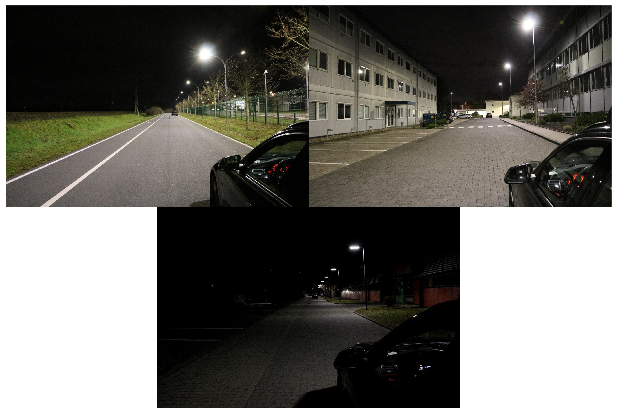
From the results of this study, it is evident that the effectiveness of the low beam is strongly dependent on the illumination level of the road, which is generated by the existing street lighting. Thus, it can be seen that on brightly illuminated roads, such as test road 1, the effectiveness of the fully switched on low beam is rather low compared to the switched off low beam, as here the existing street lighting already generates a strong negative contrast and enables the detection of the objects. This can be seen in Table 8 and Table 9; in vehicle position 1 and with low beam switched off, objects can be securely detected in 15 out of 16 positions (detection probability > 90%), while this is only possible in 6 out of 16 positions when the low beam is fully switched on. If the distance to the measuring grid is shortened (vehicle position 2), the effectiveness of the low beam increases to such an extent that objects can now be securely detected in 12 out of 16 positions. The reason for this is that at shorter distances the low beam is able to produce higher vertical illuminances on the objects, enhancing the positive contrast. Thus, the results of Akashi et al. [56], Ekrias et al. [57], and Bozorg et al. [62,63,64] can be confirmed, that is, the low beam of vehicle headlights have higher efficiency at shorter distances. In addition to the shorter distance, a lower illumination level of the road increases the effectiveness of the low beam. The proportion of securely detectable objects increases from 6 (test road 1, $0.91$ $\mathrm{cd}$ $\mathrm{m}$⁻²) to 10 (test road 2, $0.53$ $\mathrm{cd}$ $\mathrm{m}$⁻²) to 12 out of 16 positions (test road 3, $0.38$ $\mathrm{cd}$ $\mathrm{m}$⁻²) for vehicle position 1. The same trend results for vehicle position 2. Here, the number increases from 12 (test road 1) to 13 (test road 2) to 15 (test road 3) out of 16 positions with secure object detection. This correlation between the illumination level of the road and low beam effectiveness has previously been shown by Bullough [53]. Thus, the present study confirms previous findings in the literature showing that low beam effectiveness decreases as the level of illumination increases.

If the detection conditions are considered as a function of distance and object angle, no direct dependency can be determined due to the high variability and complexity of the lighting scenarios in urban traffic areas. Here, only tendencies based on the Visibility Level observation can be identified. The results for the switched off low beam on all test roads show that the object positions, which are located on the right side of the road, have higher Visibility Levels; this is because on all three test roads the street lighting systems are located on the right side. The higher Visibility Level values tend to shift to the center of the road when the low beam is fully switched on due to the light distribution of the headlights.

Thus, the findings of Bacelar [51,52], Bullough [53], Bhagavathula [35,55], Akashi et al. [56], Ekrias et al. [57], and Damasky [13] can be confirmed based on the results of the present study. While street lighting alone provides sufficient detection conditions in urban traffic areas, the combination of street lighting and automotive lighting is in many cases associated with a deterioration in detection conditions due to the resulting contrast reduction.

(2)

What influence does the intensity of the low beam have on the contrast polarity and value of flat detection targets on illuminated roads with different illumination levels?

The photometric measurements show that on all test roads there is initially a negative contrast due to the street lighting. If the intensity of the low beam is then increased, the negative contrast is initially reduced in absolute terms until a transition point is reached at which there is no longer any contrast between the object and its background. A further increase in the intensity of the low beam ensures an increase in the positive contrast. However, whether this increase reaches the same amount as the negative contrast that is present when the low beam is switched off depends to a large extent on the illumination level of the road and the distance of the object from the observer. Thus, especially when brightly illuminated roads are combined with higher distances to the detection object, there are cases in which the same amount or even the transition point from negative to positive contrast cannot be achieved; see Figure 6. Because the more brightly illuminated roads result in stronger negative contrasts, the low beam has to compensate for a significantly larger contrast range in order to produce a positive contrast. Thus, the present work confirms Bullough’s results [53], which showed that the influence of the low beam decreases with increasing illumination level. This leads to the fact that the increase in low beam intensity on many positions and test roads only leads to a reduction of the contrast amount, worsening the detection conditions.

(3)

Is there an optimized urban light distribution for motor vehicle headlights, and if so, what should it look like?

Because no direct distance or angle dependence can be determined from the data, it does not seem reasonable or possible to generate a generally valid light distribution for urban traffic areas. Moreover, the variation of street lighting is very diverse, and it is complex to consider static headlamp light distributions for optimal illumination due to differences in spacing between street lighting systems and their light point height, luminous flux, and light distribution (see AbouElhamd and Saraiji [69]). In addition, for our three test roads the negative contrast with the low beam switched off is at least as good for the detection of objects in nearly all constellations as that provided by the fully switched on low beam. Therefore, the suggestion resulting from the results of this study would be to reduce the low beam intensity, thereby enabling the detection of objects with the negative contrast. In order not to neglect the visibility of one’s own vehicle for other road users or the brightness on the roadway, forefield illumination of the vehicle would be reasonable to increase subjectively perceived safety (cf. Erkan et al. [70]). Thus, in addition to ensuring sufficient detection conditions, the driver’s sense of safety would be taken into account when generating urban headlight distributions. However, the previous authors are critical of the approach of Bozorg et al. [62,63,64] to reduce the intensity of street lighting. On the one hand, dimming the street lighting in the presence of motor vehicle lighting certainly increases the effectiveness of the low beam and improves the detectability of objects with positive contrast. On the other hand, street lighting in urban traffic areas is responsible for all road users. This includes cyclists and pedestrians as well as vehicles. A reduction in street lighting intensity could lead to a reduction in the subjective feeling of safety for these vulnerable road users, as they could receive the impression that they are no longer sufficiently visible to other road users.

5. Conclusions

In the present study, the effect of low beam intensity on contrast polarity, contrast value, Visibility Level, and object detection was investigated on three test roads (M4, M5, M6) with two vehicle and sixteen object positions. It was found that increasing the low beam intensity initially decreases the negative contrast already generated by the street lighting, and as such tends to worsen detection conditions.

These observations are confirmed by consideration of the Visibility Level. It is apparent that with the low beam switched off (maximum negative contrast) the Visibility Level for all constellations is above the value of 7 recommended in the literature [51,52,54]. When the low beam is fully switched on, the Visibility Level varies greatly between the different object positions. There are object positions with very high Visibility Levels of over 100 as well as very low Visibility Levels of 0.06. These low Visibility Levels result in a situation in which objects can no longer be detected. The study results show that the low beam effectiveness depends on various factors, such as distance to the object and the illumination level of the road. Thus, the state of research in this respect can be confirmed and extended. In the first step, the low beam initially provides worse detection conditions on illuminated roads (see Bacelar [51,52], Bhagavathula et al. [35,55]). Furthermore, the low beam effectiveness decreases with increasing distance to the object (see Bozorg et al. [62,63,64], Akashi et al. [56], Ekrias et al. [57]) and increasing road illumination levels (see Bullough [53]). Our examination of the subject data shows that in almost all constellations the switched off low beam is at least as good, and in many cases even better, for object detection than the fully switched on low beam (see Aulhorn [1,9,10,11,12,14], Damasky [13], Bhagavathula et al. [35,55]).

Therefore, it is recommended to implement the urban headlight distribution as a forefield illumination and to enable object detection primarily via the negative contrast provided by the street lighting.

Nevertheless, this work should initially be seen as a way of validating previous studies and as a further step towards fully adaptive urban light distributions for motor vehicle headlights. Because the study had to be performed on roads closed to public traffic, which were equipped with invariable street lighting, three different test roads had to be considered in order to obtain different lighting situations. This meant that the mutual influence of the vehicle lighting and the street lighting could only be examined on the basis of the variation of the low beam intensity. Other limitations of the study include the limited number and age distribution of the subjects. Moreover, it was not possible to consider the influence of the uniformity of roadway luminance due to the fixed street lighting on the three test roads. The influence of external light sources (other vehicles, moonlight, etc.) was not investigated within the scope of the present work, and would represent a useful extension of previous studies. In order to progressively consider these current limitations in follow-up studies, a fixed test road with variable street lighting would be of great interest for future investigations. The test vehicle used for the presented investigations offers the possibility of being used on any test road for further investigations. Thus, it is possible to perform further investigations on test roads with adjustable road lighting systems (light spot height, luminous flux, light distribution, light spectrum, etc.) and to specifically investigate the influence of the various parameters of light spot height, luminous flux, light distribution, and light spectrum on the detection conditions. Such a test road already exists in part, and was used for study purposes by Vogel et al. [61]. Another interesting approach is provided by Scorpio et al. [71], who are engaged in testing virtual reality (VR) environments as a possible test environment. Thus, studies could be conducted under realistic and highly controlled conditions without external disturbances. However, before VR studies can completely replace real studies, the photometric characteristics of the virtual environment need to be validated and verified.

References

1. Aulhorn, E. Ermittlung der Tauglichlichkeitsgrenzen beim Dämmerungssehen. Z. Für Verkehrssicherheit 1971, 17, 196–206. [Google Scholar]
2. Diem, C. Blickverhalten von Kraftfahrern im Dynamischen Straßenverkehr; Darmstädter Lichttechnik, Utz: München, Germany, 2005. [Google Scholar]
3. Tamburo, R.; Nurvitadhi, E.; Chugh, A.; Chen, M.; Rowe, A.; Kanade, T.; Narasimhan, S.G. Programmable Automotive Headlights. In Lecture Notes in Computer Science, Proceedings of the Computer Vision— ECCV 2014, Zurich, Switzerland, 6–12 September 2014; Fleet, D., Pajdla, T., Schiele, B., Tuytelaars, T., Eds.; Springer International Publishing: Cham, Switzerland, 2014; Volume 8692, pp. 750–765. [Google Scholar] [CrossRef] [Green Version]
4. Adrian, W. Die Unterschiedsempfindlichkeit des Auges u nd die Moglichkeit ihrer Berechnung. Lichttechnik 1968, 21, 2A–7A. [Google Scholar]
5. Adrian, W. Über den Zusammenhang zwischen Sehschwelle und Umfeldgröße. Optik 1968, 28, 132–141. [Google Scholar]
6. Adrian, W. Visibility Levels under Night-time Driving Conditions. J. Illum. Eng. Soc. 1987, 16, 3–12. [Google Scholar] [CrossRef]
7. Adrian, W. Visibility Levels in Street Lighting: An Analysis of Different Experiments. J. Illum. Eng. Soc. 1993, 22, 49–52. [Google Scholar] [CrossRef]
8. Adrian, W.; Gibbons, R. Visibility level und die Sichtbarkeit in der Straßenbeleuchtung. Licht 1993, 10, 734–739. [Google Scholar]
9. Aulhorn, E. Der Dunkelheitsunfall. In Entschließungen des 7. Deutschen Verkehrsgerichtstages in Goslar vom 30. January bis 2. February 1969; VGT: Goslar, Germany, 1969; pp. 70–78. [Google Scholar]
10. Aulhorn, E.; Harms, H. Untersuchungen über das Wesen des Grenzkontrastes. Ber. Dtsch. Ophthal. Ges. 1956, 60, 7–10. [Google Scholar]
11. Aulhorn, E. Über die Beziehung zwischen Lichtsinn und Sehschärfe. Albrecht Von Graefes Arch. Für Ophthalmol. 1964, 167, 4–74. [Google Scholar]
12. Aulhorn, E.; Harms, H. Über die Untersuchung der Nachtfahreignung von Kraftfahrern mit dem Mesoptometer. Klin. Monatsblätter Für Augenheilkd. 1970, 157, 843–873. [Google Scholar]
13. Damasky, J. Lichttechnische Entwicklung von Anforderungen an Kraftfahrzeugscheinwerfer. Ph.D. Thesis, Technische Hochschule Darmstadt, Darmstadt, Germany, 1995. [Google Scholar]
14. Aulhorn, E. Verkehrsmedizinische Risikofaktoren: Der Fußgängerunfall bei Dunkelheit. In Bericht über den 3. ADAC Ärztekongress in Hamburg vom 21. June bis 22. June 1979; ADAC Ärztekongress: Hamburg, Germany, 1979; pp. 90–99. [Google Scholar]
15. Bullough, J.D.; Donnell, E.T.; Rea, M.S. To illuminate or not to illuminate: Roadway lighting as it affects traffic safety at intersections. Accid. Anal. Prev. 2013, 53, 65–77. [Google Scholar] [CrossRef]
16. Fotios, S.; Cheal, C. Using obstacle detection to identify appropriate illuminances for lighting in residential roads. Light. Res. Technol. 2013, 45, 362–376. [Google Scholar] [CrossRef] [Green Version]
17. Fotios, S.; Gibbons, R. Road lighting research for drivers and pedestrians: The basis of luminance and illuminance recommendations. Light. Res. Technol. 2018, 50, 154–186. [Google Scholar] [CrossRef]
18. Fotios, S.; Robbins, C.J.; Uttley, J. A comparison of approaches for investigating the impact of ambient light on road traffic collisions. Light. Res. Technol. 2020, 19, 147715352092406. [Google Scholar] [CrossRef]
19. Jackett, M.; Frith, W. Quantifying the impact of road lighting on road safety—A New Zealand Study. IATSS Res. 2013, 36, 139–145. [Google Scholar] [CrossRef] [Green Version]
20. Oya, H.; Ando, K.; Kanoshima, H. A Research on Interrelation between Illuminance at Intersections and Reduction in Traffic Accidents. J. Light Vis. Environ. 2002, 26, 29–34. [Google Scholar] [CrossRef] [Green Version]
21. Sullivan, J.M.; Flannagan, M.J. The role of ambient light level in fatal crashes: Inferences from daylight saving time transitions. Accid. Anal. Prev. 2002, 34, 487–498. [Google Scholar] [CrossRef]
22. Wanvik, P.O. Effects of road lighting: An analysis based on Dutch accident statistics 1987–2006. Accid. Anal. Prev. 2009, 41, 123–128. [Google Scholar] [CrossRef]
23. Boyce, P.R.; Eklund, N.H.; Hamilton, B.J.; Bruno, L.D. Perceptions of safety at night in different lighting conditions. Light. Res. Technol. 2000, 32, 79–91. [Google Scholar] [CrossRef]
24. Boyce, P.R. The benefits of light at night. Build. Environ. 2019, 151, 356–367. [Google Scholar] [CrossRef]
25. Gibbons, R.B.; Terry, T.; Bhagavathula, R.; Meyer, J.; Lewis, A. Applicability of mesopic factors to the driving task. Light. Res. Technol. 2016, 48, 70–82. [Google Scholar] [CrossRef]
26. Scott, P.P. The Relationship Between Road Lighting Quality and Accident Frequency; TRRL Laboratory Report; Transport and Road Research Laboratory: Crowthorne, UK, 1980. [Google Scholar]
27. Blackwell, H.R. Contrast Thresholds of the Human Eye. J. Opt. Soc. Am. 1946, 36, 624. [Google Scholar] [CrossRef]
28. Uttley, J.; Fotios, S.; Cheal, C. Effect of illuminance and spectrum on peripheral obstacle detection by pedestrians. Light. Res. Technol. 2017, 49, 211–227. [Google Scholar] [CrossRef] [Green Version]
29. Schmidt-Clausen, H.J. Über das Wahrnehmen verschiedenartiger Lichtimpulse bei veränderlichen Umfeldleuchtdichten. Lichttechnik 1969, 21, 126–132. [Google Scholar]
30. Adrian, W. Visibility of targets: Model for calculation. Light. Res. Technol. 1989, 21, 181–188. [Google Scholar] [CrossRef]
31. Berek, M. Zum physiologischen Grundgesetz der Wahrnehmung von Lichtreizen. Z. Für Instrumentenkunde 1943, 63, 297–309. [Google Scholar]
32. Blackwell, O.M.; Blackwell, H.R. Individual Responses to Lighting Parameters for a Population of 235 Observers of Varying Ages. J. Illum. Eng. Soc. 1980, 9, 205–232. [Google Scholar] [CrossRef]
33. Schneider, K. Object Contrast Determination Based on Peripheral Vision Undernight-Time Driving Conditions. Ph.D. Thesis, Technische Universität, Darmstadt, Germany, 2018. [Google Scholar]
34. Weale, R. Retinal illumination and age. Trans. Illum. Eng. Soc. 1961, 26, 95–100. [Google Scholar] [CrossRef]
35. Bhagavathula, R.; Gibbons, R.; Nussbaum, M. Does the Interaction between Vehicle Headlamps and Roadway Lighting Affect Visibility? A Study of Pedestrian and Object Contrast. In Proceedings of the SAE Technical Paper Series, SAE International 400 Commonwealth Drive, Warrendale, PA, USA, April 21 2020. SAE Technical Paper Series. [Google Scholar] [CrossRef]
36. Kokoschka, S.; Gall, D. FASIVAL—Entwicklung und Validierung eines Sichtweitenmodells zur Bestimmung der Fahrersichtweite; KIT: Karlsruhe, Germany, 2000. [Google Scholar]
37. Commission International de l’Éclairage. An Analytic Model for Describing the Influence of Lighting Parameters upon Visual Performance; Publication CIE; Bureau Central de la CIE: Paris, France, 1981; Volume 19/2.1. [Google Scholar]
38. Commission International de l’Éclairage. An Analytic Model for Describing the Influence of Lighting Parameters upon Visual Performance—Volume II: Summary and Application Guidelines; Photocopy Edition; CIE: Paris, France, 1997. [Google Scholar]
39. DIN 13201-1:2005-11; Straßenbeleuchtung_- Teil_1: Auswahl der Beleuchtungsklassen. Deutsches Institut für Normung: Berlin, Germany, 2005. [CrossRef]
40. DIN EN 13201-2:2016-06; Straßenbeleuchtung_- Teil_2: Gütemerkmale; Deutsche Fassung EN_13201-2:2015. Deutsches Institut für Normung: Berlin, Germany, 2016. [CrossRef]
41. DIN EN 13201-3:2016-06; Straßenbeleuchtung_- Teil_3: Berechnung der Gütemerkmale; Deutsche Fassung EN_13201-3:2015. Deutsches Institut für Normung: Berlin, Germany, 2016. [CrossRef]
42. DIN EN 13201-4:2016-06; Straßenbeleuchtung_- Teil_4: Methoden zur Messung der Gütemerkmale von Straßenbeleuchtungsanlagen; Deutsche Fassung EN_13201-4:2015. Deutsches Institut für Normung: Berlin, Germany, 2016. [CrossRef]
43. DIN EN 13201-5:2016-06; Straßenbeleuchtung_- Teil_5: Energieeffizienzindikatoren; Deutsche Fassung EN_13201-5:2015. Deutsches Institut für Normung: Berlin, Germany, 2016. [CrossRef]
44. UNECE. ECE-R123: Uniform Provisions Concerning the Approval of Adaptive Front-Lighting Systems (AFS) for Motor Vehicles; UNECE: Geneva, Switzerland, 2013. [Google Scholar]
45. Bullough, J.D. Roadway lighting: Evolution and evaluation. In Sustainability for Road Infrastructure [Supplement to ITS International 16(6)]; Route One Publishing Ltd.: London, UK, 2011. [Google Scholar]
46. Brémond, R.; Dumont, E.; Ledoux, V.; Mayeur, A. Photometric measurements for visibility level computations. Light. Res. Technol. 2011, 43, 119–128. [Google Scholar] [CrossRef]
47. Brémond, R.; Mayeur, A. Some Drawbacks of the Visibility Level as an Index of Visual Performance while Driving. In Proceedings of the Commission Internationale de l’Eclairage (CIE)-Conference, Sun City, South Africa, 9–16 July 2011. [Google Scholar]
48. Brémond, R.; Bodard, V.; Dumont, E.; Nouailles-Mayeur, A. Target visibility level and detection distance on a driving simulator. Light. Res. Technol. 2013, 45, 76–89. [Google Scholar] [CrossRef]
49. Mayeur, A.; Bremond, R.; Bastien, J.C. The effect of the driving activity on target detection as a function of the visibility level: Implications for road lighting. Transp. Res. Part F Traffic Psychol. Behav. 2010, 13, 115–128. [Google Scholar] [CrossRef]
50. Mayeur, A.; Brémond, R.; Bastien, J.M.C. Effects of the viewing context on target detection. Implications for road lighting design. Appl. Ergon. 2010, 41, 461–468. [Google Scholar] [CrossRef]
51. Bacelar, A. The contribution of vehicle lights in urban and peripheral urban environments. Light. Res. Technol. 2004, 36, 69–76. [Google Scholar] [CrossRef]
52. Bacelar, A.; Cariou, J.; Hamard, M. Calculational visibility model for road lighting installations. Light. Res. Technol. 1999, 31, 177–180. [Google Scholar] [CrossRef]
53. Bullough, J.D.; Rea, M.S. Visibility from Vehicle Headlamps and Roadway Lighting in Urban, Suburban and Rural Locations: Sae10b; SAE International: Warrendale, PA, USA, 2010. [Google Scholar] [CrossRef]
54. Buyukkinaci, B.; Onaygil, S.; Guler, O.; Yurtseven, M.B. Determining minimum visibility levels in different road lighting scenarios. Light. Res. Technol. 2018, 50, 1045–1056. [Google Scholar] [CrossRef]
55. Bhagavathula, R.; Gibbons, R.B.; Nussbaum, M.A. Effects of Intersection Lighting Design on Nighttime Visual Performance of Drivers. LEUKOS 2018, 14, 25–43. [Google Scholar] [CrossRef]
56. Akashi, Y.; Dee, P.; Chen, J.; Derlofske, J.; Bullough, J. Interaction between fixed roadway lighting and vehicle forward lighting. In Progress in Automobile Lighting; Technical University of Darmstadt: Darmstadt, Germany, 2003; pp. 11–22. [Google Scholar]
57. Ekrias, A.; Guo, L.; Eloholma, M.; Halonen, L. Intelligent road lighting control in varying weather conditions. J. Light Eng. 2008, 16, 72–78. [Google Scholar]
58. Wagner, M.; Erkan, A.; Khanh, T.Q. Helligkeits- und Kontrastwahrnehmung bei unterschiedlichen Scheinwerfereinstellungen unter konstanter Straßenbeleuchtung. In Proceedings of the Lux Junior 2021: 15. Internationales Forum für den lichttechnischen Nachwuchs, Ilmenau, Germany, 4–6 June 2021; Tagungsband: Ilmenau, Germany, 2021; p. 297. [Google Scholar] [CrossRef]
59. Wagner, M.; Khanh, T.Q. Sicher durch die nächtliche Stadt-Helligkeits- und Kontrastwahrnehmung in der städtischen Straßenbeleuchtung aus Fahrersicht. Licht 2020, 72, 108–113. [Google Scholar]
60. Wagner, M.; Erkan, A.; Kosmas, K.; Khanh, T.Q. Reducing Head Lighting Level on Urban Roads for Different Street Lighting Situations. In Proceedings of the 13th International Symposium on Automotive Lighting (ISAL), Darmstadt, Germany, 23–25 September 2019. [Google Scholar]
61. Vogel, S.; Fiedelak, S.; Niedling, M.; Völker, S. Influence of automotive headlamp systems on the visibility of targets under different road lighting conditions. Light. Res. Technol. 2022, 64, 147715352210942. [Google Scholar] [CrossRef]
62. Bozorg Chenani, S.; Maksimainen, M.; Tetri, E.; Kosonen, I.; Luttinen, T. The effects of dimmable road lighting: A comparison of measured and perceived visibility. Transp. Res. Part F Traffic Psychol. Behav. 2016, 43, 141–156. [Google Scholar] [CrossRef]
63. Bozorg, S.; Tetri, E.; Kosonen, I.; Luttinen, T. The Effect of Dimmed Road Lighting and Car Headlights on Visibility in Varying Road Surface Conditions. LEUKOS 2018, 14, 259–273. [Google Scholar] [CrossRef] [Green Version]
64. Bozorg, S.; Bullough, J.D. Perspectives on Intelligent Road Lighting Control. J. Sci. Technol. Light. 2022, 45, 7–21. [Google Scholar] [CrossRef]
65. Randrup Hansen, E.; Schandel Larsen, J. Reflection factors for pedestrian’s clothing. Light. Res. Technol. 1979, 11, 154–157. [Google Scholar] [CrossRef]
66. Schneider, D. Markierungslicht—Eine Scheinwerferlichtverteilung zur Aufmerksamkeitssteuerung und Wahrnehmungssteigerung von Fahrzeugführern. Ph.D. Thesis, Darmstädter Lichttechnik, Technische Universität Darmstadt, Darmstadt, Germany, 2011. [Google Scholar]
67. Fechner, G.T. Elemente der Psychophysik: Erster Theil; Breitkopf und Härtel: Leipzig, Germany, 1860. [Google Scholar]
68. Linschoten, M.R.; Harvey, L.O.; Eller, P.M.; Jafek, B.W. Fast and accurate measurement of taste and smell thresholds using a maximum-likelihood adaptive staircase procedure. Percept. Psychophys. 2001, 63, 1330–1347. [Google Scholar] [CrossRef]
69. AbouElhamd, A.R.; Saraiji, R. A Contrast Based Calculation Method for Roadway Lighting. LEUKOS 2018, 14, 193–211. [Google Scholar] [CrossRef]
70. Erkan, A.; Babilon, S.; Hoffmann, D.; Singer, T.; Vitkov, T.; Khanh, T.Q. Determination of Speed-Dependent Roadway Luminance for an Adequate Feeling of Safety at Nighttime Driving. Vehicles 2021, 3, 821–839. [Google Scholar] [CrossRef]
71. Scorpio, M.; Laffi, R.; Masullo, M.; Ciampi, G.; Rosato, A.; Maffei, L.; Sibilio, S. Virtual Reality for Smart Urban Lighting Design: Review, Applications and Opportunities. Energies 2020, 13, 3809. [Google Scholar] [CrossRef]
Figure 1. Test roads on which the study was conducted: (top left) test road 1 (M4 class); (top right) test road 2 (M5 class); (bottom) test Road 3 (M6 class).
Applsci 13 02668 g001
Figure 2. Luminance images of the test roads on which the study was conducted: (top left) test road 1 ( 0.91 cd m −2, M4 class); (top right) test road 2 ( 0.53 cd m −2, M5 class); (bottom) test Road 3 ( 0.38 cd m −2, M6 class). From the luminance images, the homogeneity differences are obvious.
Applsci 13 02668 g002
Figure 3. Dimmed low beam distributions of the BMW 3 Series LED headlight used in the tests; PWM dimming changes the absolute intensity of the low beam distribution, while the light distribution itself remains unaffected by the dimming.
Applsci 13 02668 g003
Figure 4. Test setup for the detection investigations: (left) measurement grid with four flat targets each at distances of 30 m, 45 m, 55 m, and 65 m; (right) measurement grid with four flat targets each at distances of 20 m, 35 m, 45 m, and 55 m. The numbers on the flat targets indicate the internal position identifier.
Applsci 13 02668 g004
Figure 5. Example of data evaluation using the psychometric function acoording to Linschoten [68].
Applsci 13 02668 g005
Figure 6. Contrast curves on test road 1 ( 0.91 cd m −2) and vehicle position 1 depending on the intensity percentage from 0% (low beam off) to 100% (low beam fully switched on).
Applsci 13 02668 g006
Figure 7. Contrast curves on test road 2 ( 0.53 cd m −2) and vehicle position 1 depending on the intensity percentage from 0% (low beam off) to 100% (low beam fully switched on).
Applsci 13 02668 g007
Figure 8. Contrast curves on test road 3 ( 0.38 cd m −2) and vehicle position 1 depending on the intensity percentage from 0% (low beam off) to 100% (low beam fully switched on).
Applsci 13 02668 g008
Figure 9. Illustration of the transition from negative contrast to positive contrast; the two objects in the middle are clearly visible with the negative contrast (left), while an increase in the low beam intensity leads to a neutralization of the contrast and makes the objects disappear (center) and a further increase in the low beam intensity makes the objects visible again (right).
Applsci 13 02668 g009
Figure 10. Object position 15 on test road 2; detection conditions are made more difficult by the position of the flat target directly in front of the fixation object.
Applsci 13 02668 g010