Article

Comparison of Artificial Neural Network and Regression Models for Filling Temporal Gaps of Meteorological Variables Time Series

1
Institute of Monitoring of Climatic and Ecological System SB RAS, Tomsk 634055, Russia
2
Laboratory of ecosystem-atmosphere interactions in forest-bog complexes, Yugra State University, Khanty-Mansiysk 628012, Russia
3
A. M. Obukhov Institute of Atmospheric Physics, Moscow 119017, Russia
Appl. Sci. 2023, 13(4), 2646; https://doi.org/10.3390/app13042646
Submission received: 12 January 2023 / Revised: 3 February 2023 / Accepted: 15 February 2023 / Published: 18 February 2023
(This article belongs to the Special Issue Scientific Data Processing and Analysis)

Abstract

:
Continuous meteorological variable time series are highly demanded for various climate related studies. Five statistical models were tested for application of temporal gaps filling in time series of surface air pressure, air temperature, relative air humidity, incoming solar radiation, net radiation, and soil temperature. A bilayer artificial neural network, linear regression, linear regression with interactions, and the Gaussian process regression models with exponential and rational quadratic kernel were used to fill the gaps. Models were driven by continuous time series of meteorological variables from the ECMWF (European Centre for Medium-range Weather Forecasts) ERA5-Land reanalysis. Raw ECMWF ERA5-Land reanalysis data are not applicable for characterization of specific local weather conditions. The linear correlation coefficients (CC) between ERA5-Land data and in situ observations vary from 0.61 (for wind direction) to 0.99 (for atmospheric pressure). The mean difference is high and estimated at 3.2 °C for air temperature and 3.5 hPa for atmospheric pressure. The normalized root-mean-square error (NRMSE) is 5–13%, except for wind direction (NRMSE = 49%). The linear bias correction of ERA5-Land data improves matching between the local and reanalysis data for all meteorological variables. The Gaussian process regression model with an exponential kernel based or bilayered artificial neural network trained on ERA5-Land data significantly shifts raw ERA5-Land data toward the observed values. The NRMSE values reduce to 2–11% for all variables, except wind direction (NRMSE = 22%). CC for the model is above 0.87, except for wind characteristics. The suggested model calibrated against in situ observations can be applied for gap-filling of time series of meteorological variables.

1. Introduction

Continuous meteorological data records are required for the study of various natural phenomena, including climate change [1,2,3,4], extreme weather events [5,6,7], ecosystem–atmosphere exchange [8,9,10], biochemical processes in peat [11], hydrology [12], and microbiology [13]. Severe weather conditions, power supply problems, instrument malfunction, or maintenance operations result in logging stoppage of meteorological variables and the appearance of gaps in the time series [14,15]. The availability of hydrometeorological data is limited in northern latitudes because of a sparse monitoring network, harsh weather, and the high cost of experiments and instrument maintenance in these environments [16,17]. Weather stations located directly in peatland areas are unique and rare, while peatlands are characterized by a specific local climate [16,17,18,19].
A range of methods of gap-filling in the meteorological time series are used, e.g., simple arithmetic mean, regional weighting method [20], regression model [15,21,22], artificial neural network [23,24,25], machine learning [26,27,28,29,30], process parametrization model [31,32], look-up tables [33,34], downscaling of continuous dataset [35,36,37], etc. Gunawardena et al. [15] present an overview of many of these methods.
The statistical downscaling approach [37] is the building of an empirical link between the large-scale and local-scale climate, identifying and applying a statistical model to climate model output. The downscaling of meteorological variables can be applied for gap-filling of local climate data. The downscaling of global reanalysis data allowed us to obtain local or high-resolution gridded data for various meteorological variables [21,22,38,39,40]. The Coordinated Downscaling Experiment (CORDEX) [41] of the World Climate Research Programme resulted in a vast number of bias-corrected national and global climate change projections. Statistical downscaling with varying levels of complexity were developed to correct the reanalysis and global climate model simulations [37,38]. Distribution mapping or quantile mapping is a distribution-based approach that corrects the mean and variance together with wet day frequencies and intensities [22]. The combining of dynamic downscaling with convolution neural network [39] allowed us to obtain long-term high-resolution precipitation datasets in complex-terrain areas of the Tibetan Plateau.
Filling the gaps in meteorological data measured at site level using the corrected continuous data available globally was developed by [35], and it showed good performance except for the wind speed field. The gap-filling methods based on reference time series from a neighboring weather station’s products tested by [20] had good performance for gap-filling meteorological datasets with less than 40% of values missing. The use of a refence series obtained from remote sensing reduces the probability of unfilled gaps.
Gap-filling of soil moisture data for Southern Europe [42] using linear, cubic, and autoregressive interpolation and support vector machine methods showed a good ability of the model to estimate soil moisture values in the temporal, but not spatial domain. Adaptation of generalized linear models to jointly simulate several meteorological variables (air temperature, relative air humidity, global radiation, and wind speed) on a sub-daily scale was successful for surface water stress estimation in central Tunisia [43].
The various gap-filling methods are widely applied for a time series of eddy-covariance data processing [31,32,33,34,44], where gaps could typically account for 20–60% of an annual half-hourly/hourly ET dataset [45]. The look-up tables and analysis of diurnal variations of the previous periods were recommended [33] as a standard technique for gap-filling of ecosystem fluxes for EUROFLUX [8] and AmeriFlux eddy covariance databases. Later, comparison of a look-up table approach and machine learning methods applied for gap-filling of methane fluxes [34] demonstrated that decision tree algorithms performed the best in cross-validation experiments. A multiple gap-filling technique for time series of trace gases fluxes [44] and providing ensemble results of gap-filled sums will help to minimize the influence of a single technique and thus lead to a more robust flux aggregation. A full-factorial scheme proposed by [32] for gap-filling of daytime evapotranspiration can be produced hourly and daily with superior quality compared to the existing typical gap-filling methods.
Since the variations of meteorological variables are complex and nonlinear, machine learning models are powerful when implemented for problems whose resolutions require knowledge that is hard to specify [27]. Machine learning approaches could be considered as an effective and efficient technique to model meteorological processes, based on their effectiveness in modelling dynamic systems in a variety of applications of science and engineering. The data-driven models have proven to be better performance solutions in runoff modelling and flood prediction [24], terrestrial water storage [23], Arctic sea ice [46,47], incoming solar irradiance [30], precipitation [29], and other meteorological variables [14,26,27,48].
Comparison of an artificial neural network, random forest, decision tree, extreme gradient boosting, and long short-term memory algorithms [30] for the forecast of photovoltaic solar power output shows that that NNs are the most reliable and applicable algorithms resulting in the best mean absolute error, root mean squared error, and coefficient of determination. Hanoon et al. [27] indicated that in either NN architecture, there is good potential to predict daily and monthly meteorological variable values with an acceptable accuracy. Rainfall forecasting is a complicated task related to high spatial-temporal variability of precipitations. Machine learning algorithms of boosted decision tree regression and decision forest regression were successfully applied [29] for the prediction of daily, weekly, 10-day, and monthly rainfall sums at Terengganu, Malaysia. A gradient-boosting-based model applied to the Arctic sea ice area [46] produced the most unbiased, precise, and robust estimates when compared to alternative estimates, such as monthly mean albedo values or estimates from monthly linear regression models. Integration of machine learning techniques (deep-learning neural networks, generalized linear model, and gradient boosting machine) and eight climatic and hydrological input variables was successfully applied [23] to fill gaps and reconstructed the terrestrial water storage at both global grid and basin scales.
The main limitations of these more sophisticated gap-filling methods are the lack of standard tools for evaluating their performances and a non-standardized application. Implementation of a specific gap-filling method should be preceded by the investigation and comparison of the various techniques most suitable for application, taking into consideration the structure of available meteorological time series. The motivation of the present study was in the development of continuous time series for automated weather station operation since 2010 in a typical West Siberian peatland in Russia. The obtained in situ data records have large and frequent gaps. The present work is aimed to compare various regression models and an artificial neural network for the reconstruction of a temporal series of meteorological data and to choose the model for further application. The model comparison should be based on objective numerical estimations.

2. Materials and Methods

2.1. In Situ Meteorological Data

The Mukhrino field station is located in the central part of West Siberia in the middle taiga bioclimatic zone, 20 km south-west of Khanty-Mansiysk city, on the second terrace of the left bank of the Irtysh River (near the confluence with the Ob River). The Mukhrino field station research area is located in the north-east part of the Mukhrino pristine mire complex which covers a total area ~75 km2 [10]. Hydrometeorological data are available for the Mukhrino field station from 2010 to 2020 for boreal raised peatland in typical microlandscape forms. Data on air temperature, air humidity, atmospheric pressure, wind speed and direction, incoming and outgoing shortwave radiation, net radiation, and soil heat flux were recorded at automated weather stations [49].
An air temperature and humidity probe was covered by a naturally ventilated ROTRONIC AC1000 radiation shield (ROTRONIC, Bassersdorf, Switzerland). An atmospheric pressure sensor was mounted inside the enclosure case for the data logger. Wind speed and direction sensors were installed on a 10 m mast at the ridge site and a 2 m tripod at the hollow site. The distance between the mast and tripod is about 15 m. Net radiation, upward and downward photosynthetically active radiation (PAR) sensors were mounted at each site on a 2 m support crossarm, CM200, with a levelling fixture. Soil temperature at 5 cm depth was measured using an averaging soil thermocouple probe TCAV (Campbell Sci. Inc., Logan, UT, USA).
All meteorological variable time series were collected and stored in the data loggers at the weather stations. Several times a year data was manually downloaded, rearranged, and archived at the Yurga State University. The latest data archive (2010–2020) is available for download from Zenodo—https://zenodo.org/record/4323024 (accessed on 12 December 2022) [50]. The full list of meteorological variables includes 67 items. The gap filling procedure described in the present article was tested on an eight time series with significantly different temporal dynamics. The meteorological variables are shown at Table 1. The number of available hourly data records for each meteorological variable and data range are also presented. The study period 2010–2021 contains 105,191 hourly time intervals, therefore about one half of the data records are missed.
Surface pressure dynamic is characterized by slow changes of values ranging from 965 to 1062 hPa with higher readings in winter due to anticyclonic weather and lower pressure during summer. Air temperature, humidity, and incoming radiation time series have strong diurnal and annual cycles (Figure 1). Wind speed and incoming radiation can only be positive. Wind direction oscillates within the range from 0 to 360 degrees. These physically based restrictions on the data limits are potentially difficult for reproduction by statistical models. Time series of observed meteorological variables are shown in Figure 1 (curve 2).

2.2. ERA-5 Land Reanalysis Data

The number of missing observation data in the early period of automated station operation is high. Therefore, different methods for the gap-filling procedure were tested. Continuous weather data on various meteorological characteristics are required to produce a continuous gap-free data set for calculation of correct monthly or yearly averaged data [35].
The fifth-generation of atmospheric reanalysis (ERA5-Land) from the European Centre for Medium-range Weather Forecasts (ECMWF) was chosen as a source of continuous meteorological data describing the general synoptic situation but not the local meteorological features. The ERA5 dataset showed the best performance with NASA’s most recent satellite-based dataset [51]. ERA5 updates ERA-Interim using the most recent ECMWF model [52], adopting a four-dimensional variational data assimilation system (4D-VAR). It improves the correction of satellite observations and ground-based radar [53]. Hourly data for 47 meteorological parameters (Table 2) were provided by the ECMWF, downloaded from the Climate Data Store [54] for the period from 1 January 2010 to 31 December 2021.
The dataset has a spatial resolution of 0.1° × 0.1°, which approximately corresponds to 11.1 km in latitude and 5.4 km in longitude for the study area. The ERA5-Land time series for a grid point with coordinates 60.9° N 68.7° E was used as a reference of continuous meteorological data. It is clear that direct comparison of local observation data with the global reanalysis product is senseless, because the data sets have completely different origins and purposes. Nevertheless, ERA5-Land reanalysis reproduce regional weather conditions with reasonable accuracy. The differences in the time series of observed and reanalysis data are high, but the linear correlation is good [4,21,36,55].

2.2.1. Input Variables

Two input datasets were used to train the models. The first dataset includes all 47 parameters from the ERA5-Land reanalysis. Some input variables have an extremely high linear correlation coefficient (r > 0.99), for example, air temperature and dew point temperature. Multiple regression models can be successively used when model input variables are linearly independent of each other [15]. Therefore, the second dataset with only 25 variables was formed. It includes the first 25 principal components from the decomposition of the initial 47 variables into orthogonal components [56]. Time series from the second dataset are not correlated according to the definition. The first 25 principal components cumulatively describe 99.4% of the variability of the initial dataset. The first dataset was marked as “ERA data” and the second as “PCA data” (principal component analysis data).
The input variables from the ERA or PCA datasets (Table 2) were used for the modelling of the target variables (Table 1). The continuously modelled time series for each target variable was constructed individually for each model. The impact of the number of input variables on the model performance was also estimated.

2.2.2. Training and Validation Datasets

Time series of observed meteorological variables were subdivided into training and validation datasets. Model parameters were estimated on the training set and its performance was assessed with the validation set. The training set includes data from 2010 to 2019, and the validation set includes observation data from 2020 to 2021. The size of the validation set was from 13 to 28% of the full observation dataset (see Figure 1) depending on the meteorological variable.

2.3. Models

Several statistical models were tested for their ability to reproduce data from observations at a weather station. Preliminary studies include the following models: linear, interactions linear, robust linear, stepwise linear, quadratic, fine/medium/coarse tree, support vector machine regression with linear, quadratic, cubic, and Gaussian kernel, the Gaussian process regression model with rational quadratic, squared exponential, Matern 5/2 and exponential kernel, and single/double/triple layered neural networks with various layer sizes. Regression models were optimized using the Regression Learner App from MATLAB software version 2022a [57]. The Regression Learner performs supervised machine learning by supplying a known set of observations of input data (predictors) and known responses. Only five models with the minimal root-mean-square error were selected for further studies: linear model (LM), linear model with interactions (LMI), Gaussian process regression model with exponential kernel (GPRexp), Gaussian process regression model with rational quadratic kernel (GPR2), and bilayer neural network (NN) were used for detailed studies. A 5-fold cross-validation was applied at model training to protect against overfitting.

2.3.1. Direct ERA5-Land Comparison

In the first step, the observed variables were directly compared to the corresponding variables from the ERA5-Land data. The ERA5- Land data are constructed from a very complex coupled atmosphere–ocean–land global model that assimilates some ground and satellite observation data. Direct comparison (ERA dataset) with in situ ground observations shows good agreement for some variables on the global scale [54]. However, at the local scale non-zero bias between ERA data and local observations exists [21].

2.3.2. De-Biased ERA5-Land Data

The ERA5-Land data have fine spatial resolution, but still require the downscaling procedure for taking into account local climate features [37]. We use simple linear scaling of the ERA data to obtain the de-biased time series:
y = a · E R A + b ,
where a and b are parameters estimated using the training dataset for each observed variable, and y is the modelled (de-biased) variable.

2.3.3. Linear Regression Models

Two types of linear regression model were tested. A simple linear model (LM):
y = i = 1 n a i · z i ,
and a linear model with interactions (LMI)
y = i = 1 n ( a i · z i + j = 1 i b i j · z i · z j ) ,
where z i are input variables from the ERA or PCA datasets, n is the number of input variables, and a i , and   b i j are model parameters estimated using the training dataset for each modelled variable y.

2.3.4. Gaussian Process Regression Models

Gaussian process regression model [58,59] with nonparametric kernel-based probabilistic models using exponential kernel (GPRexp) and rational quadratic kernel (GPR2) were selected for application basing on the results of preliminary studies.

2.3.5. Artificial Neural Network

The bilayer artificial neural network (NN) was applied for gap-filling of the time series. NN models have been utilized by many previous studies of meteorological variable gap-filling [13,24,60]. The structure of NN is composed of an input layer, two hidden layers, and an output layer. Each hidden layer has ten nodes (neurons). Additional experiments were performed with a variation of the number of hidden layers and number of neurons. The NN was trained through Bayesian regularization backward propagation. Another validation subset was selected from the initial training dataset to prevent the model overfitting. The validation subset size consisted of 15% from the training dataset.

2.4. Model Performance Estimation

Each model was trained for each target (observed) variable using the training dataset with ERA and PCA input variables. Then a time series of each target variable was constructed using the full set of input data. The performance of the models was evaluated against independent validation dataset using the normalized root-mean-square error (NRMSE), linear Pearson’s correlation coefficient (CC), and Kling–Gupta efficiency (KGE) [23,61].
The NRMSE (4) is the root-mean-square error normalized by observation data range [28]:
R M S E = 100   % x m a x x m i n i = 1 n ( y i x i ) 2 n .
The CC Equation (5) measures the strength of linear associations between modelled and observed data with value ranges between −1 and +1.
C C = i = 1 n ( ( x i x ¯ ) ( y i y ¯ ) ) i = 1 n ( x i x ¯ ) 2 i = 1 n ( y i y ¯ ) 2 .
The KGE Equation (6) is an objective performance metric combining correlation, bias, and variability [23,61].
K G E = 1 ( C C 1 ) 2 + ( y ¯ x ¯ 1 ) 2 + ( σ y σ x x ¯ y ¯ 1 ) 2 ,
where x and y represent actual and modelled time series data, x ¯ and y ¯ represent average x and y; and σ x , σ y are the standard deviation of the time series. The CC and KGE values all have their optimum at unity.

2.5. Data Processing Overview

The full flowchart of the gap-filling procedure is shown in Figure 2. The continuous input data (z) form the training subset of ERA or PCI datasets used for generating the continuous time series of modelled data (y). The modelled data are compared against the target data (x) and optimal model parameters are seeking to minimize the RMSE between the target and modelled data. The model parameter optimization in the training phase is performed by the Regression Learner App from MATLAB software. During the validation phase the model is run using the optimal model parameters determined in the training phase and the input data from the validation data set is used for the generation of the continuous modelled data. The model performance metrics (CC, NRMSE, and KGE) are calculated for the validation dataset of the modelled and target data. The model performance metrics are compared for various regression and NN models to reveal the best model for gap filling. The model training and validation procedures were repeated for five models and eight target datasets. The application phase includes the running of the best model using the full input dataset and optimal model parameters determined during the training phase. The modelled data are used for filling gaps in the training data where the observations are missed.

3. Results

3.1. Direct ERA5 Comparison

The ERA5-Land reanalysis provides meteorological variables with a 1 h time step. The linear Pearson’s correlation coefficients between the ERA5 variables and in situ observed variables are shown in Supplementary Table S1. The highest correlation coefficient values vary from 0.61 for wind direction to 0.99 for air pressure. The ERA5 variables that were used for direct comparison with local observation results are the surface pressure, temperature at 2 m, relative air humidity, and soil temperature at level 1. Wind speed and wind direction were calculated from U and V components of the wind speed at 10 m. Incoming photosynthetically active radiation was estimated from the surface solar radiation downwards divided by the constant derived from observations. The net radiation at the surface was accounted for as the sum of the surface net solar radiation and surface net thermal radiation. The results of direct comparison of variables are shown in Figure 3.
Some of the studied variables from ERA5-Land data have good agreement with in situ observations. Atmospheric pressure according to ERA5-Land data is lower than observed by 3.5 hPa, and CC is 0.99 both for training and validation datasets. The difference for air temperature is more pronounced. Long-term average air temperature according to observations is −0.5 °C and according to ERA5-Land data the temperature is −3.7 °C. The ERA5-Land data underestimated the temperature in summer as extremely high. Incoming radiation, net radiation, relative air humidity, and soil temperature are reproduced by ERA5-Land with an average quality. A ratio of observed and ERA5-Land data varies in the range from 0.75 to 1.17, and CC varies in the range from 0.83 to 0.98. The worst agreement was obtained for wind speed and wind direction. It is clear that local wind is formed by local orography conditions and it is weakly reproduced by the global circulation model. CC was 0.77 for wind speed and −0.56 for wind direction. The ERA5-Land data were denoted as model ERA and compared with observations in the following sections.
Therefore, direct use of ERA5-Land data for the describing of local weather conditions is not applicable, except for air pressure data. All other studied meteorological variables were reproduced in ERA5-Land data with serious biases. Vuichard and Papale [35] suggest a simple correction of reanalysis data. The de-biased ERA5-Land reanalysis data are denoted as the dbERA model and analyzed as with all other models in the following sections.

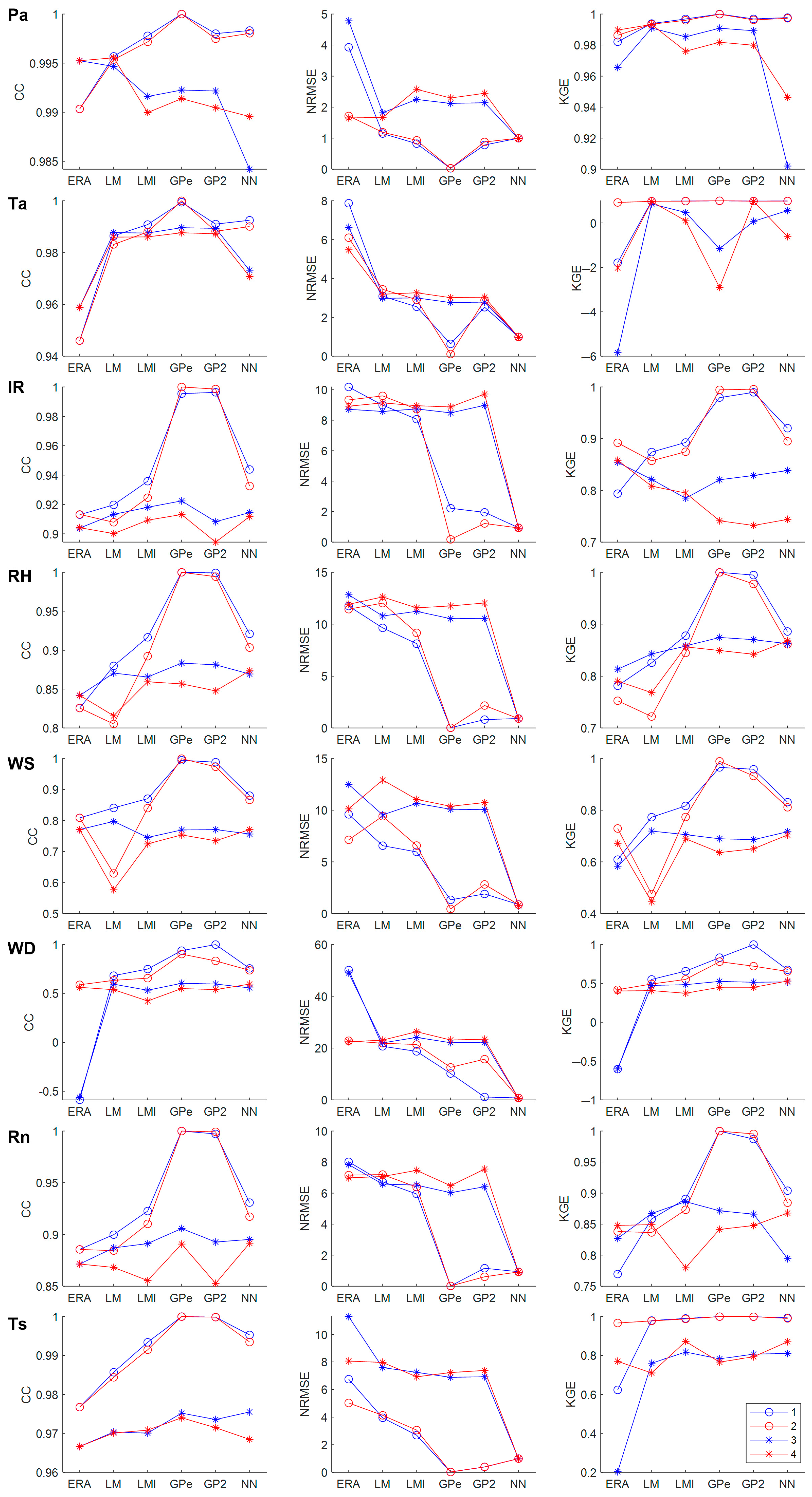
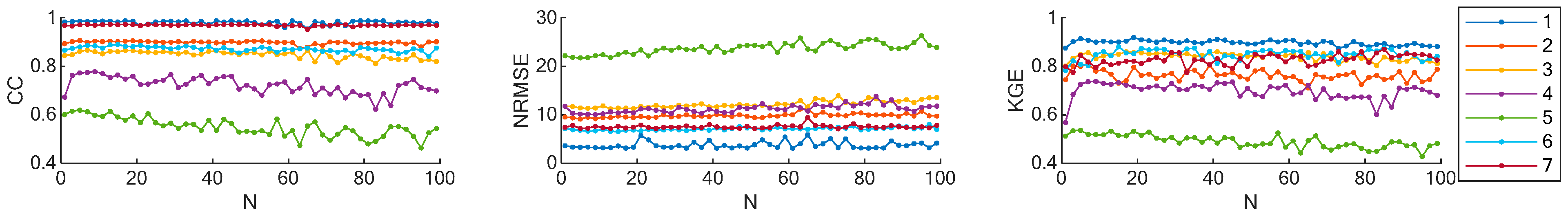
3.2. Model Performances

Figure 4 presents the results of the comparison of air temperature from in situ observations and various models. Two sets of input variables were used to train the models: the ERA dataset with 47 items and the PCA dataset with 25 items. At first glance, there are no essential differences between the models. Direct ERA data have a systematic error of about 3.2 °C. The de-biased ERA data mean value is equal to the mean observed value, but the variation of differences is still high. The regression models have smaller variation of differences. The NN models have significant negative outbursts at below zero air temperatures. The comparison of average and standard deviation for meteorological variables estimated from in situ and modelled data is shown in Supplementary Tables S2 and S3.
Figure 5 shows the performance metrics (CC, NRMSE, and KGE) for five models (LM, LMI, GPRexp, GPR2, and NN) during the testing phase (curves 1,2) and the validation phase (curves 3,4) for ERA (curves 1,3) and for PCA (curves 2,4) datasets. The dbERA model presented as points ERA at curves 3,4. The performance metrics for the testing phase are usually better than for the validation phase, due to selected calibration technique.
The atmospheric pressure is reproduced by any regression models with a relatively high accuracy. The CC values are above 0.99 for all models, except the NN model with the ERA dataset. NRMSE is about 1–2% for the validation phase, except for the direct ERA5-Land data. According to the NRMSE metric, the NN model is better than other models, but the complex KGE metric demonstrates weakness of the NN model both for the ERA and for PCA datasets.
The performance of air temperature models depends on selected performance metrics. The CC and NRMSE results in high ranks for regression models (CC > 0.98, NRMSE < 3%), and low ranks for the ERA (CC = 0.96, NRMSE = 6.6%), dbERA (CC = 0.96, NRMSE = 5.5%), and NN (CC = 0.97, NRMSE = 1%) models. The KGE metric comparison results in better performance for the LM (KGE = 0.96) and GPR2 (KGE = 0.97) models with the PCA dataset and low performance of the NN model (KGE = 0.5 and −0.6).
The incoming radiation according to modelled data has a good correlation (CC = 0.89 ± 0.92) with observation data due to diurnal patterns of radiation. NRMSE for most models is about 8.9–9.7% except the NN model that has an NRMSE of 0.9%. The KGE metric is above 0.8, but the GPR and NN models based on the PCI dataset shows lower KGE than the same models based on the ERA dataset.
CC for relative air humidity varies from 0.82 to 0.89 depending on the selected model. NRMSE is 10.6–12.6, except for the NN model with a ten time’s smaller error, as it was for the incoming radiation NN model. The difference between KGE for various models for the relative air humidity is insignificant and changes within the range of 0.77–0.87.
The linear model with PCA dataset demonstrated bad performance for simulation of the wind speed with CC = 0.58 and KGE = 0.45. All other models were good enough for modelling of the wind speed.
Estimation of model performances showed that the wind direction has the biggest errors and lowest correlation among all studied meteorological variables. The correlation coefficients are below 0.6 and have a negative value for direct ERA5-Land comparison. NRMSE is about 23–26%, except for the NN model (NRMSE = 0.6%). KGE is at an average level of 0.37–0.53.
The CC value for net radiation is high (0.86–0.9) and some improvements were obtained using the PCA dataset. The NN model demonstrated the lowest NRMSE compared with other models, and the KGE for the NN model is higher than for other models.
Similar results were obtained for modelling of the soil temperature. The NN model showed a slightly better performance than regression models and much better results than direct ERA data. The CC values for all models is high (0.97–0.98), NRMSE is about 8%, and KGE is above 0.7.

3.3. Computational Complexity

Model training, testing, and application were performed on a desktop personal computer: Intel Core i7-8700 CPU 6 × 3.2 GHz with 16 Gb RAM. The model training phase requires the most computing time compared to the testing and validation phases. The LM and LMI models were trained in 1–2 min, the NN model with 1000 epochs was trained in 2–3 min. The GPRexp/GPR2 models required about 120–240 min for the training model for a single target variable. After the optimal model parameters were identified, the computation of the continuous time series for a target variable at testing or application phase occur for 10–20 s. A 5-fold cross-validation was applied during model training to protect against overfitting. An increase in the number of iterations for cross-validation results in a rise in the computing time.

4. Discussion

4.1. Input Variables

The gap-filling models discussed in this paper showed a good approximation of the original data. The quality of modelled data depends on the applied model and the input dataset used. The ERA dataset contains 47 meteorological variables with potentially excessive information. The taking into account of some variables is useless for improvement of the model performance. Illustration of the input variables’ importance for the linear model is shown in Figure 6. The figure demonstrates changes of the model’s performance depending on the number of input variables used. The order of variables is listed in Table 2. Analysis shows that air temperature is reproduced by the linear model with good accuracy using one variable (see curve 1 in Figure 6) due to the fact that the first input variable from the ERA dataset is the temperature at 2 m. The second input variable (skin temperature) slightly increases the model’s performance according to the CC and NRMSE metrics. KGE for the air temperature with the linear model varies slightly with the application of up to 30 input variables. Implementation of more variables results in a decrease in KGE and reduces the model’s quality. Similar changes occur with an increase in the number of input variables for other meteorological parameters. The linear model for atmospheric pressure (curve 2 in Figure 3) was improved after the addition of the 33rd variable (surface pressure). The performance of the linear model for the wind speed (curve 5 in Figure 3) rises gradually with an increase in the number of inputs and then becomes higher with an addition of the 45th variable (wind speed at 10 m) from the ERA dataset. Reordering of the input variable list may significantly reduce the required number of inputs for good model training.
Similar results were obtained for other studied models. The CC and KGE for LMI, GPRexp, GPR2, or NN model increase with the rise of the number of input variables from the ERA dataset. The most significant rise of the model performance occurs after taking into account the input variable having the largest correlation coefficient with the target variable (see Table S1 in the Supplementary Materials). A further increase in the number of input variables results in a slight improvement of the model.
The principal component analysis technique was applied to reduce the dimensionality of the input data and prevent preconceived notions for input variables selection. Twenty-five new variables describing the highest variability of the initial dataset were formed into the PCA dataset. The linear correlation between target variables and PCA variables is lower than for raw ERA variables. The correlation coefficients do not exceed 0.61. An increase in the number of input variables from the PCA dataset influences the overall model performance. Figure 7 shows the model performance change with the rise in the number of inputs from the PCA dataset. The 1st PCA variable is relatively good for modelling of the air temperature (curve 1 in Figure 7). The first two input variables essentially increase the model’s performance for incoming radiation and air humidity. The model for wind speed and atmospheric pressure requires at least 10–15 PCA input variables to obtain good results and reach the performance typical for other meteorological variables.
Various models (LMI, GPRexp, GPR2, and NN) demonstrate similar results with comparison of the importance on the number of input variables. The air and soil temperature always show a better performance. The wind direction and wind speed are the most difficult variables for reproduction by any model. According to Figure 6 the increase in PCA input variable numbers above 16 variables does not result in any changes of the model’s quality.
Irvin et al. [34] demonstrated the importance of the input variable dataset for the gap-filling of the eddy-covariance derived methane fluxes for 17 FLUXNET [8] wetland sites. The marginal distribution sampling model had a good median performance even with a limited set of input variables, and artificial neural networks showed comparable performance when using all predictors.
The configuration of the NN model is more complicated than other regression models. The number of hidden layers and number of neurons (nodes) can potentially change the model performance. The optimum architecture (number and size of a hidden layer) is related to the complexity of the input and output mapping, along with the amount of noise and the size of the training data [48]. The influence of the number of hidden layers and the size of the hidden layers on the NN model’s performance were tested in the numerical experiments. The single layer, bilayered, and trilayered NN models demonstrate very close results in reproduction of meteorological variables. The number of neurons in the hidden layers does play a small role in the construction of the good NN model. Figure 8 shows the change in performance of the bilayered NN model with an increase in the size of the hidden layers from 1 to 100 neurons. It was found that a rise in the KGE indicator occurs at an increase in the number of neurons from 1 to 5. A further increase in the hidden layer size does not lead to the model’s improvement.

4.2. The Model Comparison

Five tested models were compared regarding their ability to reproduce the time series of meteorological variables using ERA and PCA datasets as input variables. First, the performance metrics (CC, NRMSE, and KGE) were averaged for eight target variables. Table 3 shows the average CC, NRMSE, and KGE values for each model. Second, a rank estimation was assigned for each model and each performance metric. For instance, the GPRexp model based on the ERA dataset with the highest CC = 0.91 ranked 100 for the CC metric, and the GPR2 model based on the PCA dataset with CC = 0.89 ranked 0. All other models ranked between 0 and 100 according to the CC values. Similar ranks were assigned for the NRMSE and KGE metrics. Finally, mean rank (MER) for the CC, NRMSE, and KGE parameters was used as a final and complex model estimation (Table 3). According to the suggested approach, the GPRexp model with ERA input variables demonstrated the best results for all the studied meteorological time series. It should be noted, that all performance estimations were made on an independent validation dataset not used for the model training.
The model performance for the training dataset was also estimated and is shown in Figure 5 (curves 1,2). It is clear, that the training subset demonstrates a better quality of target variables modelling than the validation subset. CC for GPRexp and GPR2 models are extremely high (above 0.995) for all target variables. The LM and LMI models demonstrate a higher CC and KGE for the training subset than for the validation ones. While, the NRMSE for linear models does not change significantly between the training and validation subsets, the exceptions are atmospheric pressure and soil temperature variables. The NRMSE value for the training dataset of the GPRexp and GPR2 models is less than 1%. A very small NRMSE was also obtained for the NN model both for the training and validation subsets. Choice of ERA or PCA datasets does not impact on the NN model’s performance.
All models indicated a slightly lower performance during the testing phase than in the training phase. The performance for the linear model slightly improves after transition from training phase to testing phase. The performance for the Gaussian process regression model changed significantly. The NN models do not change NRMSE and KGE metrics, while CC for the validation dataset is lower than for training for all studied meteorological variables.
In general, all the models studied in this work have proven to be valid gap-filling techniques for the meteorological time series. However, some of them reconstructed the time series with greater precision. The worst coincidence was obtained between raw ERA5-Land data and the observed in situ data. The linear bias correction of the ERA5-Land data (dbERA model) improves the data reproduction quality in terms of MER from 12 to 54 (Table 3). The performance of the linear bias correction method across global sites [35] applied for ERA-Interim data reduces the mismatch with the in situ data by 10 to 36%, depending on the meteorological variable considered. The authors [35] report on the poor performance of the bias correction method for wind speed. The dbERA model tested at the present study was rather good for the wind speed variable and even for wind direction. The largest increment for the KGE value was obtained after bias correction of the wind speed and soil temperature variables. It claims that these variables at local scale do not have strong connections with the raw ERA5-Land data.
The linear models with the ERA input dataset work better than the raw or debiased ERA5-Land data. The median model ranks are 83 and 80 for the LM and LMI models, respectively. The LM model showed the best results of all models in the KGE metric. An increase in the linear model complexity after implementation of interactions (LMI model) does not increase the model’s performance. Two tested Gaussian process regression models demonstrated different results. The model with a rational quadratic kernel has medium rank values (MER = 81) in contrast with the GPR model with exponential kernel, which has the highest rank (MER = 92). Gunawardena [15] concluded that multiple linear regression shows successful results for nowcasting tools in micrometeorology. The presented results do not support the relevance of the multiple linear regression model for simulation of meteorological variables.
The neural network model showed a high relation with the in situ observed data. NRMWE was close to the best model results, and the NN model was in the second place according to MER = 84. An artificial neural network of multilayer perceptrons was more effective than the multiple linear regression for gap-filling of air temperature and relative air humidity in Brazil [14].
Principal component analysis is an effective technique for the reduction of data dimensions [56]. Highly correlated time series can be replaced by a small number of new variables describing the general features of the time series. Application of the first 25 principal components constructed from the 47 initial input variables reduces the model complexity. Unfortunately, the model performance is also decreased. All five tested models based on the PCA dataset demonstrated a lower MER than models based on the ERA dataset. Some insignificant increase in the KGE metric was registered only for the GPRexp and NN models.
The Gaussian process regression model with an exponential kernel based on the ERA dataset demonstrated the maximal CC and the minimal NRMSE metrics compared to all other tested models. The KGE complex metric for the GPRexp model is also high. Comparison of the median metric allowed us to conclude that the GPRexp model should be used for construction of the gap-free time series of meteorological variables. Figure 9 shows the comparison of the observed and modelled meteorological variables from the GPRexp model based on the ERA dataset. The matching of observed and modelled time series is much better than for other models (see Figure 4). The difference between modelled and observed data for the training set is 10–100 times lower than for the validation dataset, except the modelling results for wind direction (see panel 6 in Figure 9). Meteorological variable data obtained from direct observations and reconstructed from the GPRexp model (Figure 1) demonstrate reasonably coinciding diurnal and annual dynamics.
Regarding the applicability of the methods, the linear bias correction (dbERA model) is the simplified and cost-effective approach to constructing a continuous time series. The dbERA method can be applied for the gap-filling of spatially correlated meteorological variables, such as atmospheric pressure or air temperature and humidity. The performance of the dbERA model is far from perfect. Meteorological characteristics formed under the essential impacts of local conditions (wind speed and direction, soil temperature) are the most sensitive to selection of the model type and training dataset. High-cost computation models (NN or GPRexp) should be used for simulation of these variables.
NN models are widely used for gap-filling of meteorological time series [27,28,29,30,42,43]. Air temperature, pressure and relative humidity, wind, and irradiance characteristics were successfully simulated by the bilayer NN model. The hidden and nonlinear interrelations in the climate system were revealed and reproduced by the NN model with an efficient number of hidden layers. The increased number of hidden layers and neurons do not result in an increase in the model’s performance, hence a relatively simple NN model is recommended for further application.
The benefit of the GPR models in comparison to the others is the best performance metrics obtained for the training dataset. The volume of training dataset is critically important for the model identification. Actually, the best strategy for application of the GPRexp model is the use of the full dataset to retrain the model after the validation phase. The model parameters estimated after model retraining should be used for application of the model for construction of a continuous time series of meteorological variables. A simulated dataset will have neglectable difference with in situ measured values.
The decomposition of initial input variables into principal components and the subsequent decrease in number of inputs (PCA dataset) lead to improvement (decline) of the computation costs, and reduction of the model’s performance. The first 25 principal components describe more than 99% of the variability of the initial dataset, but results in lower CC and KGE metrics for all studied target variables and models. The NN model is less sensitive to change of the input dataset from PCA to ERA.
In summary, the performance of all studied models is good enough except raw ERA5-Land data. Any method of correction of raw reanalysis data results in an improvement of representation of local meteorological characteristics. Optimized parameters for gap-filling models estimated from the training model using in situ observations are related to the target variable, and very likely should be site specific. An attempt at spatial interpolation of linear bias correction coefficient for sums of atmospheric precipitation was performed for South Siberia [21]. Spatial structure of the model coefficients for other meteorological variables and complex models is not obvious and can be studied in future research.
The further application of the studied gap-filling models will be performed for a full dataset of the 67 observed meteorological variables available at the Mukhrino Field Station [49]. A routine procedure for annual data records should be developed and used after annual replenishment of the in situ observation database. Implementation of new data into the model training process will result in a change of the model parameters and refinement of gap-filled data records. The computing complexity, even for the most efficient model (GPRexp), is relatively high, but the model can be utilized on regular computers. The developed gap-filling procedure is not unique and comparison of models, input variables, and validation subsets should be repeated for any new site or untested meteorological variable.

5. Conclusions

This study compared five models for gap-filling of in situ observed meteorological time series based on downscaling of continuous atmospheric reanalysis data. Eight target meteorological variables were sequentially simulated using linear regression, linear regression with interactions, the Gaussian process regression models with exponential and rational quadratic kernel, and bilayer artificial neural network. Regression and artificial neural network models have proven to be valuable tools for modelling of meteorological time series. The main advantage of these simple models is their limited data requirement and easy applicability. Complex weather and climate variability is described by large climatic models generating spatially-temporally-physically coupled meteorological variables (so called reanalysis data). Nonlinear transformations of reanalysis data based on models trained by in situ observations allowed us to approximate a specific local meteorological condition with reasonable accuracy.
Comparison of various models has demonstrated that the Gaussian process regression model with an exponential kernel and bilayer artificial neural network shows the best performance in reproduction of meteorological time series with various temporal structures. Simulated meteorological time series have a high correlation coefficient and low normalized root-mean-squared error compared to reference in situ observed data.
The developed approach can serve as a reference tool to fill data gaps in the local meteorological data. The model performance depends on the number of input variables, training subset, and the type of modelled variable. The presented approach will be used to reconstruct meteorological time series for the Mukhrino Field station located in a typical West Siberian peatland, where long-term monitoring of peatland ecological and carbon balance studies is organized.

Supplementary Materials

The following supporting information can be downloaded at: https://www.mdpi.com/article/10.3390/app13042646/s1, Table S1. Linear correlation coefficients between target meteorological variables and input variables from ERA and PCA datasets, Table S2: Long-term (2010–2021) mean values of meteorological variables according to various models, Table S3. Standard deviation (2010–2021) values of meteorological variables according to various models.

Funding

The models testing and validation was supported by the Ministry of Science and Higher Education of the Russian Federation, grant No. 075-15-2020-787 for implementation of Major scientific projects on priority areas of scientific and technological development (the project “Fundamentals, methods and technologies for digital monitoring and forecasting of the environmental situation on the Baikal natural territory”). The meteorological station operation and development was supported with a grant from the Tyumen region Government in accordance with the program of the West Siberian Interregional Scientific and Educational Centre (National Project “Nauka”). The preliminary data processing was carried out within a grant from the Russian Scientific Foundation, No. 22-47-04408.

Institutional Review Board Statement

Not applicable.

Informed Consent Statement

Not applicable.

Data Availability Statement

The raw data discussed in this paper are available for download from Zenodo https://doi.org/10.5281/zenodo.4323024.

Acknowledgments

Automated weather station and maintenance, accurate data collection in adverse conditions were provided by Nikolay Shnyrev, Nina Filippova, Dmitriy Karpov, Yaoslav Solomin, Vitaliy Avilov, Arseniy Artamonov and Alexey Dmitrichenko. Thanks to Dmirtiy Stepanov for the inspiring discussions of the neural network model training. Thanks to four anonymous reviewers for valuable recommendations and comments.

Conflicts of Interest

The author declares no conflict of interest.

References

  1. IPCC. Climate change 2021: The physical science basis. In Contribution of Working Group I to the Sixth Assessment Report of the Intergovernmental Panel on Climate Change; Masson-Delmotte, V.P., Zhai, A., Pirani, S.L., Connors, C., Péan, S., Berger, N., Caud, Y., Chen, L., Goldfarb, M.I., Gomis, M., et al., Eds.; Cambridge University Press: Cambridge, UK, 2021. [Google Scholar]
  2. Auer, C.; Kriegler, E.; Carlsen, H.; Kok, K.; Pedde, S.; Krey, V.; Müller, B. Climate change scenario services: From science to facilitating action. One Earth 2021, 4, 1074–1082. [Google Scholar] [CrossRef]
  3. Bhardwaj, E.; Khaiter, P.A. What data analytics can or cannot do for climate change studies: An inventory of interactive visual tools. Ecol. Inform. 2023, 73, 101918. [Google Scholar] [CrossRef]
  4. Kharyutkina, E.; Loginov, S.; Martynova, Y.V.; Sudakov, I. Time series analysis of atmospheric precipitation characteristics in Western Siberia for 1979–2018 across different datasets. Atmosphere 2022, 13, 189. [Google Scholar] [CrossRef]
  5. Hansen, J.; Sato, M.; Ruedy, R. Perception of climate change. Proc. Natl. Acad. Sci. USA 2012, 109, E2415–E2423. [Google Scholar] [CrossRef] [Green Version]
  6. Sillmann, J.; Donat, M.G.; Fyfe, J.C.; Zwiers, F.W. Observed and simulated temperature extremes during the recent warming hiatus. Environ. Res. Lett. 2014, 9, 64023–64029. [Google Scholar] [CrossRef]
  7. Kharyutkina, E.V.; Loginov, S.V.; Moraru, E.I.; Pustovalov, K.N.; Martynova, Y.V. Dynamics of extreme climatic characteristics and trends of dangerous meteorological phenomena over the territory of Western Siberia. Atmos. Ocean Opt. 2022, 35, 394–401. [Google Scholar] [CrossRef]
  8. Pastorello, G.; Trotta, C.; Canfora, E.; Chu, H.; Christianson, D.; Cheah, Y.W.; Poindexter, C.; Chen, J.; Elbashandy, A.; Humphrey, M.; et al. The FLUXNET2015 dataset and the ONEFlux processing pipeline for eddy covariance data. Sci. Data 2020, 7, 225. [Google Scholar] [CrossRef]
  9. Alekseychik, P.; Mammarella, I.; Karpov, D.; Dengel, S.; Terentieva, I.; Sabrekov, A.; Glagolev, M.; Lapshina, E. Net ecosystem exchange and energy fluxes measured with the eddy covariance technique in a western Siberian bog. Atmos. Chem. Phys. 2017, 17, 9333–9345. [Google Scholar] [CrossRef] [Green Version]
  10. Dyukarev, E.; Zarov, E.; Alekseychik, P.; Nijp, J.; Filippova, N.; Mammarella, I.; Filippov, I.; Bleuten, W.; Khoroshavin, V.; Ganasevich, G.; et al. The multiscale monitoring of peatland ecosystem carbon cycling in the middle taiga zone of Western Siberia: The Mukhrino bog case study. Land 2021, 10, 824. [Google Scholar] [CrossRef]
  11. Szajdak, L.W.; Lapshina, E.D.; Gaca, W.; Styla, K.; Meysner, T.; Szczepanski, M.; Zarov, E.A. Physical, chemical and biochemical properties of Western Siberia Sphagnum and Carex peat soils. Environ. Dyn. Glob. Clim. Change 2016, 7, 13–25. [Google Scholar] [CrossRef] [Green Version]
  12. Bleuten, W.; Zarov, E.; Schmitz, O. A high-resolution transient 3-dimensional hydrological model of an extensive undisturbed bog complex in West Siberia. Mires Peat 2020, 26, 25. [Google Scholar] [CrossRef]
  13. Filippova, N.; Lapshina, E. Sampling event dataset on five-year observations of macrofungi fruit bodies in raised bogs, Western Siberia, Russia. Biodiv. Data J. 2019, 7, e35674. [Google Scholar] [CrossRef] [PubMed] [Green Version]
  14. Coutinho, E.R.; da Silva, R.M.; Madeira, J.G.F.; Coutinho, P.R.d.O.d.S.; Boloy, R.A.M.; Delgado, A.R.S. Application of Artificial Neural Networks (ANNs) in the Gap Filling of Meteorological Time Series. Rev. Bras. Meteorol. 2018, 33, 317–328. [Google Scholar] [CrossRef]
  15. Gunawardena, N.; Pardyjak, E.; Durand, P.; Hedde, T.; Dupuy, F. Data Filling of Micrometeorological Variables in Complex Terrain for High-Resolution Nowcasting. Atmosphere 2022, 13, 408. [Google Scholar] [CrossRef]
  16. Boike, J.; Nitzbon, J.; Anders, K.; Grigoriev, M.; Bolshiyanov, D.; Langer, M.; Lange, S.; Bornemann, N.; Morgenstern, A.; Schreiber, P.; et al. A 16-year record (2002–2017) of permafrost, active-layer, and meteorological conditions at the Samoylov Island Arctic permafrost research site, Lena River delta, northern Siberia: An opportunity to validate remote-sensing data and land surface, snow, and permafrost models. Earth Syst. Sci. Data 2019, 11, 261–299. [Google Scholar] [CrossRef] [Green Version]
  17. Worrall, F.; Boothroyd, I.M.; Gardner, R.L.; Howden, N.J.K.; Burt, T.P.; Smith, R.; Mitchell, L.; Kohler, T.; Gregg, R. The impact of peatland restoration on local climate: Restoration of a cool humid island. J. Geophys. Res. Biogeosci. 2019, 124, 1696–1713. [Google Scholar] [CrossRef]
  18. Koronatova, N.G.; Mironycheva-Tokareva, N.P.; Solomin, Y.R. Thermal regime of peat deposits of palsas and hollows of peat plateaus in Western Siberia. Earth’s Cryosph. 2018, 22, 16–25. [Google Scholar] [CrossRef]
  19. Kiselev, M.V.; Dyukarev, E.A.; Voropay, N.N. Seasonally frozen layer of peatlands in the southern taiga zone of Western Siberia. Earth’s Cryosph. 2019, 23, 3–15. [Google Scholar] [CrossRef]
  20. Sabino, M.; de Souza, A.P. Gap-filling meteorological data series using the GapMET software in the state of Mato Grosso, Brazil. Brazil J. Agric. Environ. Eng. 2023, 27, 149–156. [Google Scholar] [CrossRef]
  21. Voropay, N.N.; Ryazanova, A.A.; Dyukarev, E.A. High-resolution bias corrected precipitation data over the South Siberia, Russia. Atmos. Res. 2021, 254, 105528. [Google Scholar] [CrossRef]
  22. Teutschbein, C.; Seibert, J. Bias correction of regional climate model simulations for hydrological climate-change impact studies: Review and evaluation of different methods. J. Hydrol. 2012, 456–457, 12–29. [Google Scholar] [CrossRef]
  23. Gyawali, B.; Ahmed, M.; Murgulet, D.; Wiese, D.N. Filling temporal gaps within and between GRACE and GRACE-FO terrestrial water storage records: An innovative approach. Remote Sens. 2022, 14, 1565. [Google Scholar] [CrossRef]
  24. Jehanzaib, M.; Ajmal, M.; Achite, M.; Kim, T.-W. Comprehensive review: Advancements in rainfall-runoff modelling for flood mitigation. Climate 2022, 10, 147. [Google Scholar] [CrossRef]
  25. Sun, T.; Huang, X.; Liang, C.; Liu, R.; Huang, X. Prediction and analysis of dew point indirect evaporative cooler performance by artificial neural network method. Energies 2022, 15, 4673. [Google Scholar] [CrossRef]
  26. Khan, M.S.; Jeon, S.B.; Jeong, M.-H. Gap-filling eddy covariance latent heat flux: Inter-comparison of four machine learning model predictions and uncertainties in forest ecosystem. Remote Sens. 2021, 13, 4976. [Google Scholar] [CrossRef]
  27. Hanoon, M.S.; Ahmed, A.N.; Zaini, N.; Razzaq, A.; Kumar, P.; Sherif, M.; Sefelnasr, A.; El-Shafie, A. Developing machine learning algorithms for meteorological temperature and humidity forecasting at Terengganu state in Malaysia. Sci. Rep. 2021, 11, 18935. [Google Scholar] [CrossRef] [PubMed]
  28. Su, H.; Jiang, J.; Wang, A.; Zhuang, W.; Yan, X.-H. Subsurface temperature reconstruction for the global ocean from 1993 to 2020 using satellite observations and deep learning. Remote Sens. 2022, 14, 3198. [Google Scholar] [CrossRef]
  29. Ridwan, W.M.; Sapitang, M.; Aziz, A.; Kushiar, K.F.; Ahmed, A.N.; El-Shafie, A. Rainfall forecasting model using machine learning methods: Case study Terengganu, Malaysia. Ain Shams Eng. J. 2021, 12, 1651–1663. [Google Scholar] [CrossRef]
  30. Essam, Y.; Ahmed, A.N.; Ramli, R.; Chau, K.W.; Ibrahim, M.S.I.; Sherif, M.; Sefelnasr, A.; El-Shafie, A. Investigating photovoltaic solar power output forecasting using machine learning algorithms. Eng. Appl. Comput. Fluid Mech. 2022, 16, 2002–2034. [Google Scholar] [CrossRef]
  31. Ruppert, J.; Mauder, M.; Thomas, C.; Luers, J. Innovative gap-filling strategy for annual sums of CO2 net ecosystem exchange. Agric. For. Meteorol. 2006, 138, 5–18. [Google Scholar] [CrossRef]
  32. Jiang, Y.; Tang, R.; Li, Z.L. A physical full-factorial scheme for gap-filling of eddy covariance measurements of daytime evapotranspiration. Agric. For. Meteorol. 2022, 323, 109087. [Google Scholar] [CrossRef]
  33. Falge, E.; Baldocchi, D.; Olson, R.; Anthoni, P.; Aubinet, M.; Bernhofer, C.; Burba, G.; Ceulemans, R.; Clement, R.; Dolman, H.; et al. Gap filling strategies for long term energy flux data sets. Agric. For. Meteorol. 2001, 107, 71–77. [Google Scholar] [CrossRef] [Green Version]
  34. Irvin, J.; Zhou, S.; McNicol, G.; Lu, F.; Liu, V.; Fluet-Chouinard, E.; Ouyang, Z.; Knox, S.H.; Lucas-Moffat, A.; Trotta, C.; et al. Gap-filling eddy covariance methane fluxes: Comparison of machine learning model predictions and uncertainties at FLUXNET-CH4 wetlands. Agric. For. Meteorol. 2021, 308–309, 108528. [Google Scholar] [CrossRef]
  35. Vuichard, N.; Papale, D. Filling the gaps in meteorological continuous data measured at FLUXNET sites with ERA-Interim reanalysis. Earth Syst. Sci. Data 2015, 7, 157–171. [Google Scholar] [CrossRef] [Green Version]
  36. Berg, P.; Donnelly, C.; Gustafsson, D. Near-real-time adjusted reanalysis forcing data for hydrology. Hydr. Earth Syst. Sci. 2018, 22, 989–1000. [Google Scholar] [CrossRef] [Green Version]
  37. Maraun, D.; Widmann, M. Statistical Downscaling and Bias Correction for Climate Research; Cambridge University Press: Cambridge, UK, 2018. [Google Scholar] [CrossRef] [Green Version]
  38. Sunyer, M.A.; Hundecha, Y.; Lawrence, D.; Madsen, H.; Willems, P.; Martinkova, M.; Vormoor, K.; Bürger, G.; Hanel, M.; Kriaučiūnienė, J.; et al. Inter-comparison of statistical downscaling methods for projection of extreme precipitation in Europe. Hydrol. Earth Syst. Sci. 2015, 19, 1827–1847. [Google Scholar] [CrossRef] [Green Version]
  39. Jiang, Y.; Yang, K.; Shao, C.; Zhou, X.; Zhao, L.; Chen, Y.; Wu, H. A downscaling approach for constructing high-resolution precipitation dataset over the Tibetan Plateau from ERA5 reanalysis. Atmos. Res. 2021, 256, 105678. [Google Scholar] [CrossRef]
  40. Iseri, Y.; Diaz, A.J.; Trinh, T.; Kavvas, M.L.; Ishida, K.; Anderson, M.L.; Ohara, N.; Snider, E.D. Dynamical downscaling of global reanalysis data for high-resolution spatial modeling of snow accumulation/melting at the central/southern Sierra Nevada watersheds. J. Hydrol. 2021, 598, 126445. [Google Scholar] [CrossRef]
  41. Giorgi, F.; Jones, C.; Asrar, G.R. Addressing climate information needs at the regionallevel: The CORDEX framework. WMO Bull. 2009, 58, 175–183. [Google Scholar]
  42. Almendra-Martín, L.; Martínez-Fernández, J.; Piles, M.; González-Zamora, Á. Comparison of gap-filling techniques applied to the CCI soil moisture database in Southern Europe. Remote Sens. Environ. 2021, 258, 112377. [Google Scholar] [CrossRef]
  43. Farhani, N.; Carreau, J.; Kassouk, Z.; Mougenot, B.; Le Page, M.; Lili-Chabaane, Z.; Zitouna-Chebbi, R.; Boulet, G. Regional sub-daily stochastic weather generator based on reanalyses for surface water stress estimation in central Tunisia. Environ. Model. Softw. 2022, 155, hal-02554676. [Google Scholar] [CrossRef]
  44. Lucas-Moffat, A.M.; Schrader, F.; Herbst, M.; Brümmer, C. Multiple gap-filling for eddy covariance datasets. Agric. For. Meteorol. 2022, 325, 109114. [Google Scholar] [CrossRef]
  45. Foltýnov’, L.; Fischer, M.; McGloin, R.P. Recommendations for gap-filling eddy covariance latent heat flux measurements using marginal distribution sampling. Theor. Appl. Climatol. 2020, 139, 677–688. [Google Scholar] [CrossRef]
  46. Jääskeläinen, E.; Manninen, T.; Hakkarainen, J.; Tamminen, J. Filling gaps of black-sky surface albedo of the Arctic sea ice using gradient boosting and brightness temperature data. Int. J. Appl. Earth Obs. Geoinf. 2022, 107, 102701. [Google Scholar] [CrossRef]
  47. Peng, Z.; Ding, Y.; Qu, Y.; Wang, M.; Li, X. Generating a Long-Term Spatiotemporally Continuous Melt Pond Fraction Dataset for Arctic Sea Ice Using an Artificial Neural Network and a Statistical-Based Temporal Filter. Remote Sens. 2022, 14, 4538. [Google Scholar] [CrossRef]
  48. Philippopoulos, K.; Deligiorgi, D. Application of artificial neural networks for the spatial estimation of wind speed in a coastal region with complex topography. Renew. Energy 2012, 38, 75–82. [Google Scholar] [CrossRef]
  49. Dyukarev, E.; Filippova, N.; Karpov, D.; Shnyrev, N.; Zarov, E.; Filippov, I.; Voropay, N.; Avilov, V.; Artamonov, A.; Lapshina, E. Hydrometeorological dataset of West Siberian boreal peatland: A 10-year record from the Mukhrino field station. Earth Syst. Sci. Data 2021, 13, 2595–2605. [Google Scholar] [CrossRef]
  50. Dyukarev, E.; Filippova, N.; Karpov, D.; Shnyrev, N.; Zarov, E.; Filippov, I.; Voropay, N.; Avilov, V.; Artamonov, A.; Lapshina, E. Hydrometeorological Dataset of West Siberian Boreal Peatland: A 10-Year Records from the Mukhrino Field Station. Dataset. Version 2020/12. [CrossRef]
  51. Hennermann, K. ERA5 Data Documentation. ECMWF. 2019. Available online: https://confluence.ecmwf.int/display/CKB/ERA5%3A+data+documentation (accessed on 21 September 2022).
  52. Hersbach, H.; de Rosnay, P.; Bell, B.; Schepers, D.; Simmons, A.; Soci, C.; Abdalla, S.; Alonso-Balmaseda, M.; Balsamo, G.; Bechtold, P.; et al. Operational Global Reanalysis: Progress, Future Directions and Synergies with NWP; ERA Rep. Ser. 27; ECMWF: Reading, UK, 2018. [Google Scholar] [CrossRef]
  53. Beck, H.E.; Pan, M.; Roy, T.; Weedon, G.P.; Pappenberger, F.; van Dijk, A.I.J.M.; Huffman, G.J.; Adler, R.F.; Wood, E.F. Daily evaluation of 26 precipitation datasets using Stage-IV gauge-radar data for the CONUS. Hydr. Earth Syst. Sci. 2019, 23, 207–224. [Google Scholar] [CrossRef] [Green Version]
  54. Muñoz-Sabater, J. ERA5-Land hourly data from 1981 to present. Copernicus Climate Change Service (C3S) Climate Data Store (CDS). [CrossRef]
  55. Pustovalov, K.; Kharyutkina, E.; Korolkov, V.A.; Nagorskiy, P.M. Variations in resources of solar and wind energy in the Russian sector of the Arctic. Atmos. Ocean. Opt. 2020, 33, 282–288. [Google Scholar] [CrossRef]
  56. Jolliffe, I.T. Principal component analysis. In Springer Series in Statistics; Springer: New York, NY, USA, 2002; p. 488. [Google Scholar] [CrossRef]
  57. The MathWorks, Inc. Regression Learner Math Toolbox; MathWorks, Inc.: Natick, MA, USA, 2019; Available online: https://www.mathworks.com/help/stats/regressionlearner-app.html (accessed on 10 January 2023).
  58. Rasmussen, C.E.; Williams, C.K.I. Gaussian Processes for Machine Learning; MIT Press: Cambridge, MA, USA, 2006; Available online: https://gaussianprocess.org/gpml/ (accessed on 10 January 2023).
  59. Osborne, M.A.; Roberts, S.J.; Rogers, A.; Ramchurn, S.D.; Jennings, N.R. Towards Real-Time Information Processing of Sensor Network Data Using Computationally Efficient Multi-output Gaussian Processes. In Proceedings of the 2008 International Conference on Information Processing in Sensor Networks (IPSN 2008), St. Louis, MO, USA, 22–24 April 2008. [Google Scholar]
  60. Öztopal, A. Artificial neural network approach to spatial estimation of wind velocity data. Energy Convers. Manag. 2006, 47, 395–406. [Google Scholar] [CrossRef]
  61. Kling, H.; Fuchs, M.; Paulin, M. Runoff conditions in the upper Danube basin under an ensemble of climate change scenarios. J. Hydrol. 2012, 424–425, 264–277. [Google Scholar] [CrossRef]
Figure 1. Meteorological variable data obtained from automated weather station (red) and reconstructed from the GPRexp model (blue). Pa—air surface pressure (hPa), Ta—air temperature (°C), IR—incoming photosynthetically active radiation (µmol/m2/s), RH—relative air humidity (%), WS—wind speed (m/s), WD—wind direction (deg), Rn—net radiation (W/m2), Ts—soil temperature at 5 cm (°C).
Applsci 13 02646 g001
Figure 2. The flowchart of the data processing. TRN—training dataset, VAL—validation dataset, FUL—full dataset.
Applsci 13 02646 g002
Figure 3. The results of direct comparison meteorological variables from observations (y) and ERA5-Land reanalysis (x). 1—air surface pressure (hPa), 2—air temperature (°C), 3—incoming photosynthetically active radiation (µmol/m2/s), 4—relative air humidity (%), 5—wind speed (m/s), 6—wind direction (deg), 7—net radiation (W/m2), 8—soil temperature at 5 cm (°C); blue—training subset; red—validation subset, (a) observed (y) vs. ERA5-Land data (x), (b) error (y − x) vs. ERA5-Land data (x).
Applsci 13 02646 g003
Figure 4. Results of comparison of air temperature from observations (y) and various models (x) using training (blue) and validation (red) datasets. Models: 1—ERA, 2—dbERA, 3—LM (ERA), 4—LMI (ERA), 5—GPRexp (ERA), 6—GPR2 (ERA), 7—NN (ERA), 8—LM (PCA), 9—LMI (PCA), 10—GPRexp (PCA), 11—GPR2 (PCA), 12—NN (PCA). (a) Observed (y) vs. modelled (x), (b) error (y − x) vs. modelled (x).
Applsci 13 02646 g004
Figure 5. Model performance (CC, NRMSE, and KGE) for meteorological variables. Pa—air surface pressure (hPa), Ta—air temperature (°C), PAR—incoming photosynthetically active radiation (µmol/m2/s), RH—relative air humidity (%), WS—wind speed (m/s), WD—wind direction (deg), Rn—net radiation (W/m2), Ts—soil temperature at 5 cm (°C). 1—ERA dataset the testing phase; 2—PCA dataset the testing phase; 3—ERA dataset the validation phase; 4—PCA dataset the validation phase.
Applsci 13 02646 g005
Figure 6. The LM model performance (CC, NRMSE, and KGE) depending on the number of input variables (n) form the ERA dataset in the validation phase. 1—air surface pressure (hPa), 2—air temperature (°C), 3—incoming photosynthetically active radiation (µmol/m2/s), 4—relative air humidity (%), 5—wind speed (m/s), 6—wind direction (deg), 7—net radiation (W/m2), 8—soil temperature at 5 cm (°C).
Applsci 13 02646 g006
Figure 7. The model performance (CC, NRMSE, and KGE) depending on the number (n) of input variables form the PCA dataset in the validation phase. (a)—LM, (b)—LMI, (c)—GPRexp, (d)—NN. 1—air surface pressure (hPa), 2—air temperature (°C), 3—incoming photosynthetically active radiation (µmol/m2/s), 4—relative air humidity (%), 5—wind speed (m/s), 6—wind direction (deg), 7—net radiation (W/m2), 8—soil temperature at 5 cm (°C).
Applsci 13 02646 g007
Figure 8. The bilayered neural network (NN) model performance (CC, NRMSE, and KGE) depending on the size of hidden layers (N). PCA dataset in the validation phase. 1—air surface pressure (hPa), 2—air temperature (°C), 3—incoming photosynthetically active radiation (µmol/m2/s), 4—relative air humidity (%), 5—wind speed (m/s), 6—wind direction (deg), 7—net radiation (W/m2), 8—soil temperature at 5 cm (°C).
Applsci 13 02646 g008
Figure 9. The comparison of observed (x) and modelled (y) meteorological variables from the GPRexp model based on the ERA dataset. 1—air surface pressure (hPa), 2—air temperature (°C), 3—incoming photosynthetically active radiation (µmol/m2/s), 4—relative air humidity (%), 5—wind speed (m/s), 6—wind direction (deg), 7—net radiation (W/m2), 8—soil temperature at 5 cm (°C); blue—training subset; red—validation subset, (a) observed (y) vs. modelled (x), (b) error (y − x) vs. modelled (x).
Applsci 13 02646 g009
Table 1. List of meteorological variables from the automated weather station, minimal and maximal observed values, n—number of available records.
IdVariableUnitnMinMax
PaSurface air pressurehPa52,9829651062
TaAir temperature at 2 m°C48,496−40.134.9
IRIncoming photosynthetically active radiationµmol/m2/s47,91601521
RHRelative air humiditykPa48,54715.6100
WSWind speed at 10 mm/s39,031015.8
WDWind direction at 10 mdeg42,1860360
RnNet radiationW/m248,549−166669
TsSoil temperature at 5 cm°C46,241−2.633.0
Table 2. List of meteorological variables from ERA5-Land reanalysis used for gap-filling. Corresponding target variables from Table 1 are indicated in bold and in brackets.
NVariable, UnitNVariable, Unit
12 m temperature, °C (Ta)25ST level 1, °C (Ts)
22 m dewpoint temperature, °C26ST level 2, °C
310 m U wind component, m/s27ST level 3, °C
410 m V wind component, m/s28ST level 4, °C
5EV, mwe/s29Sub-surface runoff, m/s
6EV from bare soil, mwe/s30Surface latent heat flux, W/m2
7EV from open water surfaces, mwe/s31Surface net solar radiation, W/m2
8EV from the top of canopy, mwe/s32Surface net thermal radiation, W/m2
9EV from vegetation transpiration, mwe/s33Surface pressure, hPa (Pa)
10Forecast albedo34Surface runoff, m/s
11LAI, high vegetation, m2/m235Surface sensible heat flux, W/m2
12LAI, low vegetation, m2/m236Surface solar radiation downwards, W/m2 (IR)
13Potential EV, mwe/s37Surface thermal radiation downwards, W/m2
14Runoff, m/s38Temperature of snow layer, °C
15Skin reservoir content, mwe39Total precipitation, mm/h
16Skin temperature, °C40VSW layer 1, %
17Snow albedo41VSW layer 2, %
18Snow cover, %42VSW layer 3, %
19Snow density, kg/m343VSW layer 4, %
20Snow depth, m44Relative air humidity, % (RH)
21Snow depth water equivalent, mwe45Wind speed at 10 m, m/s (WS)
22Snow evaporation, mwe/s46Wind direction at 10 m, deg (WD)
23Snowfall, mwe/s47Net radiation, W/m2 (Rn)
24Snowmelt, mwe/s
mwe—meter of water equivalent, EV—evaporation, LAI—leaf area index, ST—soil temperature, VSW—volumetric soil water.
Table 3. Comparison of the model performances for the validation subset from ERA and PCA datasets. MER—mean rank.
ModelDatasetCCNRMEKGERank CCRank NRMSERank KGEMER
ERAERA0.8910.010.70350012
dbERAERA0.898.490.7835656154
LMERA0.908.080.83668310083
LMIERA0.907.990.8077877780
GPRexpERA0.917.680.801001007792
GPR2ERA0.907.950.8266888981
NNERA0.907.750.8077977884
LMPCA0.888.550.7926636752
LMIPCA0.888.210.7927776757
GPRexpPCA0.908.050.7570844165
GPR2PCA0.878.640.820598949
NNPCA0.908.360.8169718074
Disclaimer/Publisher’s Note: The statements, opinions and data contained in all publications are solely those of the individual author(s) and contributor(s) and not of MDPI and/or the editor(s). MDPI and/or the editor(s) disclaim responsibility for any injury to people or property resulting from any ideas, methods, instructions or products referred to in the content.

