Article

State Observer Based Robust Backstepping Fault-Tolerant Control of the Free-Floating Flexible-Joint Space Manipulator

1
College of Mechanical and Electrical Engineering, Fujian Agriculture and Forestry University, Fuzhou 350002, China
2
Fujian Key Laboratory of Agricultural Information Sensoring Technology, Fuzhou 350002, China
3
School of Mechanical Engineering and Automation, Fuzhou University, Fuzhou 350108, China
*
Author to whom correspondence should be addressed.
Appl. Sci. 2023, 13(4), 2634; https://doi.org/10.3390/app13042634
Submission received: 16 December 2022 / Revised: 10 February 2023 / Accepted: 14 February 2023 / Published: 17 February 2023

Abstract

:
Actuator failure and joint flexibility will dramatically impact space robot system control. In this paper, free-floating flexible-joint space-manipulator dynamic-modeling is studied and a state-observer-based robust backstepping fault-tolerant control is proposed for the system joint actuator failure. Based on the flexible-joint simplified model, the system’s rigid-flexible coupled-dynamic equations are established according to momentum conservation, angular momentum conservation, and the Lagrange equation. Then the system is decoupled based on the singular perturbation method. For the slow subsystem, a robust backstepping fault-tolerant controller base on a state observer is designed to eliminate the angle error, compensate for the uncertain parameter and the external disturbance, and achieve the joint-trajectory asymptotic-tracking. The use of a speed filter makes it inappropriate to measure and provide feedback about the system’s velocity signals, so the controller is simpler and more precise. For the fast subsystem, a velocity differential-feedback control is adopted to suppress the system vibration caused by the flexible joint, to ensure the stability of the system. Finally, the feasibility and effectiveness of the model and control method are proved by some simulations. The simulation results indicate that the proposed fault-tolerant control method can make the free-floating flexible-joint space manipulator system track the desired trajectory accurately and steadily, regardless of whether the actuator fails or not.

1. Introduction

With the development of space technology, space robots have begun to undertake more and more important tasks, such as the construction of space stations, the installation and maintenance of space equipment, and the refueling of spacecraft. So research into the dynamics and control of space robots is of great significance. The research in this field has become a hotspot and has made remarkable progress [1,2,3,4,5,6,7,8,9].
For most manipulators, the motor is mounted at the joint to drive the link to complete the motion. Therefore, research on the motion control of manipulator joints is extremely important. Considering engineering practice, the connection between the motor rotor and the link is connected through a harmonic-gear drive, so the joint shows flexibility. The flexible joint can alleviate the impact force when the manipulator performs a task, reducing the collision damage. However, flexible joints also introduce additional system errors and unwanted vibrations, which will affect the control quality of the system [10,11]. The free-floating flexible-joint space manipulator system is a nonlinear and strongly-coupled system [12]. The interaction between rigid and flexible motion makes system-dynamics analysis and control more difficult. The control method of ground-based robot systems cannot be directly applied to the control of free-floating robot systems. At the same time, the dynamic model of free-floating space manipulator systems is often uncertain due to the influence of parameter perturbation, load variation, fuel consumption, external disturbance, and other uncertain factors. The uncertainty will affect the system’s control quality. At present, the modelling and the control of the flexible-joint have received extensive attention, and many control methods have been proposed [13,14,15,16,17,18,19,20]. However, less research exists on free-floating flexible-joint space manipulators. Zhan [21] proposed an extended state-observer-based adaptive controller for flexible-joint space manipulators with dynamic uncertainties and joint-stiffness uncertainties. Liu [22] studied the compliant control problem of a free-flying flexible-joint space robot. A non-singular composite impedance controller with finite-time convergence based on backstepping method is designed. Xie [23] studied the problems of dynamic modeling, motion control, and the vibration suppression of free-floating flexible-links and flexible-joint space manipulators, and proposed a robust fuzzy-sliding mode control method to achieve an accurate and stable control of the system. Liu [24] proposed a robust control law, based on the backstepping technique for the case of unknown time-varying disturbances and input saturation. A performance function and a transformation function are introduced to improve the tracking performance. Based on the singular perturbation method, Chen [25] designed a double adaptive control method, which combines the multi-parameter adjustable non-deterministic-equivalent adaptive control method of the slow subsystem and the adaptive control method of the fast subsystem, to realize the motion control and flexible vibration suppression of the flexible-joint space robot on the flexible base with unknown parameters.
At the same time, we also consider that the actuator of the space robot may break down after long-term work. The specific performance aspects drive the failure. Especially in the harsh space environment, the probability of actuator failure is greatly increased. However, due to the limitation of physical conditions, and the high cost of raw materials and maintenance, maintenance of the actuator is quite difficult. Therefore, the space robot system requires strong fault tolerance. At present, some achievements have been made in the research of fault-tolerant algorithms [26,27,28,29,30,31,32]. Wu [33] developed an output-based adaptive neural-tracking control strategy for the considered system against an actuator fault. An observer is used to estimate the unavailable states. Li [34] proposed a finite-time-command-filtered adaptive fault-tolerant control for a class of uncertain nonlinear systems. The control method is an effective method to compensate for the influence of an actuator fault in nonlinear systems; it can also guarantee the tracking performance and closed-loop stability of the system. However, most of the research objects are ground-based rigid robotic systems. They cannot be directly applied to the motion control of the space robot, and their joint flexibility is not considered. There are few studies on fault-tolerant control of space robots. Lei [35] designed an adaptive fault-tolerant controller for space robot systems with uncertain parameters and local control failure of the joint actuator. The method can estimate and give feedback on the effective fault factors, so it does not require the definite value of the fault-effective factor. It is more suitable for practical engineering applications. Yu [36] presented an adaptive sliding-mode fault-tolerant control method for a six-DOF space robot with flexible panels. This method can ensure that the space robot with the actuator fault reaches the predetermined position, and that it can suppress the vibration of the flexible plate. Lei [37] proposed a hybrid controller consisting of a decentralized neural network fault-tolerant controller for a slow subsystem and a PD feedback controller for a fast subsystem. It can compensate unknown actuator faults and uncertain dynamics, obtain H convergence performance, and suppress residual vibration of the elastic base. Lei [38] proposed an adaptive sliding mode fault-tolerant controller based on a fault observer. The fault observer can accurately estimate the gain faults. Yet the subject of this study is the rigid space robot system. The possibility of the existence of flexible joints in the robot structure is not considered.
In conclusion, research into flexible-joint or fault-tolerant control has been carried out, but most studies are aimed at the ground-based robot system. Although the modeling and control method can be used as a reference for the free-floating flexible-joint space manipulator, there are great differences because of the space robot’s free-floating base, which will make the nonlinear and coupling characteristics of the system more intense, and system control more difficult. More importantly, current research on flexible-joint space robots rarely considers the case of actuator failure, and some consider that the actuator failure is mostly for rigid space robots. In this paper, we consider both flexible-joints and actuator faults, and study the fault-tolerant control of the free-floating space manipulator with uncertain system parameters and external disturbances. Firstly, the system-dynamics equation is established by combining the flexible-joint model and the Lagrange equation. Then the system-dynamics equation is decoupled into two subsystems according to singular perturbation theory. For the slow subsystem, a speed filter is designed, based on the system-state equation, to reconstruct the speed signal. Therefore, it is not necessary to measure the real speed signal during the control process, which improves the robustness and reliability of the system. Instead, a robust sliding mode fault-tolerant controller based on the backstepping technique is proposed. The proposed control method can compensate for the influence of the uncertainty parameters and external interference, and ensure the asymptotic tracking of the expected trajectory when the actuator fails. A linear-velocity feedback control is proposed for the fast subsystem. It can suppress the vibration of the system and ensure the stability of the system. Finally, the feasibility of the proposed hybrid control method is verified by comparison simulation.

2. The System’s Dynamics Modeling

According to Spong’s simplified model of the “rotor-torsion spring system” [39], in the case of small deformations, a flexible joint can be regarded as a linear spring with no moment of inertia between the motor rotor and the link. The structures of rigid joints and flexible joints are shown. Figure 1a is the rigid-joint, and Figure 1b is the flexible-joint. From Figure 1a we can see that the rotor’s rotation angle is equal to that of the link B i . Their rotation angles are all θ i . However, the rotor’s rotation angle is θ i and the link B i ’s rotation angle is q i in Figure 1b. So, there is an angle error σ i = θ i q i caused by the spring: k θ i is the spring’s stiffness coefficient.
The free-floating multi-flexible space manipulator system is composed of a rigid-base B 0 , n links B 1 ~ B n , and n flexible-joints O 1 ~ O n , as shown in Figure 2. ( OXY ) is the inertial frame, ( O 0 x 0 y 0 ) is the base frame, ( O i x i y i ) is the coordinate frame attached to the link B i ( i = 1 , 2 , , n ). The base’s center of mass is O 0 , its position vector is r 0 ; r i is the position vector of B i ‘s center of mass. C is the system’s center of mass, its position vector is r c . Meanwhile, q 0 is the attitude angle of the base, which is the angle between the x 0 axis and the X axis; q i is the angle between the x i 1 axis and the x i axis, θ i is the rotation angle of the motor rotor in the joint O i .
The position vector r i is:
r i = r 0 + j   =   0 i 1 l j e j + d i e i
where, e i ( i = 0 , , n ) is the unit vector for axle x i , e i = sin ( i = 0 n q i ) T cos ( i = 0 n q i ) T T . l j is the distance between O j and O j + 1 , d i is the distance between O i and O c i .
Without losing the generalization, the system satisfies the conservation of momentum and moment of momentum. The system is initially stationary, the initial momentum and momentum is zero.
The system’s kinetic energy T is:
T = T r + T θ
where, T r is the kinetic energy of the base and links, T r = i   =   0 n T i , T i = 1 2 m i r ˙ i 2 + 1 2 J i ω i 2 . T θ is the kinetic energy of the motor rotors, T θ = i   =   1 n T θ i , T θ i = 1 2 J θ i ω θ i 2 . m i is the mass of B i . J i is the moment of inertia of B i , J θ i is the moment of inertia of the motor rotor in joint O i . ω i is B i ’s angular velocity. ω θ i is the motor rotor’s angular velocity.
The space environment is microgravitational, so the gravity is ignored. The system’s potential energy U is the flexible-joints’ elastic potential energy:
U = 1 2 i   =   1 n k i ( θ i q i ) 2
Let θ = [ θ 1 θ 2 θ n ] T , q θ = [ q 1 q 2 q n ] T , q = [ q 0 q θ ] T . The motor’s output torque τ = [ τ 1 τ 2 τ n ] T . We choose Q = [ θ T q T ] T to be the system’s generalized coordinate, F = [ τ T 0 1 × n + 1 ] T to be the generalized force. Then according to the Lagrange equations: L = T U and d d t L Q ˙ L Q = F , the system’s dynamic equation is:
J θ θ ¨ K θ ( q θ θ ) = τ
M θ ( q ) q ¨ + H θ ( q , q ˙ ) q ˙ + 0 K θ ( q θ θ ) = 0 τ d
where, K θ = diag ( k θ 1 , k θ 2 , , k θ n ) R n × n , J θ = diag ( J θ 1 , J θ 2 , , J θ n ) R n × n is the motor rotors’ inertia matrix, M θ ( q ) R n + 1 × n + 1 is the system’s inertia matrix, H θ ( q , q ˙ ) q ˙ R n + 1 × 1 is a column vector that contains the Coriolis force and centrifugal force. τ d R n × 1 is an external disturbance signal.
Decompose matrix M θ ( q ) and H θ ( q , q ˙ ) q ˙ into the following form:
M θ 11 M θ 12 M θ 21 M θ 22 q ˙ 0 q ¨ θ + N θ 1 N θ 2 + 0 K θ ( q θ θ ) = 0 τ d
where, M θ 11 R 1 × 1 , M θ 12 R 1 × n , M θ 21 R n × 1 and M θ 22 R n × n are the sub-matrices of M θ ( q ) . N θ 1 = 1 0 1 × n H θ ( q , q ˙ ) q ˙ , N θ 2 = 0 n × 1 I n × n H θ ( q , q ˙ ) q ˙ .
By eliminating q ¨ 0 in (6), we can obtain:
D θ ( q ) q ¨ θ + C θ ( q , q ˙ θ , θ ˙ ) + K θ ( q θ θ ) = τ d
where, D θ ( q ) = M θ 22 M θ 21 M θ 11 1 M θ 12 , C θ ( q , q ˙ θ , θ ˙ ) = M θ 21 M θ 11 1 N θ 1 + N θ 2 .

3. Singular Perturbation Decomposition and Control Law Design

The free-floating base and the flexible-joints give the space robot strong nonlinearity and rigid-flexible coupling characteristics. The interaction between rigid and flexible motion, and the rotation angle error and system vibration caused by the flexible-joints, will affect the control accuracy and stability of the system. The control methods used for ground-based robot systems cannot be directly applied to the control of a space robot system. Also, the actuator failure is bound to affect the control quality of the system, and even lead to system failure. Therefore, it is more difficult to realize the asymptotic tracking of the system trajectory for a free-floating space robot with actuator failure and flexible-joints than a system without flexible-joints and actuator failure. In order to achieve asymptotic tracking and vibration suppression of nonlinear and strongly coupled systems, we use the singular perturbation method, which is considered to be a mature and effective control method for the flexible system, to decouple the system’s rigid and flexible motion. Then the system is divided into two subsystems with independent time scales. The slow subsystem characterizes the rigid motion of the system, the fast subsystem characterizes the flexible motion of the system. Then, the appropriate control method is designed for the slow subsystem to realize the asymptotic tracking of the system motion trajectory, and the appropriate method is designed for the fast subsystem to realize the active suppression of the system vibration.
Let q θ be the slow variable, z θ = K θ ( θ q θ ) be the fast variable.
Let
K θ = K 1 ε 2
where, ε is a positive factor, K 1 is a positive definite diagonal matrix.
Then the system’s dynamic Equations (4) and (7) can be rewritten as follows:
ε 2 z ¨ θ = J θ 1 K 1 [ τ + J θ q ¨ θ z θ ]
q ¨ θ = D θ 1 ( q ) [ z θ C θ ( q , q ˙ θ , θ ˙ ) + τ d ]

3.1. The Fast Subsystem

We designed the fast subsystem’s control τ f R n × 1 as:
τ f = K f ( q ˙ θ θ ˙ )
where, K f = K 2 / ε , K 2 is a positive definite diagonal matrix. The fast subsystem’s control adjusts the system gain matrix K f according to the angular velocity difference ( q ˙ θ θ ˙ ) to improve the system’s response speed, compensate for the error, and to suppress vibration and ensure stability.

3.2. The Slow Subsystem
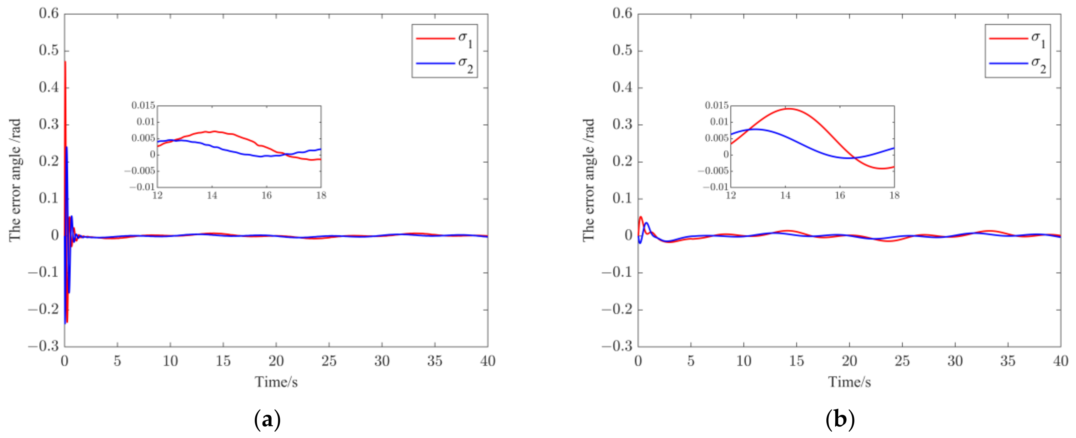
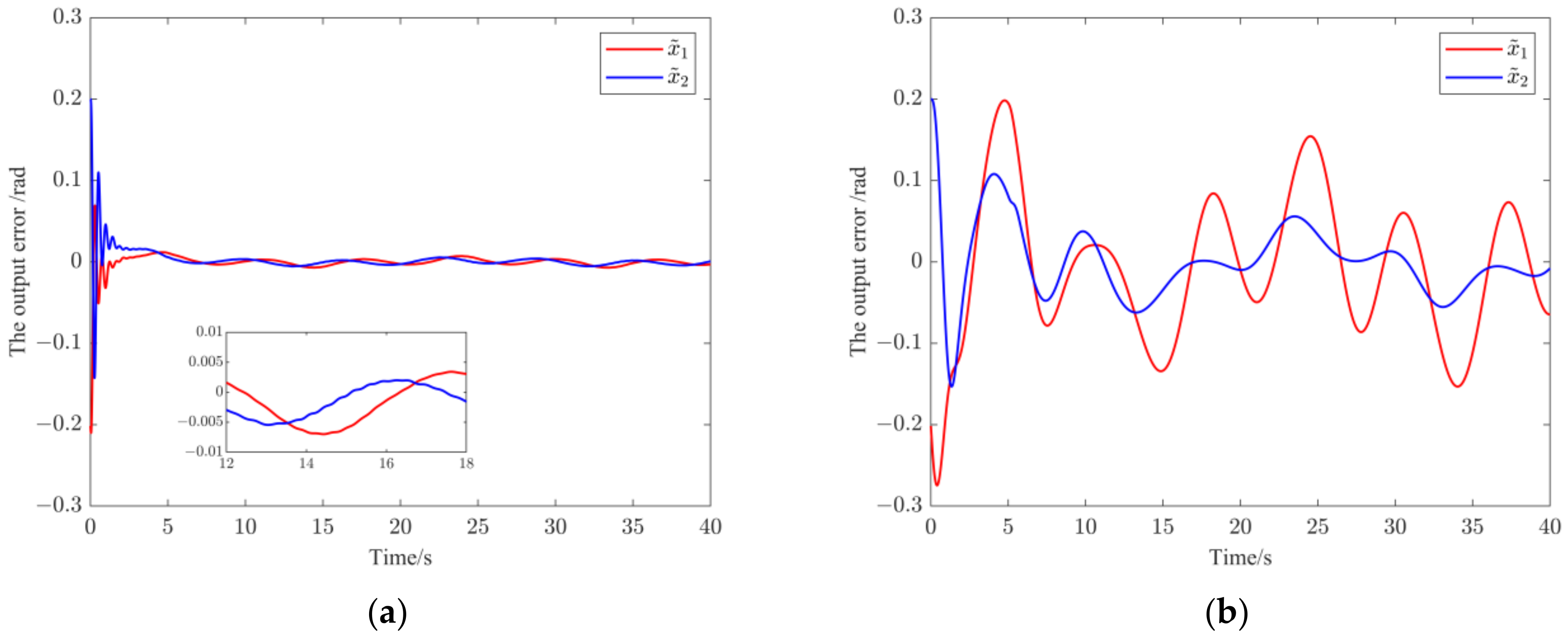
From Equation (8) we can see that when ε 0 , the flexible-joint’s stiffness coefficient matrix K θ . At this time, the connection between the motor rotor and the manipulator can be regarded as a rigid connection. θ = q θ , θ ˙ = q ˙ θ , θ ¨ = q ¨ θ , z θ = 0 . Let ε = 0 in Equations (9) and (10), and the slow subsystem’s dynamic equation can be obtained:
D θ s ( q ) q ¨ θ + C θ s ( q , q ˙ θ ) = ρ τ s + τ d
where, τ s R n × 1 is the slow subsystem’s controller. ρ = diag ( ρ 1 ρ i ρ n ) , ρ i ( 0 , 1 ] is actuator’s efficiency factor. D θ s ( q ) = D θ ( q ) + J θ , C θ s ( q , q ˙ θ ) is a new matrix by letting θ ˙ = q ˙ θ in C θ ( q , q ˙ θ , θ ˙ ) .
Firstly, we rewrite Equation (12) into the following form:
D θ s ( q ) q ¨ θ + H θ s ( q , q ˙ θ ) q ˙ θ = ρ τ s + τ d
The matrix in Equation (13) has the following properties:
Property 1 [40]: The inertial matrix D θ s ( q ) is symmetric positive definite and bounded. so 0 < ξ 1 y 1 2 y 1 T D θ s ( q ) y 1 ξ 2 y 1 2 , y 1 R n × 1 . Where, ξ 1 is the minimum eigenvalues of D θ s ( q ) , ξ 2 is the maximum eigenvalues of D θ s ( q ) .
Property 2 [41]: H θ s ( q , q ˙ θ ) R n × n can satisfy that: x T [ D ˙ θ s ( q ) 2 H θ s ( q , q ˙ θ ) ] x = 0 , x R n × 1 . Also H θ s ( q , q ˙ θ ) is bounded.
Property 3 [42]: for y 2 , y 3 , y 4 R n × 1 , there are: H θ s ( y 2 , y 3 ) ζ h y 3 , H θ s ( y 2 , y 3 ) y 4 = H θ s ( y 2 , y 4 ) y 3 . where, ζ h is a positive constant.
Property 4: τ d is bounded, and τ d ζ d , ζ d > 0 .
Defining state variables:
x 0 = q 0 ,   x 1 = q θ ,   x 2 = q ˙ θ
Thus, Equation (13)’s state-space form is:
x ˙ 1 = x 2 x ˙ 2 = D θ s 1 ( x 0 , x 1 ) [ ρ τ s + τ d H θ s ( x 0 , x 1 , x 2 ) x 2 ]
Let x ^ 1 be x 1 ’s estimated value, x ^ 2 be x 2 ’s estimated value. Then the link’s rotational angle error x ¯ 1 is:
x ¯ 1 = x 1 x ^ 1
And the link’s rotational angular velocity error x ¯ 2 is:
x ¯ 2 = x 2 x ^ 2
A velocity filter is designed for the slow subsystem:
x ^ ˙ 1 = x ^ 2 + K p x ¯ 1 + Λ 1 sgn ( x ¯ ) 1 x ^ ˙ 2 = D θ s 1 ( x 0 , x 1 ) [ ρ τ s H θ s ( x 0 , x 1 , x ^ 2 ) x ^ 2 ] + K v x ¯ 1 + Λ 2 sgn ( x ¯ ) 1
where, the matrix H θ s ( x 0 , x 1 , x ^ 2 ) is a new matrix gotten by letting x 2 = x ^ 2 in H θ s ( x 0 , x 1 , x 2 ) . K p and K v are positive definite diagonal matrices. Λ 1 = diag ( λ 1 , , λ i , , λ n ) , λ i is positive. Λ 2 ’s definition will be given below.
Subtracting Equations (15) and (18), we have:
x ¯ ˙ 1 = x ˙ 1 x ^ ˙ 1 = x ¯ 2 K p x ¯ 1 Λ 1 Sgn ( x ¯ ) 1 x ¯ ˙ 2 = x ˙ 2 x ^ ˙ 2 = D θ s 1 ( x 0 , x 1 ) [ H θ s ( x 0 , x 1 , x ^ 2 ) x ^ 2 H θ s ( x 0 , x 1 , x 2 ) x 2 + τ d ] K v x ¯ 1 Λ 2 Sgn ( x ¯ ) 1
Defining a sliding surface:
S = x ¯ 1
When the velocity filter’s the sliding mode occurs, that means x ¯ 1 = 0 and x ¯ ˙ 1 = 0 . Then from Equations (17) and (19), we have:
x ¯ ˙ 2 = D θ s 1 ( x 0 , x 1 ) [ H θ s ( x 0 , x 1 , x ^ 2 ) x ^ 2 + H θ s ( x 0 , x 1 , x 2 ) x 2 τ d ] Λ 2 Λ 1 1 x ¯ 2 = Λ 2 Λ 1 1 x ¯ 2 D θ s 1 ( x 0 , x 1 ) [ H θ s ( x 0 , x 1 , x ^ 2 ) x ¯ 2 + H θ s ( x 0 , x 1 , x 2 ) x 2 H θ s ( x 0 , x 1 , x ^ 2 ) x 2 τ d ]
According to property 3, there is:
H θ s ( x 0 , x 1 , x ^ 2 ) x 2 = H θ s ( x 0 , x 1 , x 2 ) x ^ 2
Thus, Equation (21) can be rewritten into the following form:
x ¯ ˙ 2 = Λ 2 Λ 1 1 x ¯ 2 D θ s 1 ( x 0 , x 1 ) [ H θ s ( x 0 , x 1 , x ^ 2 ) x ¯ 2 + H θ s ( x 0 , x 1 , x 2 ) x 2 H θ s ( x 0 , x 1 , x 2 ) x ^ 2 τ d ] = Λ 2 Λ 1 1 x ¯ 2 D θ s 1 ( x 0 , x 1 ) [ H θ s ( x 0 , x 1 , x ^ 2 ) x ¯ 2 + H θ s ( x 0 , x 1 , x 2 ) x ¯ 2 τ d ]
Then, the stability of the system needs to be proved. For nonlinear systems, we choose the Lyapunov function:
V = 1 2 x ¯ 2 T D θ s ( x 0 , x 1 ) x ¯ 2
We take the derivative of V with respect to time:
V ˙ = 1 2 x ¯ 2 T D ˙ θ s ( x 0 , x 1 ) x ¯ 2 + x ¯ 2 T D θ s ( x 0 , x 1 ) x ¯ ˙ 2
Substituting Equation (23) into Equation (25), we can obtain:
V ˙ = 1 2 x ¯ 2 T [ D ˙ θ s ( x 0 , x 1 ) 2 H θ s ( x 0 , x 1 , x 2 ) ] x ¯ 2 x ¯ 2 T D θ s ( x 0 , x 1 ) Λ 2 Λ 1 1 x ¯ 2 x ¯ 2 T H θ s ( x 0 , x 1 , x ^ 2 ) x ¯ 2 + x ¯ 2 T τ d
According to Properties 2, we have:
V ˙ = x ¯ 2 T D θ s ( x 0 , x 1 ) Λ 2 Λ 1 1 x ¯ 2 x ¯ 2 T H θ s ( x 0 , x 1 , x ^ 2 ) x ¯ 2 + x ¯ 2 T τ d
Let Λ 2 = D θ s 1 ( x 0 , x 1 ) [ K s H θ s ( x 0 , x 1 , x ^ 2 ) ] Λ 1 , where, K s R n × n . Then
V ˙ = x ¯ 2 T K s x ¯ 2 + x ¯ 2 T τ d = y T P y τ d T τ d
where, y = x ¯ 2 τ d , P = K s I / 2 I / 2 I .
Let K s = k s I , k s > 0 . From Equation (28) we can find that, when k s > 0.25 , P is a symmetric positive definite matrix, and λ min { P } < 1 . When k s , λ min { P } 1 .
Therefore, we have:
V ˙ λ min { Q } y 2 + τ d 2 x ¯ 2 + 2 ( 1 λ min { Q } λ min { Q } ) ζ d 2
From Equation (29) we can see that when the parameter k s is properly selected, the following equation is satisfied: when x ¯ 2 ζ d 1 λ min { Q } λ min { Q } = ζ 0 , V ˙ 0 . Otherwise, x ¯ 2 will converge to ζ 0 .
The backstepping method is a feasible controlling method for uncertain and nonlinear systems [43,44]. It is a step-by-step recursive design method: it can save the time for online calculation, and is more suitable for online control. This method combines the design of the control method with the choice of Lyapunov function and divides the system into several subsystems according to the design order. Firstly, a virtual controller and a Lyapunov function are designed for the lowest-order subsystem. Then continuing backstepping until the last subsystem. Finally, the control method is designed.
The slow subsystem’s desired output vector x 1 d and x 2 d are defined as:
x 1 d = q θ d = q 1 d q i d q n d T ,   x 2 d = q ˙ θ d = q ˙ 1 d q ˙ i d q ˙ n d T
where, q i d is q i ’s desired value, q ˙ i d is q ˙ i ’s desired value.
The output error vector x ˜ 1 is:
x ˜ 1 = x 1 d x 1
The velocity error vector x ˜ 2 is:
x ˜ 2 = x ˜ ˙ 1 = x 2 d x 2
The velocity estimation error vector x ˜ ^ 2 is:
x ˜ ^ 2 = x 2 d x ^ 2
Then, according to Equations (15), (31) and (32), the error equation is:
x ˜ ˙ 1 = x ˜ 2 x ˜ ˙ 2 = x ˙ 2 d D θ s 1 ( x 0 , x 1 ) [ ρ τ s + τ d H θ s ( x 0 , x 1 , x 2 ) x 2 ]
Step 1: Design for the system’s first-order variables.
Firstly, defining variables:
z 1 = x ˜ 1
and
z 2 = x ˜ 2 u z = z ˙ 1 u z
where, u z is a virtual controller. u z = A z 1 , A is a positive definite diagonal matrix.
Choosing the following Lyapunov function:
V 1 = 1 2 z 1 T z 1
Differentiating V 1 with respect to time, and according to Equation (36), there is:
V ˙ 1 = z 1 T z ˙ 1 = z 1 T ( z 2 + u z ) = z 1 T z 2 z 1 T A z 1
From Equation (38) we can find that, if and only when z 2 = 0 , V 1 is z 1 ’s quadratic function, and V ˙ 1 = z 1 T A z 1 0 . However, z 2 = 0 is a special case. So further design is needed.
Step 2: Based on Step 1, design for the second-order variables.
Selecting a new Lyapunov function to seek a control method to ensure that z 1 and z 2 can converge to zero. Firstly, from Equations (35) and (36), we have:
z 2 = x ˜ 2 + A x ˜ 1
and
z ˙ 2 = x ˜ ˙ 2 + A x ˜ ˙ 1
Substituting Equation (34) into Equation (40):
z ˙ 2 = x ˙ 2 d D θ s 1 ( x 0 , x 1 ) [ ρ τ s + τ d H θ s ( x 0 , x 1 , x 2 ) x 2 ] + A z ˙ 1
Defining a new Lyapunov function:
V 2 = 1 2 z 2 T D θ s ( x 0 , x 1 ) z 2
According to property 2, Equations (35), (39) and (41), V 2 ’s time derivative is:
V ˙ 2 = 1 2 z 2 T D ˙ θ s ( x 0 , x 1 ) z 2 + z 2 T D θ s ( x 0 , x 1 ) z ˙ 2 = z 2 T [ D θ s ( x 0 , x 1 ) ( x ˙ 2 d + A x ˜ 2 ) + H θ s ( x 0 , x 1 , x 2 ) ( x 2 d + A x ˜ 1 ) ρ τ s τ d ]
In practical application, the free-floating space robot system is often uncertain. Therefore, the matrix in Equation (13) should be exactly expressed as follows:
D θ s ( q ) = D ^ θ s ( q ) + Δ D θ s ( q ) ,   H θ s ( q , q ˙ θ ) = H ^ θ s ( q , q ˙ θ ) + Δ H θ s ( q , q ˙ θ )
where, D ^ θ s ( q ) is D θ s ( q ) ’s estimate matrix, H ^ θ s ( q , q ˙ θ ) is H θ s ( q , q ˙ θ ) ’s estimate matrix. Δ D θ s ( q ) and Δ H θ s ( q , q ˙ θ ) are the error. It is assumed that the system’s uncertain parameters are bounded. So, from Properties 1 and 2, we know that D θ s ( q ) and H θ s ( q , q ˙ θ ) are bounded. Therefore, D ^ θ s ( q ) , H ^ θ s ( q , q ˙ θ ) , Δ D θ s q and Δ H θ s q , q ˙ θ are also bounded.
We design a robust control law:
τ s = D ^ θ s ( x 0 , x 1 ) x ˙ 2 d + H ^ θ s ( x 0 , x 1 , x ^ 2 ) ( x 2 d + A x ˜ 1 ) + A B x ˜ 1 + [ D ^ θ s ( x 0 , x 1 ) A + B ] x ˜ ^ 2 + u
where, H ^ θ s ( x 0 , x 1 , x ^ 2 ) is a new matrix by letting x 2 = x ^ 2 in H ^ θ s ( x 0 , x 1 , x 2 ) . B is a positive definite diagonal matrix, u is a robust compensation controller for compensating the uncertainty of the system.
As can be seen from Equation (45), the control method does not include the speed variable x 2 of the system, so there is no need to measure the system’s speed in real time during the control process.
By substituting Equation (45) into Equation (44) and combining with Equations (32), (33) and (39), we have:
V ˙ 2 = z 2 T B z 2 + z 2 T ( η u )
where,
η = [ D θ s ( x 0 , x 1 ) D ^ θ s ( x 0 , x 1 ) ] ( x ˙ 2 d + A x ˜ ^ 2 ) [ D θ s ( x 0 , x 1 ) A + B ] x ¯ 2 + [ H θ s ( x 0 , x 1 , x 2 ) H ^ θ s ( x 0 , x 1 , x 2 ) ] ( x 2 d + A x ˜ 1 ) + τ d
Defining variable:
z ^ 2 = x ˜ ^ 2 + A x ˜ 1
Substituting Equations (17), (32), (33) and (39) into Equation (48), we have:
z ^ 2 = z 2 + x ¯ 2
Then, by substituting Equation (49) into Equation (46):
V ˙ 2 = z 2 T B z 2 + z ^ 2 T ( η u ) x ¯ 2 T ( η u )
Combining with Equations (14), (17), (33) and (48), we can rewrite Equation (47) as:
η = Δ D θ s ( x 0 , x 1 ) ( x ˙ 2 d + A x ˜ ^ 2 ) [ D θ s ( x 0 , x 1 ) A + B ] x ¯ 2 + [ Δ H θ s ( x 0 , x 1 , x 2 ) + H ^ θ s ( x 0 , x 1 , x ¯ 2 ) ] ( z ^ 2 + x ^ 2 ) + τ d
As we know,
η Δ D θ s ( x 0 , x 1 ) ( x ˙ 2 d + A x ˜ ^ 2 ) + D θ s ( x 0 , x 1 ) A + B x ¯ 2 + ( Δ H θ s ( x 0 , x 1 , x 2 ) + H ^ θ s ( x 0 , x 1 , x ¯ 2 ) ) ( z ^ 2 + x ^ 2 ) + τ d
According to property 2, property 3 and Equation (14), H ^ θ s ( x 0 , x 1 , x ¯ 2 ) is bounded. A and B are positive definite matrices, according to Property 1, D θ s ( x 0 , x 1 ) A + B is bounded. From the above analysis we know x ¯ 2 is bounded. According to Property 4, τ d is bounded. So η is bounded, η p , p is a positive constant.
The robust controller u is designed as following:
u = p z ^ 2 z ^ 2 z ^ 2 a p a z ^ 2 z ^ 2 < a
where, a is a positive constant.
According to Equations (50) and (53), when z ^ 2 = a 2 ,
V ˙ 2 λ min { B } z 2 2 + ( a 4 ζ 0 2 ) p
where, λ min { B } is the minimum of B ’s eigenvalue.
Obviously, when
z 2 p ( a 4 ζ 0 2 ) λ min { B }
, V ˙ 2 0 .
Because V 2 0 and V ˙ 2 0 , V 2 is bounded in t ( 0 , ) . Because V 2 is a function of z 2 , z 2 is bounded. z 2 = x ˜ 2 + A z 1 , z 1 = x ˜ 1 , and x ˜ 2 = x ˜ ˙ 1 , so x ˜ 2 , z 1 , z ˙ 1 , x ˜ 1 and x ˜ ˙ 1 are bounded. x ˜ 2 = q ˙ θ d x 2 , so x 2 is bounded. Then according to Equation (34), x ˜ ˙ 2 is bounded, z ˙ 2 = x ˜ ˙ 2 + A z ˙ 1 is also bounded. Therefore, according to Equation (43), V ˙ 2 is consistent and continuous in t ( 0 , ) . Because V 2 is bounded and V ˙ 2 0 , lim t V ˙ 2 = 0 . Because V ˙ 2 is a function of z 2 , lim t z 2 = 0 , and lim t x ˜ 1 = 0 , lim t x ˜ 2 = 0 . That is, the system is asymptotically stable. Otherwise, when Equation (55) is not satisfied, z 2 will converge to a small field near zero. At this time, the system’s tracking errors x ˜ 1 and x ˜ 2 are also consistent and ultimately bounded.
The block diagram of the control system is shown in Figure 3.

4. Simulation

We use the proposed robust backstepping fault-tolerant hybrid control (RBFTHC) to simulate the system shown in Figure 1. The parameters of the system are shown in Table 1. In the simulation, it is assumed that the load’s mass m p and the moment of inertia J p are uncertain parameters. The estimate values are: m ^ p = 1.5   kg , J p = 1   kg m 2 . The parameters of the control and simulation are shown in Table 2.
Simulation 1: The actuators work without fault, that is, ρ 1 = 1 , ρ 2 = 1 .
Case 1: Figure 4, Figure 5, Figure 6 and Figure 7 are the simulation results by using the proposed RBFTHC. The simulation results show that the system can achieve the asymptotic tracking of the joint desired motion trajectory accurately and stably. The output error x ˜ is very small (only from −6 to 3 × 10 3 rad), which reflects the excellent control precision of the system. The error angles caused by the flexible-joint are only from −1 to 7 × 10 3 rad, which indicates that the influence of the flexible-joints on the system is compensated, and that motion accuracy and stability of the system are achieved. The observation of the joint velocity based on the speed filter is also accurate, which reflects the validity and correctness of the proposed speed filter. In conclusion, the effectiveness of RBFTHC is verified.
Case 2: To prove the control effect of the robust controller u p in RBFTHC, we turn off u p . The simulation results are shown in Figure 8, Figure 9, Figure 10 and Figure 11. From the results we can find that when u p is off, the tracking accuracy of the joint angle’s desired trajectory is not good. The output error x ˜ becomes larger (from −116 to 70 × 10 3 rad) than the case of u p is on (from −6 to 3 × 10 3 rad). The system angle error σ becomes larger (from −5.8 to 10 × 10 3 rad) than the case of u p is on (from −1 to 7 × 10 3 rad). The observation of the joint velocity is not accurate. The reason for these results is that the uncertain parameters and the external disturbances of the system are not effectively compensated for. So, the simulation results prove that the proposed robust controller u p can compensate for the system’s uncertain parameters and external disturbances effectively.
Case 3: In order to verify the control effect of the fast subsystem’s controller τ f in RBFTHC, we turn off τ f . The simulation results are shown in Figure 12, Figure 13, Figure 14 and Figure 15. At this time, the system-elastic vibration caused by the flexible-joint is not suppressed, so the joint angle trajectories have seriously deviated from the expected trajectories in only 1.2 s. The output error and the angle error were large. So, the control failed. The effectiveness of the proposed fast subsystem controller τ f is verified. At the same time, the simulation results also prove that the strategy proposed in this paper, which uses a singular perturbation method to decompose the system and control the slow and fast subsystems separately, will be beneficial to the effective control of the strong rigid-flexible coupling system.
The comparison results of the three cases in Simulation 1 are shown in Table 3. It can also be seen from Table 3 that RBFTHC is effective and feasible. The robust controller u p and the fast subsystem’s controller τ f in RBFTHC can guarantee the accuracy and stability of the system effectively.
Simulation 2: The actuator is slightly faulty. The change of ρ is as follows:
ρ 1 = 1 0 < t 5 s 0.7 5 s < t 10 s 0.6 10 s < t 20 s ,   ρ 2 = 1 0 < t 4 s 0.6 4 s < t 12 s 0.5 12 s < t 20 s
In the simulation, we compare the control effect with the proposed RBFTHC and the computed torque control method (CTC) proposed by Angel and Viala [45], which does not consider the fault-tolerant control. The CTC is:
τ s = D θ s ( q ) q ¨ θ d K v x ˜ ˙ 1 K p x ˜ 1 + C θ s
The comparison simulation results are shown in Figure 16, Figure 17, Figure 18 and Figure 19. The numerical comparison results of x ˜ and σ under the two control methods are shown in Table 4. According to the results, we find that when actuator failure occurs, RBFTHC can still ensure that the system has good control quality. The motion trajectory of the joint angle of the system can still track the desired motion trajectory, and the vibration is suppressed. However, CTC has a poor trajectory-tracking effect. The output error x ˜ in CTC is 12 times larger than that in RBFTHC. The angle error σ in CTC is 2 times larger than that in RBFTHC.
Simulation 3: The actuator has a serious fault. The change of ρ is as follows:
ρ 1 = 1 0 < t 5 s 0.5 5 s < t 10 s 0.3 10 s < t 20 s ,   ρ 2 = 1 0 < t 4 s 0.4 4 s < t 12 s 0.3 12 s < t 20 s
The comparison simulation results are shown in Figure 20, Figure 21, Figure 22 and Figure 23. The numerical comparison results of x ˜ and σ under the two control methods are shown in Table 5. According to the results, we find that when an actuator has a serious fault, RBFTHC can also ensure that the system has good control quality. The motion trajectory of the joint angle of the system can still track the desired motion trajectory, and the vibration is suppressed. However, CTC cannot track the trajectory. The output error x ˜ in CTC is 35 times larger than that in RBFTHC. The angle error σ in CTC is three times larger than that in RBFTHC. The excellent fault tolerance performance of RBFTHC is proved.

5. Conclusions

We studied the control of free-floating flexible-joint space robots having uncertain parameters, external disturbance, and actuator faults. According to the singular perturbation method, the RBFTHC method consists of the slow subsystem’s robust backstepping fault-tolerant control, and the fast subsystem’s speed differential feedback control is proposed. The design process is evident, systematic, and structured. The RBFTHC method can reduce the flexible-joint angle error, compensate for the uncertain parameters and external interference, and realize the system’s joint angle trajectory tracking. The backstepping control makes the control system structure clear, the time of online calculation short, and does not require an uncertain system to meet the “matching condition”. The observer makes it inappropriate to measure and provide feedback on the system’s speed signal during the control process, so the control becomes simpler and more accurate. More importantly, when the actuator fails, the RBFTHC method can still ensure that the system maintains good control quality. It greatly improves the safety, reliability, maintainability, and service life of the space robot system. To the method has important practical significance and theoretical value.

Author Contributions

Conceptualization, L.X.; methodology, L.X. and X.Y.; software, L.X.; investigation, L.X. and X.Y.; writing—original draft preparation, L.X.; writing—review and editing, L.X. and X.Y.; supervision, L.X. and X.Y.; funding acquisition, L.X. and X.Y. All authors have read and agreed to the published version of the manuscript.

Funding

This research is supported by the National Natural Science Foundation of China (No. 51741502), the Natural Science Foundation of Fujian Province (No. 2020J01450) and the Education and Research Project for Young and Middle-aged Teachers of Fujian Provincial Department of Education (Science and Technology) (No. JAT210082).

Institutional Review Board Statement

Not applicable.

Informed Consent Statement

Informed consent was obtained from all subjects involved in the study.

Data Availability Statement

Not applicable.

Conflicts of Interest

The authors declare no conflict of interest.

References

  1. Shi, L.L.; Jayakoby, H.; Katupitiya, J.; Jin, X. Coordinated control of a dual-arm space robot. IEEE Robot. Autom. Mag. 2018, 25, 86–95. [Google Scholar] [CrossRef]
  2. Basmadji, F.L.; Seweryn, K.; Sasiadek, J.Z. Space robot motion planning in the presence of nonconserved linear and angular momenta. Multibody Syst. Dyn. 2020, 50, 71–96. [Google Scholar] [CrossRef]
  3. Zhou, Y.Q.; Luo, J.J.; Wang, M.M. Dynamic coupling analysis of multi-arm space robot. Acta Astronaut. 2019, 160, 583–593. [Google Scholar] [CrossRef]
  4. Kulakov, F.M. Methods of supervisory remote control over space robots. J. Comput. Syst. Sci. Int. 2018, 57, 822–839. [Google Scholar] [CrossRef]
  5. Zhao, S.P.; Siiciliano, B.; Zhu, Z.X.; Gutierrez-Giles, A.; Luo, J.J. Multi-waypoint-based path planning for free-floating space robots. Int. J. Robot. Autom. 2019, 34, 461–467. [Google Scholar] [CrossRef]
  6. Liu, X.F.; Zhang, X.Y.; Cai, G.P.; Chen, W.J. Capturing a space target using a flexible space robot. Appl. Sci. 2022, 12, 984. [Google Scholar] [CrossRef]
  7. Oda, M. Attitude control experiments of a robot satellite. J. Spacecr. Rocket. 2000, 37, 788–793. [Google Scholar] [CrossRef]
  8. Yu, X.Y. Augmented robust control of a free-floating flexible space robot. Proc. Inst. Mech. Eng. Part G-J. Aerosp. Eng. 2015, 229, 947–957. [Google Scholar] [CrossRef]
  9. Wang, G.; Shi, Z.C.; Shang, Y.; Sun, X.L.; Zhang, W.L.; Yu, Q.F. Precise monocular vision-based pose measurement system for lunar surface sampling manipulator. Sci. China-Technol. Sci. 2020, 62, 1783–1794. [Google Scholar] [CrossRef]
  10. Wei, J.; Cao, D.; Wang, L.; Huang, H.; Huang, W. Dynamic modeling and simulation for flexible spacecraft with flexible jointed solar panels. Int. J. Mech. Sci. 2017, 130, 558–570. [Google Scholar] [CrossRef]
  11. Ahmadi, S.; Fateh, M.M. Control of flexible joint robot manipulators by compensating flexibility. Iran. J. Fuzzy Syst. 2018, 15, 57–71. [Google Scholar]
  12. Meng, D.; She, Y.; Xu, W.; Lu, W.; Liang, B. Dynamic modeling and vibration characteristics analysis of flexible-link and flexible-joint space manipulator. Multibody Syst. Dyn. 2018, 43, 321–347. [Google Scholar] [CrossRef]
  13. Rsetam, K.; Cao, Z.; Man, Z. Cascaded extended state observer based sliding mode control for underactuated flexible joint robot. IEEE Trans. Ind. Electron. 2020, 67, 10822–10832. [Google Scholar] [CrossRef]
  14. Sun, W.; Su, S.F.; Xia, W.; Nguyen, V.T. Adaptive fuzzy tracking control of flexible-joint robots with full-state constraints. IEEE Trans. Syst. Man Cybern. -Syst. 2019, 49, 2201–2209. [Google Scholar] [CrossRef]
  15. He, W.; Yan, Z.C.; Sun, Y.K.; Ou, Y.S.; Sun, C.Y. Neural-learning-based control for a constrained robotic manipulator with flexible joints. IEEE Trans. Neural Netw. Learn. Syst. 2018, 29, 5993–6003. [Google Scholar] [CrossRef]
  16. Ling, S.; Wang, H.Q.; Liu, P.X. Adaptive fuzzy dynamic surface control of flexible-joint robot systems with input saturation. IEEE-CAA J. Autom. Sin. 2019, 6, 97–106. [Google Scholar] [CrossRef]
  17. Kim, J.; Croft, E.A. Full-state tracking control for flexible joint robots with singular perturbation techniques. IEEE Trans. Control Syst. Technol. 2019, 27, 63–73. [Google Scholar] [CrossRef]
  18. Ma, H.; Zhou, Q.; Li, H.Y.; Lu, R.Q. Adaptive prescribed performance control of a flexible-joint robotic manipulator with dynamic uncertainties. IEEE Trans. Cybern. 2022, 52, 12905–12915. [Google Scholar] [CrossRef]
  19. Diao, S.Z.; Sun, W.; Su, S.F.; Xia, J.W. Adaptive fuzzy event-triggered control for single-link flexible-joint robots with actuator failures. IEEE Trans. Cybern. 2021, 52, 7231–7241. [Google Scholar] [CrossRef]
  20. Zhang, D.G.; Angeles, J. Impact dynamics of flexible-joint robots. Comput. Struct. 2005, 83, 25–33. [Google Scholar] [CrossRef]
  21. Zhan, B.W.; Jin, M.H.; Liu, J. Extended-state-observer-based adaptive control of flexible-joint space manipulators with system uncertainties. Adv. Space Res. 2022, 69, 3088–3102. [Google Scholar] [CrossRef]
  22. Liu, L.X.; Hong, M.Q.; Gu, X.T.; Ding, M.; Guo, Y. Fixed-time anti-saturation compensators based impedance control with finite-time convergence for a free-flying flexible-joint space robot. Nonlinear Dyn. 2022, 109, 1671–1691. [Google Scholar] [CrossRef]
  23. Xie, L.M.; Yu, X.Y.; Chen, L. Robust fuzzy sliding mode control and vibration suppression of free-floating flexible-link and flexible-joints space manipulator with external interference and uncertain parameter. Robotica 2022, 40, 997–1019. [Google Scholar] [CrossRef]
  24. Liu, L.X.; Yao, W.; Guo, Y. Prescribed performance tracking control of a free-flying flexible-joint space robot with disturbances under input saturation. J. Frankl. Inst. -Eng. Appl. Math. 2021, 358, 4571–4601. [Google Scholar] [CrossRef]
  25. Chen, Z.; Li, Z. Dual-adaptive control of flexible-base flexible-joint space robot. J. Huazhong Univ. Sci. Technol. (Nat. Sci. Ed.) 2019, 47, 32–38. [Google Scholar]
  26. Le, Q.D.; Kang, H.J. Implementation of fault-tolerant control for a robot manipulator based on synchronous sliding mode control. Appl. Sci. 2020, 10, 2534. [Google Scholar] [CrossRef] [Green Version]
  27. Tan, N.; Zhong, Z.H.; Yu, P.; Li, Z.; Ni, F.L. A discrete model-free scheme for fault-tolerant tracking control of redundant manipulators. IEEE Trans. Ind. Inform. 2022, 18, 8595–8606. [Google Scholar] [CrossRef]
  28. Van, M.; Ceglarek, D. Robust fault tolerant control of robot manipulators with global fixed-time convergence. J. Frankl. Inst. -Eng. Appl. Math. 2021, 358, 699–722. [Google Scholar] [CrossRef]
  29. Lu, Z.P.; Li, Y.; Fan, X.R.; Li, Y.C. Decentralized fault tolerant control for modular robot manipulators via integral terminal sliding mode and disturbance observer. Int. J. Control Autom. Syst. 2022, 20, 3274–3284. [Google Scholar] [CrossRef]
  30. Liu, L.Z.; Zhang, L.Y.; Wang, Y.M.; Hou, Y.L. A novel robust fixed-time fault-tolerant tracking control of uncertain robot manipulators. IET Control Theory Appl. 2021, 15, 195–208. [Google Scholar] [CrossRef]
  31. Meng, Y.J.; Yang, H.; Jiang, B. Multi-model switching-based fault tolerant control for planar robot manipulators. IET Control Theory Appl. 2020, 14, 1–11. [Google Scholar] [CrossRef]
  32. Zhang, S.; Li, Y.Y.; Liu, S.; Shi, X.R.; Chai, H.; Cui, Y.G. A review on fault-tolerant control for robots. In Proceedings of the IEEE 2020 35th Youth Academic Annual Conference of Chinese Association of Automation (YAC), Zhanjiang, China, 16–18 October 2020; pp. 423–427. [Google Scholar]
  33. Wu, C.; Liu, J.; Xiong, Y.; Wu, L. Observer-based adaptive fault-tolerant tracking control of nonlinear nonstrict-feedback systems. IEEE Trans. Neural Netw. Learn. Syst. 2018, 29, 3022–3033. [Google Scholar] [CrossRef]
  34. Li, Y.X. Finite time command filtered adaptive fault tolerant control for a class of uncertain nonlinear systems. Automatica 2019, 106, 117–123. [Google Scholar] [CrossRef]
  35. Lei, R.H.; Chen, L. Adaptive fault-tolerant control based on boundary estimation for space robot under joint actuator faults and uncertain parameters. Def. Technol. 2019, 15, 964–971. [Google Scholar] [CrossRef]
  36. Yu, Z.W.; Cai, G.P. Dynamics modelling and fault tolerant control of 6-DOF space robot with flexible panels. Int. J. Robot. Autom. 2018, 33, 662–671. [Google Scholar]
  37. Lei, R.H.; Chen, L. Decentralized fault-tolerant control and vibration suppression for the elastic-base space robot with actuator faults and uncertain dynamics. J. Vib. Eng. Technol. 2021, 9, 2121–2131. [Google Scholar] [CrossRef]
  38. Lei, R.H.; Chen, L. Observer-based adaptive sliding mode fault-tolerant control for the underactuated space robot with joint actuator gain faults. Kybernetika 2021, 57, 160–173. [Google Scholar] [CrossRef]
  39. Spong M, W. Robot Dynamics and Control; John Wiley and Sons: New York, NY, USA, 1989. [Google Scholar]
  40. Lu, K.F.; Xia, Y.Q. Adaptive attitude tracking control for rigid spacecraft with finite-time convergence. Automatica 2013, 49, 3591–3599. [Google Scholar] [CrossRef]
  41. Chen, T.; Shan, J.; Wen, H. Distributed adaptive attitude control for networked underactuated flexible spacecraft. IEEE Trans. Aerosp. Electron. Syst. 2019, 55, 215–225. [Google Scholar] [CrossRef]
  42. Nicosia, S.; Tomei, P. Robot control by using only joint position measurements. IEEE Trans. Autom. Control 1990, 35, 1058–1061. [Google Scholar] [CrossRef]
  43. Cao, L.; Li, H.; Wang, N.; Zhou, Q. Observer-based event-triggered adaptive decentralized fuzzy control for nonlinear large-scale systems. IEEE Trans. Fuzzy Syst. 2019, 27, 1201–1214. [Google Scholar] [CrossRef]
  44. Li, Y.X.; Yang, G.H. Observer-based fuzzy adaptive event-triggered control co-design for a class of uncertain nonlinear systems. IEEE Trans. Fuzzy Syst. 2018, 26, 1589–1599. [Google Scholar] [CrossRef]
  45. Angel, L.; Viala, J. Tracking control for robotic manipulators using fractional order controllers with computed torque control. IEEE Lat. Am. Trans. 2018, 16, 1884–1891. [Google Scholar]
Figure 1. The simple model of joint. (a) The rigid-joint; (b) The flexible-joint.
Applsci 13 02634 g001
Figure 2. The free-floating flexible-joints space manipulator.
Applsci 13 02634 g002
Figure 3. The control system.
Applsci 13 02634 g003
Figure 4. The trajectories of the joint angle q θ .
Applsci 13 02634 g004
Figure 5. The output error x ˜ .
Applsci 13 02634 g005
Figure 6. The angle error σ .
Applsci 13 02634 g006
Figure 7. The joint angular velocity q ˙ θ .
Applsci 13 02634 g007
Figure 8. The trajectories of the joint angle q θ when u p is off.
Applsci 13 02634 g008
Figure 9. The output error x ˜ when u p is off.
Applsci 13 02634 g009
Figure 10. The angle error σ when u p is off.
Applsci 13 02634 g010
Figure 11. The joint angular velocity q ˙ θ when u p is off.
Applsci 13 02634 g011
Figure 12. The trajectories of the joint angle q θ when τ f is off.
Applsci 13 02634 g012
Figure 13. The output error x ˜ when τ f is off.
Applsci 13 02634 g013
Figure 14. The angle error σ when τ f is off.
Applsci 13 02634 g014
Figure 15. The joint angular velocity q ˙ θ when τ f is off.
Applsci 13 02634 g015
Figure 16. The trajectories of the joint angle q θ (a) RBFTHC, (b) CTC.
Applsci 13 02634 g016
Figure 17. The output error x ˜ . (a) RBFTHC, (b) CTC.
Applsci 13 02634 g017
Figure 18. The angle error σ . (a) RBFTHC, (b) CTC.
Applsci 13 02634 g018
Figure 19. The joint angular velocity q ˙ θ . (a) RBFTHC, (b) CTC.
Applsci 13 02634 g019
Figure 20. The trajectories of the joint angle q θ . (a) RBFTHC, (b) CTC.
Applsci 13 02634 g020
Figure 21. The output error x ˜ . (a) RBFTHC, (b) CTC.
Applsci 13 02634 g021
Figure 22. The angle error σ . (a) RBFTHC, (b) CTC.
Applsci 13 02634 g022
Figure 23. The joint angular velocity q ˙ θ . (a) RBFTHC, (b) CTC.
Applsci 13 02634 g023
Table 1. The parameters of the system.
BodyMass
(kg)
Length (m)Moment of Inertia
( kg m 2 )
Stiffness Coefficient ( N m / rad )
base401.534.17
Link B 1 231.5
Link B 2 130.75
Motor rotor000.5100
loaduncertain uncertain
Table 2. The parameters of the control.
The control parameters Λ 1 = d i a g ( 0.1 , 0.1 ) ,   K p = d i a g ( 50 , 50 ) ,   K v = d i a g ( 10 , 10 ) ,   K s = d i a g ( 10 , 10 ) ,   A = d i a g ( 30 , 30 ) ,   B = d i a g ( 100 , 100 ) ,   a = 0.05 ,   p = 5 + 0.1 z ^ 2
The desired trajectories q 1 d = sin π 10 t , q 2 d = c o s π 10 t
The system initial values q ( 0 ) = [ 1.9 0.1 1.5 ] T r a d , θ ( 0 ) = [ 0.1 1.5 ] T r a d
The external disturbance τ d = [ sin ( t ) cos ( t ) ] T N m
The simulation time t = 40 s
Table 3. The simulation results.
The   Output   Error   x ˜ ( × 10 3 rad ) The   Angle   Error   σ ( × 10 3 rad )
RBFTHC−4.6~5.1−4.6~5.8
u p is off−100~80−10~10
τ f is off
Table 4. The simulation 2 results.
The   Output   Error   x ˜ ( × 10 3 rad ) The   Angle   Error   σ ( × 10 3 rad )
RBFTHC−6~3−1.5~7
CTC−46~63−4~14
Table 5. The simulation 3 results.
The   Output   Error   x ˜ ( × 10 3 rad ) The   Angle   Error   σ ( × 10 3 rad )
RBFTHC−7~3−1.5~7
CTC−153~198−9~16
Disclaimer/Publisher’s Note: The statements, opinions and data contained in all publications are solely those of the individual author(s) and contributor(s) and not of MDPI and/or the editor(s). MDPI and/or the editor(s) disclaim responsibility for any injury to people or property resulting from any ideas, methods, instructions or products referred to in the content.

