Evaluating Deep Learning Techniques for Natural Language Inference

Abstract

Natural language inference (NLI) is one of the most important natural language understanding (NLU) tasks. NLI expresses the ability to infer information during spoken or written communication. The NLI task concerns the determination of the entailment relation of a pair of sentences, called the premise and hypothesis. If the premise entails the hypothesis, the pair is labeled as an “entailment”. If the hypothesis contradicts the premise, the pair is labeled a “contradiction”, and if there is not enough information to infer a relationship, the pair is labeled as “neutral”. In this paper, we present experimentation results of using modern deep learning (DL) models, such as the pre-trained transformer BERT, as well as additional models that relay on LSTM networks, for the NLI task. We compare five DL models (and variations of them) on eight widely used NLI datasets. We trained and fine-tuned the hyperparameters for each model to achieve the best performance for each dataset, where we achieved some state-of-the-art results. Next, we examined the inference ability of the models on the BreakingNLI dataset, which evaluates the model’s ability to recognize lexical inferences. Finally, we tested the generalization power of our models across all the NLI datasets. The results of the study are quite interesting. In the first part of our experimentation, the results indicate the performance advantage of the pre-trained transformers BERT, RoBERTa, and ALBERT over other deep learning models. This became more evident when they were tested on the BreakingNLI dataset. We also see a pattern of improved performance when the larger models are used. However, ALBERT, given that it has 18 times fewer parameters, achieved quite remarkable performance.

1. Introduction

During human communication, a lot of information is conveyed. Usually, the receiver gains a lot more information than what is uttered by the speaker. This is due to the natural inference capabilities of humans or general world knowledge. For example, the sentence “John grew up in Spain” gives a lot more information than simply the birthplace of John. We can assume that John speaks Spanish, and he went to school in Spain. Additionally, we can assume that John adopts the Spanish culture and therefore likes or plays football; furthermore, he likes Spanish food. All this information is taken for granted when we talk to each other, but to a computer, much more work needs to be done to feed this extra information. This is what natural language inference (NLI) deals with, and this is why, from its beginning, NLI was thought to be necessary for full natural language understanding [1].

Natural language inference is the task of determining the entailment relation between a premise and its hypothesis. This relation is usually described with one of three labels: entailment, contradiction, or neutral. An NLI sentence pair is classified as entailment if, given its premise, a human would be happy to infer the hypothesis. If the hypothesis directly contradicts the premise, the pair is labeled as a contradiction. In the case where not enough information is present to label a pair as entailment or contradiction, the ‘neutral’ label is annotated. In some datasets, the problem is set as a 2-label classification task, with one of the labels being ‘entailment’ and the other ‘not entailment’. The definition of “a human being happy to infer the hypothesis” may seem vague, but it has to be, given that the language itself is complicated, and many times, the same sentence can have different meanings to different people. In this line, it is well stated that the sentence pairs should be annotated by people that are awake, careful, moderately intelligent and informed [2].

In

Table 1. Examples of NLI sentence pairs and their label.

Premise	Hypothesis	Label
A soccer game with multiple males playing	Some men are playing a sport	Entailment
The girl went out wearing a costume	The girl went out wearing a fairy costume	Neutral
A boat sank in the Pacific Ocean	A boat sank in the Atlantic Ocean	Contradiction

, three examples of sentence pairs for NLI and the resulting labels are presented. The premise is the first sentence, which provides us with the context to be used. The hypothesis is the second sentence, in which we will be asked whether it can be inferred from the premise. The label describes the entailment relationship of the two sentences. Given the first example in Table 1, we see that the correct label is entailment because, by reading the premise, we can safely infer that the hypothesis is also true. The next example, however, is not an entailment, as the hypothesis adds information that is not present in the premise. We cannot safely say that the costume the girl is wearing is indeed a fairy costume, as it could be any type of costume. On the other hand, we do not have information that says that the costume is not a fairy costume; therefore, the correct label for this pair is neutral. In the last case, the first thought is that the pair should be labeled as a contradiction since we are talking about two different oceans. However, one could say that a boat sinking in the Pacific Ocean does not negate a boat sinking in the Atlantic Ocean, meaning that both sentences could be true. To avoid such conflictions, we always consider that we are talking about one single event. Therefore, the correct label is contradiction.

The NLI task needs special handling and has posed great challenges to the NLP research community since its formulation in 2005 with the recognizing textual entailment (RTE) challenges [3]. Since then, a lot of progress has been made both in terms of available data, as well as in the development of models that try to face the NLI problem. In 2015, the first large-scale NLI dataset was collected and provided neural models with 550,000 examples of crowdsource-labeled data [4]. These assisted in gaining more attention to the field of NLI, which brought many advances but also many criticisms. In 2017, the GLUE benchmark for natural language understanding [5] was published, which includes four NLI task datasets (MNLI, QNLI, RTE, WNLI). The collection method of each dataset is different, and so each dataset evaluates a different type of inference ability. This benchmark later evolved into SuperGLUE [6], which includes even harder and more challenging tasks.

As already stated, the main type of inference models today are deep neural network models. Up to 2017, the dominant type of inference model consisted of LSTMs (a deep learning model) encoding the premise and hypothesis, then applying an attention mechanism before passing the final vector to a SoftMax function for classification. A model that fits in this description is ESIM [7], which at that time demonstrated a state-of-the-art 88.0% accuracy on the SNLI dataset. Later adaptations of such models included additional learning from a knowledge graph to incorporate external world knowledge into the model [8]. Recently, the invention of transformers [9] and, more specifically, BERT [10] has switched research to using pre-trained models on large corpora of text that are then fine-tuned on specific data. Such models (ΒΕRT, XLNet, RoBERTa, ALBERT) quickly became the state-of-the-art models for NLI, performing with over 90% accuracy on some of the most challenging datasets.

However, many researchers questioned the ability of these models’ inference abilities as they argued that the models take advantage of various annotation artifacts within the datasets to achieve their results. One of the first papers that addressed this issue was Poliak et al.’s hypothesis-only approach [11]. In their paper, they showed that only using the hypothesis sentence for some NLI datasets performed well above random chance, suggesting that specific words in the hypotheses are related to a specific label. Furthermore, some studies [12] found instances of social bias in the examples of the SNLI dataset, while others [13] found wrong labels in the SICK dataset as well. To continue testing that idea, some researchers developed NLI stress tests to break top-performing NLI models, such as the BreakingNLI dataset [14]. Furthermore, additional adversarial datasets were developed with a focus on collecting examples that top-performing models predict wrong [15].

The protocol of collecting annotations for sentence pairs has been criticized by researchers in the field as not satisfactory [16,17]. The idea behind the criticisms is that one should not take the label most voted on by humans as the gold label and should not ignore other opinions. Pavlick et al. [18] believe that NLI needs a revision because the vague task of “do as a human would” is not in agreement with the fact that different humans can extract different conclusions from the same sentence pair. Therefore, they suggested a new type of measurement that takes into account the entire spectrum of opinions. One such dataset is ChaosNLI [17], which instead of gold labels, uses a distribution over a collective of human opinions.

Another way of improving NLI is by creating new and more diverse datasets that cover a quite broad range of linguistic phenomena. An example in this direction is the IMPLI dataset [19], which uses sentence pairs of figurative language and tests models on idiomatic expressions and metaphors. Another dataset is ANLI, which uses adversarial data to trick NLI models. However, some researchers argue that models could be implemented to purposely exploit such data for better scores [20]. One recent approach to creating datasets for NLI is WANLI [21], which takes advantage of the progress of natural language generation models to include them in the process of data creation together with human annotators. Additionally, human explanations of data have been used in the training process, with the aim of improving NLI, with good results [22].

We are not interested in a model that performs exceptionally well in a specific task; rather, we are looking for a model that genuinely learns to infer information and can do so using different datasets. One way to test this ability is by generalizing knowledge from one task to another, which is the main objective of this work. In this paper, we experiment with five (5) modern deep learning models plus their variations on eight (8) popular benchmarks for NLI. The models can be distinguished into two categories: traditional deep learning models with attention mechanisms and modern transformer-based models. In the first category, we deal with the decomposable attention model (DAM) [23], which is a model that uses attention without LSTMs, and ESIM, which is a model that uses chain LSTMs with an attention mechanism. The second category of models comprises three BERT implementations: BERT, RoBERTa [24], and ALBERT [25]. These models are pre-trained on large corpora of text data. We also present and use eight popular NLI datasets: MNLI [26], QNLI, RTE, WNLI (all four belonging to the GLUE Benchmark), SNLI, SciTail [27], SICK [28], and DNLI [29].

For each model and dataset combination, we explore a wide range of hyperparameters. We compare the best accuracies on the test or development set. Next, we test our models on BreakingNLI, a dataset that evaluates models’ inference ability, which requires basic lexical and world knowledge. For this experiment, we train the models on SNLI and MNLI training data. Finally, we conduct generalization ability tests such as Talman’s and Chatzikyriakidis’s tests [30], where we train each model on a dataset but test its predictions on test data from the other datasets. This experiment tests whether the inference ability of models can be transferred across NLI datasets.

We show that BERT models very clearly outperform the old-generation models on all NLI benchmarks. Furthermore, between the BERT models, we see an improvement in accuracy when using the larger version, although ALBERT shows a comparative performance with 18 times fewer parameters. In the attempt to “break” our models with the BreakingNLI test set, we see that the pre-trained transformers keep their high scores in contrast to the other models. However, the BERT models fail on the generalization test as the accuracy drops significantly when the datasets are not similar enough, which is in line with findings in the literature [30].

The main contributions of this paper are:

• Configuration of new state-of-the-art deep learning models for the NLI problem.
• Extensive evaluation of the models on the most widely used datasets.
• Extensive evaluation of the generalization ability of the models.

The rest of the paper is organized as follows. Section 2 presents a literature review of the deep learning methods for solving the NLI problem. In Section 3, our methodology is described, whereas in Section 4, the datasets used are described. Section 5 presents the experimental results, while Section 6 deals with the evaluation of the generalization capabilities of the models. Finally, Section 7 concludes the paper.

2. Related Work

One of the first attempts at NLI was the decomposable attention model (DAM) [23]. The authors of the DAM presented an attention model for NLI that decomposes the problem into sub-problems that can be parallelized. The model works in three steps: attend, compare, and aggregate. In the first step, the premise and the hypothesis are encoded to two vectors, a and b, and then an attention mechanism is applied between them. The attention mechanism finds the sub-phrases in b that are softly aligned with every word in a, as well as the sub-phrases in a that are aligned with every word in b. In the second step, the words of a and their aligned sub-phrases in b are compared with a feed-forward neural network and are passed in a vector, the same as b. In the third step, the values in each vector are aggregated and passed to a final MLP with SoftMax for classification. In addition to the three steps, an optional attention step was presented, called intra-sentence attention. This step can take place before the attend step, and it calculates the self-attention of a sentence for better representation. The DAM was trained on the SNLI dataset with GloVe embeddings. It provided state-of-the-art results at that time: 86.3% on the test set for the basic steps and 86.8% with the inclusion of the intra-attention step.

Another popular model is enhanced sequential inference modeling (ESIM) [7]. The authors of ESIM focus on enhancing sequential models for inference. Their model is based on chaining LSTMs and applying attention mechanisms. In their paper, they also present a tree-LSTM model that encodes syntactic knowledge and can be used together with ESIM to form HIM (hybrid inference model). ESIM also works in three steps, similar to DAM: input encoding, local inference modeling and inference composition. In the first step, the premise and hypothesis are encoded with bidirectional LSTMs. The outputs of the biLSTMs are combined with an attention mechanism. The resulting vectors (the softly aligned representations of a and b) and the original vectors a and b are then further combined and concatenated for better representation. In the third step, the outputs of the second step are again fed into two biLSTMs. Then, instead of aggregating the resulting vectors, they compute the average and max pooling of both vectors, and the four resulting vectors are concatenated and fed in an MLP with a SoftMax for classification. The authors trained the model on SNLI with 300d GloVe embeddings with a batch size of 32, using the Adam optimizer with a learning rate of 0.0004 and a dropout rate of 0.5. The model provided the best result at that time on the SNLI test set (88.00%).

The invention of transformers bred a new generation of models for NLI. The first popular adaptation was BERT (bidirectional encoding representations from transformers) [10]. BERT is a bidirectional language representation model that uses the architecture of the transformer model, more specifically, the encoder part of the transformer model. BERT is pre-trained on large corpora of unlabeled text that can then be fine-tuned on specific data. During pre-training, BERT performs two tasks: masked language modeling (MLM) and next-sentence prediction (NSP). MLM is essentially how BERT manages to learn in a bidirectional manner. The task of MLM includes masking a percentage of the input at random and then trying to figure out the correct word given its context (the words to the left and right of the mask). In the NSP task, BERT is given two sentences and must predict if one sentence (logically) follows the other. Due to its similarity, NSP is supposed to help with performance on NLI tasks. BERT is trained on the BookCorpus and the English Wikipedia (800 M + 2.5 B words). The input of BERT is a sequence of a maximum of 512 tokens. The first token is always the special (CLS) token, which encodes the classification, and sentences in the input are separated with the special (SEP) token. BERT uses WordPiece embeddings with a vocabulary of 30,000 words. In addition to token embeddings, BERT uses segment embedding, which matches a token with the sentence it appears in, and positional embedding, which tracks the position of the embeddings. There are two BERT sizes available: BERT-Base (110 M params) and BERT-Large (345 M params). BERT has demonstrated new state-of-the-art results on many NLP tasks, including NLI.

Another popular transformer model is RoBERTa (Robustly Optimized BERT Approach) [24]. The authors of RoBERTa believed that BERT was undertrained, so they presented a more optimized approach to training BERT called RoBERTa. The main changes regard the hyperparameters of pre-training, the task of MLM, the removal of the NSP task and the usage of more pre-training data. RoBERTa was trained on BookCorpus, Wikipedia, CC-NEWS, OPENWEBTEXT, and STORIES, totaling 148 GB of uncompressed text. The change in the MLM tasks is the introduction of dynamic masking, which creates a new masking pattern for each input sequence. In addition to dynamic masking, training data are replicated 10 times so that many masking patterns are created. They removed the NSP loss after carrying out several experiments that showed that NSP hurts performance. Finally, they used Byte-Pair Encoding, which encodes bytes instead of Unicode characters, resulting in a larger vocabulary of 50,000 words. As with BERT, RoBERTa comes in two sizes: Base and Large. RoBERTa-Base is comprised of L = 12 layers, a hidden size of H = 768, and A = 12 attention heads (110 M params). RoBERTa-Large has 355 M parameters (L = 24, H = 1024, A = 16) and has demonstrated state-of-the-art results on many NLP tasks, surpassing BERT.

A problem with BERT and ROBERTA is that they have hundreds of millions of parameters. This puts many restrictions on the training process as it requires a lot of GPU memory and is very time-consuming. Researchers from Google Research and Toyota Technological Institute in Chicago developed a different version of BERT called ALBERT (A Lite BERT) [25]. ALBERT is a light version of BERT that uses significantly fewer parameters. ALBERT uses the same architecture as BERT but makes three important distinctions. First, the vocabulary embedding is decomposed into two smaller ones. Second, parameters are shared across all layers, and third, NSP is replaced by a sentence-order prediction task. In BERT and RoBERTa, the embedding size is tied with the hidden size, E = H. The authors believe this is suboptimal, as H encodes context-depended information and E encodes context-independent information; thus, H should be bigger than E, H >> E. Therefore, instead of projecting the one-hot vectors onto H, they first project them on a smaller matrix, E, and then E is projected onto H. This way, the parameters are reduced from O (V × H) to O (V × E + E × H), which is critical when H >> E. Next, parameter sharing is used as it provides a smoother change from layer to layer. Lastly, NSP was replaced by SOP, a task that focuses on inter-sentence coherence. SOP gives positive feedback when one sentence follows the other but negative when the same two sentences are inserted with their order switched. There are four versions of ALBERT: base, large, xlarge, and xxlarge. They have 11, 17, 60, and 235 million parameters, respectively. ALBERT’s xxlarge version has demonstrated new state-of-the-art results, surpassing RoBERTa on several NLI tasks.

A more recent approach is ERNIE 3.0 [31], developed by researchers at Baidu. The authors saw a problem with the data used for training in popular models. They believed that the text used was plain and did not incorporate linguistic and word knowledge. Another problem they found was that the models were trained in an auto-regressive way, which, according to J. Devlin et al., worsens performance on downstream tasks [6]. Their proposal, ERNIE, is a unified framework to train large-scale models on a big corpus of text data as well as a knowledge graph. ERNIE combines the auto-regressive network and auto-encoding network so that both NLU and NLG are achieved. The model was tested on many Chinese NLP tasks and achieved first place on the SuperGLUE benchmark. ERNIE uses a shared network as the backbone to capture universal lexical and syntactic information, which is called the universal representation module, and it is built with a multi-layer Transformer-XL. ERNIE also uses a task-specific representation module, which is also a multi-layer transformer XL that is used to capture the top-level semantic representation for different task paradigms. While pre-training ERNIE, the authors used several pre-training tasks. The two word-aware tasks were knowledge-masked language modeling and document language modeling. The first masks phrases and named entities for the model to predict. The second is a pre-training task in which a traditional language model is used for generative purposes. Two structure-aware tasks were used: sentence reordering, in which the model tries to recreate a sentence given the segments of the sentence in random order, and sentence distance, which is an extension of the NSP task. The final task used was the universal knowledge-text prediction task. This task requires unstructured text and knowledge graphs. The way it works is, given a triple from the graph and a sentence from an encyclopedia, the model tries to predict the relation in the triple from the sentence. ERNIE 3.0 was tested on Chinese versions of NLI datasets and demonstrated new state-of-the-art results on OCLI and XNLI. In more detail, ERNIE demonstrated 82.75% accuracy on the OCNLI development set compared to the previous 78.80% accuracy exhibited by RoBERTa. On XNLI, the accuracy achieved on the test set was 83.77%, which is a smaller increase from the former best accuracy of 83.09%.

The pathways language model (PaLM) is a recent contribution to NLU and NLG developed by engineers at Google [32]. It is a 540 billion parameter language model based on a transformer trained on 6144 TPU v4 chips. It brought impressive results with few-shot learning as well as with fine-tuning specific NLP tasks. PaLM uses the transformer architecture, using only the decoder and some additional architectural differences. The authors preferred swiGLU activation functions over ReLU for the MLP. They also used a different formulation in each transformer block for faster training speeds at large scales. They used RoPE embeddings, shared input-output embeddings and a SentencePiece vocabulary with 256 k tokens. The model was pre-trained on 780 billion tokens. The data were taken from filtered webpages, books, Wikipedia, news articles, source code and social media conversations, which comprise 50% of the total data. They created three versions of the model: an 8 B parameter model with 32 layers, 16 attention heads, and a hidden layer size of 4096; a 62 B parameter model with 64 layers, 32 attention heads, and a hidden layer size of 8192; and finally, a 540 B parameter model with 118 layers, 48 attention heads and a hidden layer size of 18,432. The model was evaluated on 29 benchmarks, including SuperGlUE and ANLI. After being fine-tuned on SuperGLUE, the model performed close to SOTA results, and it currently stands 3rd on the leaderboard. On ANLI, the largest model exhibits 56.9% accuracy with few-shot learning.

ST-MoE (stable and transferable mixture-of-experts) is a recent approach to tackle NLU [33]. Developed by researchers at Google Brain, it is a 269-billion-parameter sparse model that manages to achieve state-of-the-art results in many NLP tasks. One of its main advantages is that it avoids the usual training instabilities often encountered in sparse models. Training instability was the main focus of work in the paper, and the authors tried to tackle it from many angles. They proposed a new type of loss called router z-loss, which they found to improve stability without degrading the quality of the model. They followed the traditional approach of pre-training on large data and fine-tuning downstream tasks. In the fine-tuning phase, they noticed overfitting issues on two SuperGLUE tasks. To answer this problem, they updated only a subset of model parameters during fine-tuning. The model was tested on many NLU tasks, including several NLI tasks. On RTE, the model demonstrates 93.5% accuracy, and on the R3 test set of ANLI, it exhibits an impressive 74.7% accuracy. The model currently holds first place on the leaderboard of the SuperGlue benchmark.

3. Methodology

We configured and trained 5 DL models, DAM, ESIM, BERT, RoBERTa, and ALBERT, along with their variations, on the 8 most popular datasets (presented in the next section). We tuned the hyperparameters for each model and task to achieve the best accuracies. Next, we tested our model’s inference ability on the Breaking NLI dataset when trained on SNLI or MNLI. Finally, we carried out a generalization experiment with the 5 state-of-the-art models and the 8 datasets (4 three-way classifications and 4 two-way classifications).

For DAM, we used both the vanilla version as well as the version with the intra-sentence attention. For the DAM implementations, we chose our hyperparameters starting from the recommended ones in the original paper. The values we tried were a batch size of {16, 32, 64}, hidden layer size of {100, 200, 300}, the AdaGrad optimizer with a learning rate of {0.05, 0.025, 0.01}, a dropout rate of {0.2, 0.5}, and a weight decay of {10⁻⁵, 10⁻⁴}. We used 300-dimensional GloVe embeddings, which remained fixed during training. We trained the model with an early stopping patience value depending on each dataset. The GluonNLP implementations demonstrated 85.0% accuracy on SNLI, which is 1.3% lower than the original paper.

We trained ESIM starting from the hyperparameters of the original paper. In our experiments, we tried the following values: a batch size of {16, 32, 64}, a hidden layer size of {100, 200, 300}, the Adam optimizer with a learning rate of {0.0001, 0.0004, 0.0005}, a dropout rate of {0.5, 0.8}, and a weight decay of {10⁻⁵, 10⁻⁴}. Similarly, with DAM, we used 300d GloVe embeddings and early stopping for training.

We trained BERT (Base/Large) and RoBERTa (Base/Large) models on all datasets. On the GLUE datasets (MNLI, QNLI, RTE, WNLI), we used the GluonNLP toolkit and tried the following hyperparameters for BERT-Base: a batch size of {16, 32, 64}, a learning rate of {10⁻⁵, 10⁻⁴, 2 × 10⁻⁵, 3 × 10⁻⁵, 4 × 10⁻⁵, 5 × 10⁻⁵, 5 × 10⁻⁶}, a warmup ratio of {0.05, 0.1, 0.2}, and {4} epochs. For the Large versions, we were restricted to using a batch size of 16 due to GPU memory limitations on Kaggle. Especially for the MNLI dataset, we trained it for 3 epochs due to Kaggle time restrictions. For the other 4 datasets, we used a different toolkit: JiantNLP. We still trained the models with the same batch sizes and learning rates; however, we performed validation tests more often on a subset (500 samples) of the valuation set. Furthermore, we performed early stopping on the accuracies of these subsets. Therefore, the training process was quicker without losing on performance. In the gluonNLP experiments, the max input sequence was set to 128, and on JiantNLP, it was set to 256. In all the experiments, we used the AdamW optimizer with an epsilon of 10⁻⁶.

We used JiantNLP for all the experiments with ALBERT (max input sequence was set to 256). We used the base and the large versions of ALBERT, which are significantly smaller than the BERT and Roberta equivalents. We tried the same hyperparameters with the addition of using a bigger batch size with the large version, as its smaller size allows it. The rest of the details are the same as the previous experiments with Jiant.

4. Datasets

The datasets we used in our experiments can be distinguished into two main categories according to the number of labels they consist of. We used 4 datasets with 3-way classification (SNLI, MNLI, SICK, and DNLI) and 4 with 2-way classification (QNLI, RTE, WNLI, and SciTail). Moreover, we performed some experiments on the BreakingNLI test set, which uses three labels.

The Stanford NLI dataset (SNLI) [4] is the largest collection of NLI data, consisting of 570,000 examples. Its premises are captions of photos from the Flickr30k dataset. The hypotheses were written by human workers through Amazon’s Mechanical Turk. The workers were asked to write three hypotheses for one premise (one for each label), and then the sentence pair was given to other workers for further labeling. The label with the most votes (out of 5) became the gold label for the pair. SNLI was split to train/dev/test sets, which contained 550,000, 10,000, and 10,000 examples, respectively. As for the labels (entailment, contradiction, neutral), they were equally distributed across the dataset.

The Multi-Genre NLI dataset (MNLI) [26] was created with the goal of being a better benchmark for NLU. It is comparable in size to SNLI as it consists of 433,000 examples. MNLI, in contrast to SNLI, contains many types of examples and not just one (photo captions). The collection process was similar to that of SNLI (AMT, gold labels). The distinct characteristic of MNLI is that it contains examples from 10 different sources of text. The 10 categories are: FACE-TO-FACE (transcriptions), GOVERNMENT (reports, speeches), LETTERS, 9/11 (reports on terrorist attacks), non-fiction works OUP, popular culture articles SLATE, TELEPHONE (phone conversations), TRAVEL (travel guides), VERBATIM (essays on linguistics), and FICTION (fiction novels). The MNLI dataset is split into a training set, 2 development sets, and 2 test sets. The training set, together with the matched development/test sets, includes 5 of the 10 categories, while the mismatched development and testing sets include the other 5 categories. The training set consists of 390,000 examples, with the other 4 containing 10,000 examples each (2000 examples for each category).

The SICK corpus [28] is a dataset of 10,000 examples. It was collected from two other datasets: the 8K ImageFlickr dataset and the SemEval 2012 STS MSR Video Description dataset. The sentence pairs were edited in three steps. First, 750 pairs from each set were collected. Then, the pairs were normalized to remove unwanted linguistic phenomena. Lastly, the pairs were expanded to create three new pairs with wanted phenomena. The labeling of the pairs was made with crowd workers through AMT. Each pair was labeled 10 times, and the label with the most votes became the gold label for the pair. The dataset was split into training/development/test sets, with each having 4500/500/5000 examples, respectively. The labels were not equally distributed, as 57% of labels were neutral, 29% of labels were entailment, and 14% of labels were contradictions.

The Dialogue NLI dataset (DNLI) [29] consists of over 300,000 pairs. The dataset was collected to tackle the problem of consistency errors in dialogues between agents. A consistency error is when an agent speaks an utterance that contradicts a previous utterance. The authors of DNLI tried to solve this issue by reducing the problem to an NLI task. The pairs were collected from another dataset, Persona-Chat, which is comprised of sentences from a dialogue between two agents. Labeling was done with crowd workers through AMT. The final dataset was split into training, development, and test sets, with each having 310,110/16,500/16,500 examples, respectively. The three labels were equally distributed across the dataset.

The SciTail dataset [27] is a collection of 27,000 examples created from a question-answering task on school-level science questions. The advantage of SciTail is that it uses natural sentences that occur in the wild, not created artificially by crowd workers. The hypotheses were created by combining the question with its correct answer. To collect the premises, the authors used an IR method to obtain relative sentences from the web. The premises and hypotheses were then given to AMT crowd workers for labeling. If the premise supported the answer, the label “entails” was given, or else the label “neutral” was given. Thus, SciTail is a 2-way classification dataset. SciTail is split into training, development, and test sets, with each having 23.596/2.126/1.304 examples, respectively. In the whole set, there are 17,000 ‘neutral’ examples and 10,000 ‘entail’ examples.

The Recognizing Textual Entailment Challenges (RTE) [3] were a series of datasets for the task of NLI. The first RTE challenge was created to provide a framework for capturing semantic inferences across applications. RTE-1 was the first formulation of the NLI task, and in total, there are 7 RTE challenges. The first RTE challenge was comprised of pairs obtained with different NLP tasks, such as IE and IR, and labeled as true or false. RTE-2 provided more realistic examples. RTE-3 included some longer premises (up to a paragraph). RTE-4 introduced three-way classification. RTE-5 introduced even longer premises (up to 100 words). In our experiments, we used the RTE dataset included in the GLUE benchmark, which is a combination of RTE-1, 2, 3 and 5. RTE-5 was converted to a two-way classification task by merging ‘contradiction’ and ‘neutral’ into ‘not entailment’. RTE is split into training and development sets, with each having 2500 and 300 examples, respectively.

The Question-Answering NLI dataset (QNLI) was created from SQuAD [34], a question-answering dataset of over 100,000 questions on 500+ articles. To convert SQuAD into an NLI dataset, each question in SQuAD was matched with every sentence in its article. The task of QNLI is to find if the sentence contains the answer to the question. In total, QNLI is comprised of 105,000 examples in the training set and 5500 in the development set. There are two labels, ‘entailment’ and ‘not entailment’, and they are distributed equally in the dataset.

The Winograd NLI dataset (WNLI) was created from the Winograd Schema Challenge (WSC) [35]. WSC is a reading comprehension dataset that was published as an alternative to the Turing test. An example of WSC consists of a sentence and a question. The sentence in WSC contains two noun phrases or parties, and later in the sentence, a pronoun is used to refer to one of the parties. The question involves determining which party the pronoun is referring to. The problem is recasted to NLI by replacing the pronoun with each of the parties both in the sentence and the question. WNLI is a small dataset of 634 examples in the training set and 71 in the development set. The two labels, ‘entailment’ and ‘not entailment’, are equally distributed.

The BreakingNLI dataset [14] is a single test set of over 8000 examples. The pairs were taken from the SNLI dataset but edited to differ by one word at maximum. The goal of this is to make NLI models fail. The test set contains mostly contradictions (7164), few entailments (982), and very few neutrals (47).

5. Experimental Results

For DAM and ESIM, we used the implementations available on GluonNLP [36]. For BERT and RoBERTa, we trained both the base and large models using their implementations on GluonNLP and Jiant NLP [37]. For ALBERT, we used the base and large versions using the Jiant NLP toolkit. In this section, we present the best results we obtained and the values of the hyperparameters of our best implementations.

5.1. Results on SNLI

The top performance of DAM was 84.26% on the test set. The hyperparameters for this implementation included a batch size of 32, a learning rate of 0.025, a dropout rate of 0.2, and a weight decay of 10⁻⁵, and the model was trained for 70 epochs. Using the intra-attention version of DAM, we improved performance on the test set by 1%. The intra-attention model was trained with the same values of the hyperparameters, except for a larger batch size (64), a larger hidden layer size (300), and a smaller number of epochs (60). It demonstrated an accuracy of 85.13% on the test set.

The best ESIM implementation achieved 87.07% accuracy on the test set. This model was trained with a batch size of 32, a hidden state size of 300, and the Adam optimizer with a learning rate of 0.0004 for 10 epochs and scored the best validation accuracy (87.66%) on the 5th epoch of training.

BERT demonstrated an impressive 90.34% accuracy on the test set. It was trained for 17,500 steps with a validation test every 500 steps using a batch size of 32, a learning rate of 5 × 10⁻⁵, and a warmup ratio of 0.1. BERT-large’s best performance was 90.63% accuracy, and the model was trained for 34,000 steps with a batch size of 16 and a learning rate of 10⁻⁵.

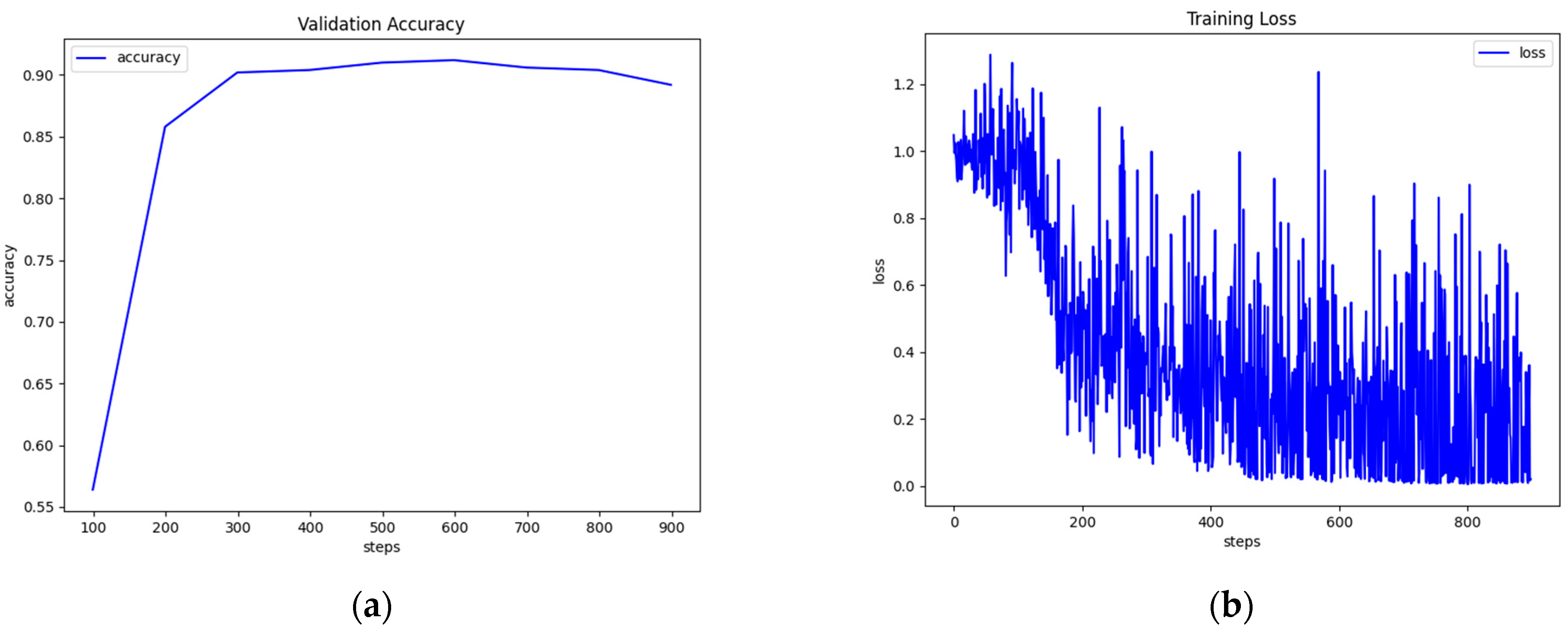
The best RoBERTa-base implementation (batch size 64, learning rate 4 × 10⁻⁵) was trained for 16,000 steps and exhibited 91.41% accuracy on the test set, 1.1% higher than BERT-base. RoBERTa-large raised the accuracy even more to 91.92% (Figure 1). RoBERTa -large was trained for 35,000 steps with a batch size of 16 and a learning rate of 2 × 10⁻⁵.

ALBERT’s performance was slightly worse than the other BERT models. The base version demonstrated 87.71% accuracy, and the large version demonstrated 89.96% accuracy. The base version was trained with a batch size of 64 and a learning rate of 4 × 10⁻⁵ for 12,000 steps, while the large version was trained with a batch size of 32 and a learning rate of 32 for 20,000 steps.

5.2. Results on SICK

The best DAM implementation demonstrated 81.10% accuracy on the development set and 83.37% on the test set. It was trained with a hidden layer size of 300, a batch size of 16, a learning rate of 0.01, a dropout rate of 0.2, and a weight decay of 10⁻⁵ for 34 epochs. Adding the intra-sentence attention did not improve performance, as our best implementation achieved 83.15% accuracy on the test set.

The best test set performance of the ESIM model was 80.81%, a slight drop in performance compared with DAM. We trained this implementation with a hidden state size of 300, a batch size of 16, the Adam optimizer with a learning rate of 0.0004, and a dropout rate of 0.5 for 15 epochs.

BERT-base’s best performance on the test set was 87.42%, a large improvement from the previous models. It was trained with a batch size of 32 and a learning rate of 3 × 10⁻⁵ for 640 steps, with the first 140 of those being warmup steps. Our best BERT-large implementation achieved 89.85% accuracy on the test set. We trained with a batch size of 16 and a learning rate of 2 × 10⁻⁵ for 1200 steps with 140 warmup steps.

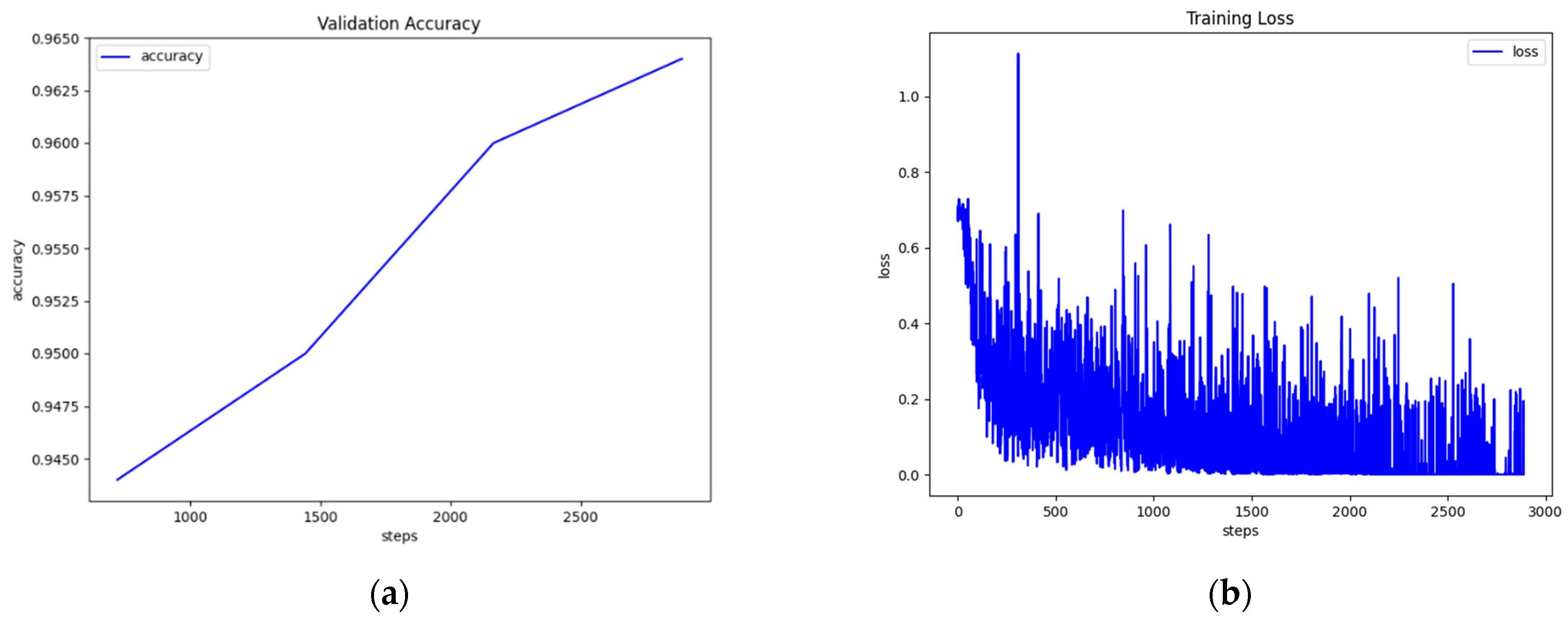
With RoBERTa-base, the best test set performance we achieved was 89.59%, a 2% jump from BERT-base. We trained the model with a batch size of 64 and a learning rate of 2 × 10⁻⁵ for 420 steps, with the first 70 steps as warmup steps. With RoBERTa-large, our best implementation demonstrated 91.50% accuracy on the test set, and it was trained with a batch size of 16, a learning rate of 10⁻⁵, and 140 warmup steps for a total of 900 steps (Figure 2).

Our best implementation of ALBERT-base achieved 89.06% accuracy on the test set. We trained the model with a batch size of 32, a learning rate of 2 × 10⁻⁵, and 140 warmup steps for a total of 720 steps. For ALBERT-large, our best implementation demonstrated 89.85% accuracy, which is the same as BERT-large, and was trained with a batch size of 16, a learning rate of 2 × 10⁻⁵, and 140 warmup steps for a total of 1200 steps.

5.3. Results on SciTail

The best DAM implementation on SciTail achieved an accuracy of 69.50% on the test set. We trained this model with a batch size of 64, and the AdaGrad optimizer with a learning rate of 0.025, a hidden layer size of 200, a dropout rate of 0.2, and a weight decay of 10⁻⁵ for 50 epochs. The intra-sentence attention model did not bring any further improvement, yielding an accuracy of 68.78% on the test set.

Our best ESIM implementations yielded an improvement of almost 5% compared with DAM, achieving 75.17% accuracy. This implementation was trained with a batch size of 32, a hidden state size of 200, and the AdaGrad optimizer with a learning rate of 0.01 and a dropout rate of 0.8 for 11 epochs.

With BERT-base, the best performance we observed was 93.65%, a huge jump from the previous models. We trained the model with a batch size of 64, a learning rate of 3 × 10⁻⁵, and 108 warmup steps for a total of 1200 steps. As for the large model, it performed slightly better (93.79%). The large model was trained with a batch size of 16, a learning rate of 3 × 10⁻⁵, and 577 warmup steps for a total of 5776 steps.

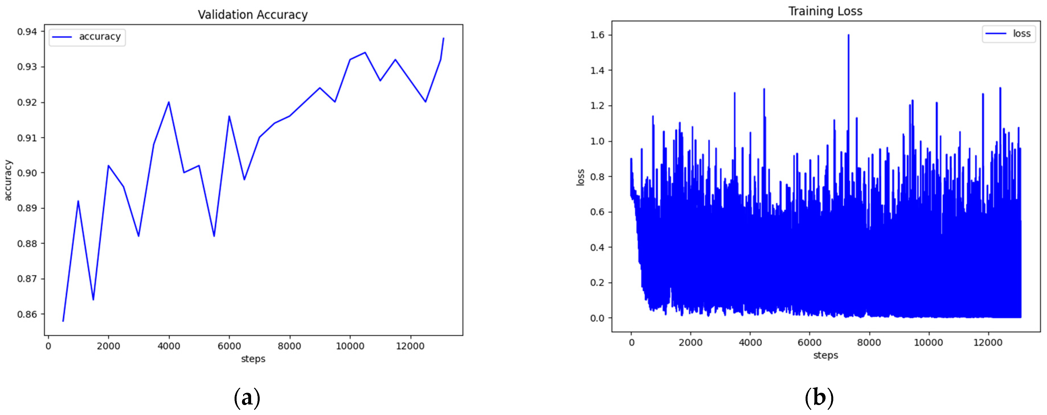
RoBERTa-base performed similarly to BERT-base on SciTail, reaching 93.51% accuracy on the test set. The model was trained with a batch size of 64, a learning rate of 4 × 10⁻⁵, and 72 warmup steps for a total of 722 steps. The large version, however, clearly outperformed RoBERTa-base, scoring 96.52 on the test set (Figure 3). This implementation was trained with a batch size of 16, a learning rate of 2 × 10⁻⁵, and 576 warmup steps for a total of 5776 steps.

With the ALBERT-base model, we obtained an accuracy of 94.21% on the test set, which is higher than the other base models. In this implementation, the model was trained with a batch size of 64, a learning rate of 3 × 10⁻⁵, and 144 warmup steps for 1444 steps. The ALBERT-large model scored an impressive 94.64% accuracy, which falls second only to RoBERTa-large. The model was trained with a batch size of 32, a learning rate of 3 × 10⁻⁵, and 288 warmup steps for 2888 steps.

5.4. Results on DNLI

Our best implementation of DAM on DNLI achieved 83.92% accuracy on the test set. The model was trained with a batch size of 32, a hidden layer size of 200, and the AdaGrad optimizer with a learning rate of 0.025 and a dropout rate of 0.2 for 22 epochs. Adding the intra-sentence attention step improved performance and raised the accuracy to 85.19%. The intra-attention model was trained with a bigger batch size (64) and a bigger hidden layer size (300), while the other hyperparameters stayed the same.

With the ESIM model, we scored an accuracy of 87.07% on the test set, a 2% increase from DAM. We trained ESIM with a batch size of 32, a hidden state size of 300, and the Adam optimizer with a learning rate of 10⁻⁵ and a dropout rate of 0.5 for 5 epochs.

Our best implementation of BERT-base on DNLI achieved 90.68% accuracy on the test set. In this implementation, BERT was trained with a batch size of 32, a learning rate of 10⁻⁵, and 969 warmup steps for a total of 9691 steps for 1 epoch. The large version of BERT performed 91.29% on the test set.

With the RoBERTa-base model, we achieved an accuracy of 91.42%, a slight increase from BERT-base. The model was trained with a batch size of 64, a learning rate of 4 × 10⁻⁵, and 484 warmup steps for a total of 4846 steps for 1 epoch. The large version of Roberta achieved 92.42% accuracy on the test set.

The ALBERT-base model’s best performance on DNLI scores an accuracy of 90.90%, falling in between BERT-base and RoBERTa-base. The model was trained with a batch size of 64, a learning rate of 10⁻⁵, and 484 warmup steps for 4846 steps for 1 epoch. The large version of ALBERT achieved 91.31% accuracy on the test set (Figure 4).

5.5. Results on MNLI

The best performance on MNLI with DAM was 72.52% on the matched development set. The model was trained for 175 epochs with a batch size of 64, a learning rate of 300, and the AdaGrad optimizer with a learning rate of 0.025 and a dropout of 0.2. The intra-attention model demonstrated no improvements, as it scored 69.96% on the development set.

With ESIM, we scored an accuracy of 76.8% after training for 5 epochs with a batch size of 32, a hidden state size of 300, and the Adam optimizer with a learning rate of 0.0004 and a dropout of 0.2. Raising the hidden state size to 600 further improved performance.

Our best implementation of BERT-base on MNLI achieved accuracies of 84.64% and 85.35% on the matched and mismatched development sets, respectively. This implementation was trained with a batch size of 32, a learning rate of 2 × 10⁻⁵, and 4910 warmup steps for 49,108 steps or 4 epochs. With the BERT-large model, we achieved accuracies of 86.56% and 86.17% on the matched/mismatched development sets, respectively. It was trained with a batch size of 16 and a learning rate of 10⁻⁵ for 3 epochs.

With the RoBERTa-base model, we scored accuracies of 87.94% and 87.72% on the matched/mismatched development sets, respectively. The model was trained with a batch size of 64, a learning rate of 2 × 10⁻⁵, and 1842 warmup steps for 3 epochs. RoBERTa-large’s best performance was a score of 90.52%/90.25% accuracy on the matched/mismatched development sets, respectively, a large increase from the previous scores (Figure 5). It was trained with a batch size of 16, a learning rate of 10⁻⁵, and 1842 warmup steps for 3 epochs.

The best performance of ALBERT-base was 85.80% accuracy on the matched development set; it was trained with a batch size of 64 and a learning rate of 4 × 10⁻⁵ for 1 epoch with a warmup ratio of 0.1. The large version achieved 88.60% accuracy when trained with a batch size of 32 and a learning rate of 2 × 10⁻⁵ for 2 epochs with a warmup ratio of 0.1.

5.6. Results on QNLI

With DAM, the best performance on QNLI was 75.01% accuracy on the development set. The model was trained with a batch size of 32, a hidden layer size of 200, and the AdaGrad optimizer with a learning rate of 0.025 and a dropout rate of 0.2 for 49 epochs. The same accuracy was obtained with the intra-attention model.

The ESIM model performed higher (81.16%) on the development set of QNLI. It was trained with a batch size of 64, a hidden state size of 300, and the Adam optimizer with a learning rate of 0.0004 and a dropout rate of 0.5 for 8 epochs.

The BERT-base model raised the accuracy even more, scoring 89.36% on the development set in the 4th epoch of training, although validation loss increased after the 2nd epoch. The hyperparameters used were a batch size of 64, a learning rate of 3 × 10⁻⁵, and a warmup ratio of 0.15. The large version performed slightly higher (90.54%) in terms of accuracy, and it was trained with a batch size of 16 and a learning rate of 10⁻⁵ for 4 epochs with a warmup ratio of 0.1. We observed the same pattern on the validation loss with BERT-base.

RoBERTa-base achieved an accuracy of 90.77% when trained for 4 epochs with a batch size of 32, a learning rate of 2 × 10⁻⁵ and a warmup ratio of 0.1. The large version scored an even higher accuracy (93.21%). It was trained for 4 epochs with a batch size of 16, a learning rate of 10⁻⁵, and a warmup ratio of 0.2.

ALBERT-base achieved 93.80% accuracy on QNLI, 0.6% higher than the large version of RoBERTa. It was trained with a batch size of 32 and a learning rate of 2 × 10⁻⁵ for 1 epoch or 3.274 steps, with the first 327 being warmup steps. The large version achieved the same accuracy of 93.80% (Figure 6). This model was trained with a batch size of 16, a learning rate of 10⁻⁵, and 1.309 warmup steps for 13.094 steps.

5.7. Results on RTE

Τhe best performance of DAM on the RTE development set was 68.20%. This accuracy was achieved by training the model with a batch size of 64, a hidden layer size of 200, and the Adam optimizer with a learning rate of 0.0001 and a dropout of 0.5. The model achieved the highest accuracy on the 25th epoch, and improvement stopped after that. With the inclusion of intra-attention, we observed similar patterns, with the highest accuracy score being 63.48%.

The ESIM model performed even worse than DAM, scoring an accuracy of 61.49%. This was the best score and was achieved by training with a batch size of 64, hidden state size of 200, and the Adam optimizer with a learning rate of 0.0001 and a dropout of 0.5 for 16 epochs. The highest accuracy was achieved on the 11th epoch.

With BERT-base, as with all transformers, we first trained the model on MNLI and then on RTE training data. This improved performance on the evaluation data of RTE. BERT-base achieved an accuracy of 83.75% on RTE. We trained the model with a batch size of 64, a learning rate of 2 × 10⁻⁵, and 24 warmup steps for 240 steps. BERT-large’s highest accuracy on RTE was 84.48%. We trained BERT-large with a batch size of 16, a learning rate of 2 × 10⁻⁵, and 30 warmup steps for 300 steps in total.

The best performance with RoBERTa-base was 87.36%, a large improvement compared to BERT-base. We trained RoBERTa-base with a batch size of 64 and a learning rate of 2 × 10⁻⁵ for 280 steps, with the first 28 being warmup steps. The large version’s best performance was 90.97% (Figure 7), a 6.5% increase from BERT-large. RoBERTa-large was trained with a batch size of 16 and a learning rate of 10⁻⁵ for 200 steps with 20 warmup steps.

ALBERT base’s best performance on RTE was 84.48%, 0.73% higher than BERT-base and equal to BERT-large. It was trained with a batch size of 64, a learning rate of 10⁻⁵, and 20 warmup steps for 200 steps. The large version of ALBERT performed equally well as the base version scoring 84.47% accuracy on the development set. It was trained with a batch size of 16, a learning rate of 2 × 10⁻⁵, and 60 warmup steps for 600 steps. We believe the reason the accuracy is not higher is that the model was not finetuned well enough on MNLI.

5.8. Results on WNLI

The best performance we obtained from DAM on WNLI was 76.00%. The model was trained with a batch size of 200, a hidden layer size of 200, and the AdaGrad optimizer with a learning rate of 0.05 for 100 epochs. Similar results were obtained with the intra-attention model.

ESIM’s best performance on WNLI was 67.55%, a huge drop compared to DAM. This model was trained with a batch size of 64, a hidden state size of 200, and the Adam optimizer with a learning rate of 0.0001 and a dropout of 0.5 for 40 epochs. In the first 20 epochs, the validation accuracy was stuck at 67.55% and then dropped dramatically with every epoch. Likewise, the validation loss increased after the 20th epoch.

All BERT models performed random chance on WNLI. The reason was that WNLI contains adversarial examples in the validation set, which punishes models for learning the training data. There were some published workarounds for WNLI, but we chose to ignore the results for this dataset.

5.9. Discussion

In

Table 2. Accuracies (%) of the best implementations on test data. We use validation data (*) when test data are not publicly available. For MNLI, we present the results for the matched dataset. The best results are in bold.

Model	Params	SNLI	SICK	SciTail	DNLI	MNLI *	RTE *	QNLI *	WNLI *
DAM	382 K	85.13	83.37	69.50	83.92	72.52	68.20	75.01	76.00
ESIM	4.3 M	87.07	80.81	75.17	87.07	77.59	61.49	81.16	67.55
BERT-Base	110 M	90.34	85.71	93.65	90.68	84.64	83.75	89.36	60.56
BERT-Large	340 M	90.63	89.85	93.79	91.09	86.56	84.48	90.54	60.56
RoBERTa-Base	125 M	91.41	89.59	93.51	91.42	87.94	87.36	90.77	56.34
RoBERTa-Large	355 M	91.92	91.50	96.52	90.87	90.52	90.97	93.21	56.34
ALBERT-Base	11 M	87.71	89.06	94.21	90.90	85.80	84.48	93.80	59.15
ALBERT-Large	17 M	89.96	89.85	94.64	91.50	88.60	84.47	93.80	61.97

, the best accuracies of each model on each of the eight datasets are presented. The most obvious observation is that the pre-trained transformers very clearly outperform the older models. The differences in accuracies between them are 0.64–20%. Out of the three BERT models, RoBERTa comes out to be the best performing one, given that its large version has the highest accuracy on almost all tasks. This is a trend across all BERT models; larger models perform better than their base versions. ALBERT seems to do exceptionally well, given its size. It generally performs comparative results with respect to the other two, and in one dataset (QNLI), it outperforms all others. Better performances can be achieved with ALBERT’s xlarge and xxlarge versions, but we are more interested in looking at the inference capabilities of the smaller versions.

One dataset that proved to be more of a challenge to the BERT models is RTE. It took an MNLI fine-tuning approach to achieve results above 80%. Even then, it is the hardest dataset we tried, and only RoBERTa-large managed to break the line of 90% accuracy. This was also true with the MNLI task. The easiest task to solve, on the other hand, seems to be SciTail. All models performed well above 90%, with RoBERTa-large scoring 96.52% on the test set. One explanation is that Wikipedia, where all BERT models were trained, contains the answers to the science questions in SciTail.

In

Table 3. Comparison of the state-of-the-art models on well-known datasets with our best model (RoBERTa-Large) in terms of accuracy (%). The best results are in bold, the second best underlined.

Model	MNLI	RTE	QNLI	SNLI	SciTail
BERT-Large [10]	86.7	70.4	92.3
ALBERT-Large [25]	90.8	89.2	95.3
SMART-BERT [38]	85.6	71.2	91.6	91.1	93.2
HyPe-RoBERTa [39]	90.32		94.19
PowerQuant-BERT [40]	80.54	61.82	91.47
RoBERTa-Large [24,41]	90.2	86.6	94.7	91.2	96.0
Our-RoBERTa-Large	90.52	90.97	93.21	91.92	96.52

, a comparison of the best of our models (RoBERTa-Large) with state-of-the-art approaches is attempted. In the table, we have included models that deal with the same datasets. It is evidence that our model does better than the others on three datasets (RTE, SNLI, SciTail), especially on the RTE, which is one of the toughest, and is second on one (MNLI).

6. Testing Generalization

Although accuracy on the test set is a measure of the effectiveness of a model and shows the generalization capability of the model on unknown data from the same dataset as the training set, it does not assure the generalization capability of the model on data from other similar datasets. To evaluate such a generalization capability, we used two methods, as follows.

6.1. Breaking NLI Test

We attempted to “break” our models by testing them on the breaking NLI dataset. This dataset was created for testing trained NLI models regarding their generalization. It consists of examples that differ by, at most, one word from sentences in the training set, but the performance of well-known trained models is substantially reduced on that set [42]. In our case, for training data, we used SNLI and MNLI. The results of the Breaking NLI set are shown in

Table 4. Accuracies (%) of the models on Breaking NLI test set trained on SNLI and MNLI. The best results are in bold.

Model	SNLI	MNLI
DAM	31.60	30.11
ESIM	55.68	64.05
BERT-Base	87.28	90.89
BERT-Large	92.68	94.54
RoBERTa-Base	93.21	94.50
RoBERTa-Large	96.39	96.47
ALBERT-Base	93.94	92.89
ALBERT-Large	96.92	95.69

. We see that DAM and ESIM cannot handle the test set sufficiently. In the case of DAM, the accuracy is at the level of random chance. The BERT models, on the other hand, perform exceptionally well, almost all above 90%, whether they are trained on SNLI or MNLI. The best performance comes from RoBERTa-large, trained on MNLI, and ALBERT-large, trained on SNLI.

6.2. Talman and Chatzikyriakidis’ Test

The second method is presented in [30]. According to that, a model was developed based on a dataset and was tested on a different dataset. Therefore, to evaluate the generalization capabilities of the above models in conjunction with the used datasets, we conducted several experiments. First, we configured and evaluated the eight deep learning models based on each of seven (out of eight) datasets, i.e., using a training and a test set from the same dataset, which are the baseline models. Then, we configured and evaluated the eight deep learning models based on pairs of the seven datasets; that is, the training set was from one dataset, and the test set wasfrom the other dataset. In this way, we tested how well a trained model based on a dataset generalizes when it is used on a different dataset.

The results in terms of the largest and smallest drops in accuracy in relation to baseline models are presented in

Table 5. The largest and smallest drops in accuracy (%) of models trained on data of three labels belonging to a different dataset from that of test data, with reference to the baseline models (trained on data from the same dataset as the test set). Data with (*) are validation data.

Training Data	Test Data	Largest Drop in Acc.		Smallest Drop in Acc.
		Value	Model	Value	Model
MNLI	SNLI	11.43	DAM	2.49	RoBERTa-Large
MNLI	SICK	31.90	ALBERT-Large	19.05	ALBERT-Base
MNLI	DNLI	22.01	RoBERTa-Large	14.28	DAM
SNLI	MNLI *	25.34	ESIM	8.57	RoBERTa-Large
SNLI	SICK	33.70	DAM	25..07	ALBERT-Base
SNLI	DNLI	42.93	DAM	24.95	ROBERTA-Base
SICK	MNLI *	48.24	ALBERT-Large	36.75	ESIM
SICK	SNLI	48.79	ALBERT-Large	37.57	BERT- Base
SICK	DNLI	50.42	ALBERT-Base	37.24	DAM
DNLI	MNLI *	55.57	ALBERT-Base	46.42	DAM
DNLI	SNLI	54.17	ALBERT-Large	35.42	BERT-Base
DNLI	SICK	59.43	BERT-Large	48.18	ESIM

(for the datasets that use three labels) and in

Table 6. The largest and smallest drops in accuracy (%) of models trained on data of two labels belonging to a different dataset from that of test data, with reference to the baseline models (trained on data from the same dataset as the test set). Data with (*) are validation data.

Training Data	Test Data	Largest Drop in Acc.		Smallest Drop in Acc.
		Value	Model	Value	Model
QNLI	SCITAIL *	25.99	ALBERT-Base	16.49	DAM
QNLI	RTE	44.15	ALBERT-Base	30.60	DAM
SCITAIL	QNLI	41.96	RoBERTa-Large	18.00	DAM
SCITAIL	RTE	30.97	BERT-Base	18.84	ESIM
RTE	QNLI	27.93	RoBERTa-Large	10.04	ESIM
RTE	SCITAIL *	24.04	DAM	−14.19	BERT-Large

(for the datasets that use two labels). The full results for both cases are presented in Appendix A.

Testing generalization from MNLI to SNLI (Table 5), we find that the largest drop from baseline is that of DAM (11.43%) and the smallest is that of RoBERTa-large (2.49). The transformers generalize well to SNLI, having the largest drop in accuracy of 6.31% from baselines. The opposite, however, brings some interesting results. Generalizing from SNLI to MNLI, we observe a much larger drop in accuracies from the baselines. The best-performing model is still RoBERTa-large, with a drop of 8.57% in accuracy, while the drop in performance of the rest of the transformers ranges from 12% to 18%. The non-transformer models perform even worse, with a drop of around 25%. The conclusion for this dataset pair is that MNLI is harder than SNLI and creates models with better generalization.

Generalizing from MNLI to SICK, we find that performance drops at a high rate regardless of the model. In this case, the non-transformers are not the worst-performing models, as they suffered a drop of 23% from the baselines. The worst performance came from the large models, with BERT-large having a drop of 31.32%, RoBERTa-large a 30.9% drop in accuracy, and ALBERT-large having a 31.9% drop in accuracy. The base models had the best generalization score, with ALBERT-base having the best of those (60.84%) with a drop of 19.05%. Generalizing from SICK to MNLI, however, doubles the drop in performance difference from baseline. All the models fail on MNLI when trained on the SICK training set. The best-performing model is BERT-base, with an accuracy of 48.29% and a drop of 39.34%. We see a much larger difference between these two datasets, as MNLI is a newer and more difficult set. Therefore, models trained on MNLI generalize better than those trained on SICK.

Next, we compared MNLI and DNLI as far as their generalization capability is concerned. The best generalization performance from MNLI to DNLI came from RoBERTa-base, demonstrated an accuracy of 69.2%. The largest drop from baseline came from RoBERTa-large. Both DAM and ESIM dropped their accuracy by 14% from their baseline, with ESIM achieving 62.12% accuracy, which was a higher score than some of the transformers. The opposite generalization failed across all the models. Allmodels performed just above random chance, with the best being RoBERTa-large with a 41.38% accuracy, representing a 50% drop from the baseline. This decrease notably points out the simplicity, and hence, the weak generalization, of DNLI.

Testing generalization from SNLI to SICK brought results that are comparable to those of MNLI to SICK. The best-performing model was ALBERT-base, with an accuracy of 61.42%, which means a drop of 25.07% from baseline. Non-transformers stayed at around 50%, with a drop of 33%. The opposite generalization testing gave far worse results, as expected. The models cannot learn the task of SNLI, and performance across all models was below 50%, except for BERT-base, which scored a 50.06% accuracy, resulting in a drop of 37.57%. The non-transformer models performed just above random chance, both at around 36% accuracy.

Comparing SNLI and DNLI, we found that the best-performing model was both versions of RoBERTa, with the best being RoBERTa-base with a 62.00% accuracy and a drop of 24.95%. The rest of the transformers performed just above 50%, and the non-transformers were even lower than that. The best model to generalize from DNLI to SNLI was BERT-base, with a score of 54.53% and a drop of 35.42%. The large transformers performed worse than the base versions in this experiment, scoring accuracies comparable to the non-transformers.

Finally, we tested generalization between the two lowest-scoring models, SICK and DNLI. Only one model passed the 50% mark, and that was BERT-base; the rest of the models exhibited lower scores. Generalizing from DNLI to SICK resulted in the lowest scores out of all the experiments, with the best being the 42.38% accuracy of RoBERTa-base.

As far as two-label classification is concerned (Table 6), testing generalization from QNLI to SciTail, we observed the smallest drop from RoBERTa-large and the largest from ALBERT-base. Both ALBERT versions had trouble solving SciTail, as both scored less than 70% in accuracy. The best accuracy score was obtained by RoBERTa-large at 77.28%. Generalizing from Scitail to QNLI, we observe huge drops in the accuracies of all models. All transformers scored just above random chance with a drop of around 40%, while the non-transformers also scored random chance level accuracies with a drop of about 20%.

Generalization from QNLI to RTE seems to be difficult for all models. The best score was from RoBERTa-large (62.45%), with a drop of 31.78%. Once again, the large versions performed better than the base versions, but still, the performances are around random chance levels. The older models performed even worse, at around 40% accuracy. The opposite generalization did not result in better results, as all models performed at random chance levels.

Testing generalization from Scitail to RTE, we found a decent performance from RoBERTa-large (71.11%), with a drop of 23.71%. The rest of the transformers performed only just above 60%. However, the opposite generalization brought the most interesting results of all the comparisons. The transformers, when trained on RTE and tested on SciTail, achieved scores above 80%. The best one was RoBERTa-large’s performance (84.76%) with a drop of −4.98%, which is an increase in accuracy compared to baseline. The largest increase (negative drop) was that of BERT-large, which was the only case where we observed negative values of drop. Table 5 and Table 6 show the results of the generalization test on the three-way and two-way classification tasks. In Table 5, we see that the generalization from MNLI to SNLI has the smallest drop from baseline. This is due to the sets’ similarity in size and collection method. However, the opposite is not true because MNLI is a harder dataset to solve than SNLI. In general, MNLI has the best performance out of the four datasets, but still, the losses in the generalization ability are far from negligible. The worst performances are observed when generalizing from DNLI and SICK. When comparing the models, we see similar behaviors between the pre-trained transformers.

6.3. Implementation Details

The generalization experiments for the non-transformer models were carried out using the GluonNLP toolkit. We trained the models, saved them and then tested them against the test sets from all the other datasets. For the transformer models, we used the JiantNLP toolkit. Each time we configured it to train on a single training and development set while including all the test sets. For all our experiments, we chose the hyperparameters based on the models’ performance in our previous experiments. The complete list of hyperparameters is shown in Appendix B.

7. Conclusions

Our findings show that pre-trained transformer models are very good at solving different NLI tasks. We observed high accuracies on all datasets we tried, even on Breaking NLI, where the older models failed. This shows that these models have a better understanding of language and better world knowledge. We also observed that the larger versions of the transformers performed better, but we also saw very good results from ALBERT, which has 18 times fewer parameters. However, all models, including transformers, fail to generalize across different NLI datasets. We believe this is attributed to the quality and collection method of each NLI dataset. This becomes evident when generalizing from MNLI to SNLI, which provides decent results due to their similarity. Talman et al. believe that each dataset evaluates a different type of inference ability, making it hard for models to generalize [30]. We agree with this conclusion since we experimented with the two most powerful transformers (RoBERTa and ALBERT) with no further improvement on the generalization test.