Decoupled Monte Carlo Tree Search for Cooperative Multi-Agent Planning

Abstract

The number of agents exponentially increases the complexity of a cooperative multi-agent planning problem. Decoupled planning is one of the viable approaches to reduce this complexity. By integrating decoupled planning with Monte Carlo Tree Search, we present a new scalable planning approach. The search tree maintains the updates of the individual actions of each agent separately. However, this separation brings coordination and action synchronization problems. When the agent does not know the action of the other agent, it uses the returned reward to deduce the desirability of its action. When a deterministic action selection policy is used in the Monte Carlo Tree Search algorithm, the actions of agents are synchronized. Of all possible action combinations, only some of them are evaluated. We show the effect of action synchronization on different problems and propose stochastic action selection policies. We also propose a combined method as a pruning step in centralized planning to address the coordination problem in decoupled planning. We create a centralized search tree with a subset of joint actions selected by the evaluation of decoupled planning. We empirically show that decoupled planning has a similar performance compared to a central planning algorithm when stochastic action selection is used in repeated matrix games and multi-agent planning problems. We also show that the combined method improves the performance of the decoupled method in different problems. We compare the proposed method to a decoupled method in regard to a warehouse commissioning problem. Our method achieved more than 10% improvement in performance.

1. Introduction

Cooperative multi-agent planning involves coordinating the actions of multiple agents with a common objective and a willingness to work together towards a shared goal. While this type of planning can be less complex than non-cooperative planning, where agents may have conflicting goals or limited communication, it still requires careful coordination and consideration of the actions and capabilities of each agent. The number of possible combinations of actions that each agent can take can still grow exponentially with the number of agents. In addition, the environment in which the agents are operating may be dynamic and subject to change, requiring the plan to be flexible and adaptable.

All these challenges of cooperative multi-agent planning render the problem intractable for most interesting problems, such as warehouse commissioning. In a warehouse setting, there may be multiple agents with different capabilities and resources, working in a dynamic environment with constantly changing demands and constraints. Coordinating the actions of these agents to efficiently complete tasks can be a complex and computationally intensive task. Traditional optimization methods may not scale well to these types of problems, and even with advanced algorithms, finding an optimal solution may be impractical, due to the time and computational resources required. As a result, finding effective approaches to cooperative multi-agent planning in warehouse commissioning, and other similar problems, is an active area of research.

In this paper, we aimed to improve the scalability of cooperative multi-agent planning using online planning. Online planning involves making decisions and taking actions in real-time, as new information becomes available, rather than solving the problem in advance. This can be particularly useful in dynamic environments, where the problem may change rapidly, or in problems with large state spaces, where the computational cost of solving the problem in advance may be prohibitive. Monte Carlo Tree Search (MCTS) is one of the well-known online planning algorithms for complex problems. MCTS does not require a full model of the process. Instead, a black-box simulator, the definition of state, and action space is enough for MCTS.

The MCTS algorithm plans over the joint actions of agents. The joint action set is constructed as the Cartesian product of the actions of agents. The planning algorithm calculates a single joint action for the given state. Agents execute the assigned actions independently. Although this approach works well, it creates an exponential increase in the state and action space of the problem. To reduce this exponential increase, we propose using decoupled planning. When the MCTS algorithm is used as a planning algorithm, we call it decoupled MCTS. In decoupled MCTS, every agent plans independently, but the same joint reward of the simulation is used. This approach results in a linear increase in state and action space but suffers from local optimum results [1]. In our experiments, we showed that this approach achieved reasonable performance, compared to the baseline methods such as MCTS over joint actions.

When decoupled MCTS uses deterministic action selection policy in cooperative problems, the action synchronization problem occurs. This is due to the propagation of the same reward value for each agent. Although decoupled MCTS is widely used in regard to general game-playing problems [2,3,4,5,6,7], they do not report such a problem, even for cooperative games. In cooperative problems, each decoupled agent chooses an individual action, then, these actions are combined and executed for the problem and, finally, a reward is taken. This reward updates all agents’ actions, but these updated actions constitute only one of the combinations of all agents’ actions. This combination has the same statistics. If a deterministic action selection policy is used, the actions of that combination are chosen together since they have the same statistics. To remedy this problem, we propose to use stochastic action selection policies where the action selection for each agent is a result of a stochastic process. We evaluated different stochastic action selection policies on different problems and showed that $ϵ$-greedy had the best performance for most of the problems.

We also identified a miscoordination problem in decoupled MCTS planning. When the agents do not coordinate their selection of actions, their performance decreases depending on the problem. This is common, especially for problems having penalties for miscoordination. We propose a combination method on top of decoupled MCTS. After the decoupled MCTS, a centralized MCTS search tree is constructed using the individual action evaluations of decoupled MCTS. Since the construction of all possible joint actions is intractable, we generate a subset of joint actions. The joint actions are chosen based on the statistics of individual actions constituting the joint action. We showed that this method improves the performance of decoupled MCTS when the search is not shallow.

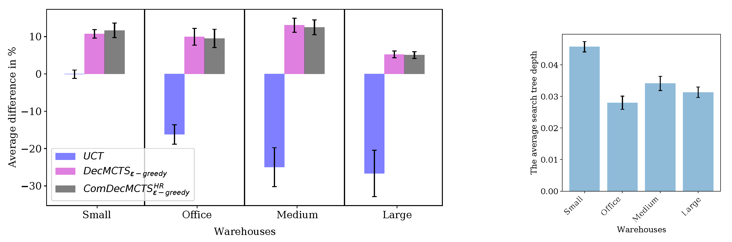
We compared our proposed method with the state-of-the-art decoupled planning method [8] from the literature. We showed that our method outperformed it with a performance improvement of more than 10% in warehouse commissioning problems. We also report that our method is easy to generalize to all sets of multi-agent planning problems because it does not require a greedy algorithm to represent the other agents’ behaviors.

The contributions of the paper can be summarized as follows:

• We present a unique problem in decoupled MCTS planning that occurs when deterministic action selection policies are used and propose to use stochastic action selection policies to solve it.
• We present the coordination problem in decoupled MCTS and propose to combine the evaluation of individual actions to plan over joint actions.
• We analyze different cooperative problems and show the limitations of decoupled MCTS when a combination strategy is used.

In Section 2 we provide a short survey of the literature by summarizing the work done on the different aspects of multi-agent planning. We present the problem description in Section 3. In Section 4, we provide a brief background on Monte Carlo Tree Search. We present the proposed decoupled planning approach in Section 5. In Section 6, we show the results of the experiments in different settings. Finally, we provide the conclusions in Section 7.

2. Related Work

There are two main issues in multi-agent planning; coordination and the curse of dimensionality. The coordination problem arises when agents execute actions without the knowledge of other agents. In literature, there are three main approaches to handle the coordination problem; coordination-free, coordination-based, and explicit coordination [9]. Coordination-free methods just ignore the problem and assume that the optimal joint action is unique. Coordination-based approaches use the coordination graph to decompose the value function over agents. The value function calculates an expected cumulative reward of the joint state. Explicit coordination mechanisms generally use a social convention or communication to determine a global ordering of agents and their actions [10]. Our method used a coordination-free approach, where we assumed that the optimal joint action was unique.

The curse of dimensionality problem results from the Cartesian product of the action sets and state sets of agents. Goldman and Zilberstein categorized the cooperative decentralized planning problems in terms of model specializations, and communications [11]. They showed that Decentralized Partially Observable Markov Decision Processes (Dec-POMDP) with independent observation and transition functions have NP-complete complexity and are a lot simpler than the original Dec-POMDP model (NExp-Complete [12]). Even further specializations, such as having a single goal state and uniform cost, reduce the complexity to P-complete [13]. They also showed that having direct communication between agents did not change the complexity class of decision processes. The decision–theoretic model of the problem targeted in this work was the Multi-agent Markov Decision Process (MMDP). The complexity of the MMDP is the same as MDP, except for the exponential increase in the action and state space. MMDP problems have the curse of dimensionality due to the number of agents. Therefore, we attacked the curse of dimensionality problem by representing every agent as an independent planner. However, representing every agent as an independent planner required a special mechanism to solve the coordination problem [1,14].

Lauer and Riedmiller presented a decentralized reinforcement learning algorithm for deterministic multi-agent domains [15] where the coordination problem was solved using a special mechanism. The algorithm made use of the deterministic nature of the problem, such that agents could infer other agents’ actions using the next state and reward that was observable. However, every agent iteratively improved its policy and achieved coordination via updating its policy only in the case of improvement. That eliminated the accumulation of two or more actions having the same expected sum of rewards, and, therefore, policies chose one of the equilibrium points and solved the coordination problem. Peshkin et al. proposed another method for a decentralized policy search algorithm for cooperative multi-agent problems [16]. They assumed that agents had local policies that mapped the local states of the agents to the actions. They showed that a decentralized policy search could learn local optimal policies using the gradient descent algorithm.

Gronauer et al. presented the challenges of multi-agent problems in the deep reinforcement learning domain [17]. They listed non-stationarity and coordination under the distributed training of cooperative problems. However, these challenges are also valid for online planning methods, because they use the same mathematical formalism [18]. The value-based reinforcement learning methods address these challenges by summarizing the effect of other agents [19,20]. Another line of research uses a coordination graph [21] to decouple the agents and build a new formalism to describe the influence of agents to each other [22]. In addition to the multi-agent research, there are single-agent approaches that reduced the action complexity by converting the problem into a multi-agent one and achieved comparable performances [23,24].

There are methods based on Monte Carlo Tree Search (MCTS) that model agents independently in distributed planning. Best et al. presented a method for active robot perception, where each robot shares its search tree and the agent calculates a distribution over action sequences [25]. Their formalism was limited, compared to ours, as the policies were represented as action sequences. Amini et al. presented a similar method for partially observable problems where the agents were modeled over joint action spaces [26]. This made their method intractable, due to the exponential action space. Czechowski et al. presented a decoupled MCTS method that uses alternate maximization over independent search trees [27]. Although their method was guaranteed to converge, the agent policies were modeled with a neural network that was computationally expensive to train.

Another line of work that uses decoupled planning comes from the general game-playing literature. Finnsson and et al. used decoupled UCT for general game playing and won the General Game Playing tournament twice [2]. In game-playing, the planner models the opponent as another independent learner. Since agents get different rewards based on the state of the game, using deterministic action selection policies does not face the action synchronization problem. Decoupled planning was also applied to simultaneous move games where the agents take action without seeing the other agents’ actions [4,6,7,28]. They showed that different action selection policies had different performances for different games. Shafiei and et al. showed that UCB1-based decoupled planning was not guaranteed to converge to Nash-equilibrium [3] when used for simultaneous move games. Since in our decoupled planning setting, agents took actions without seeing the other agents’ actions, our problem formulation was similar to simultaneous move games. This was also the main motivation of this paper to use decoupled planning for cooperative multi-agent problems. There are different applications of decoupled planning in different domains [25,26,29], but they do not report on the action synchronization problem.

3. Problem Description

Cooperative multi-agent planning problems have different formulations. In this paper, we aimed to solve problems modeled as Multi-agent Markov Decision Process (MMDP). MMDPs are widely studied powerful representations for a class of problems where the next state only depends on the current state and the action of the agents.

Multi-Agent Markov Decision Process

Stochastic sequential decision-making problems can be modeled as Markov Decision Processes (MDPs). The MDP model defines the state space of the problem, available actions at every state, the probability of resulting states after executing an action, and the reward, given the current state, the next state, and the executed action. The solution to an MDP problem is called policy. Policies define state-action mapping. The optimal policy has the maximum expected cumulative reward given the MDP model. Calculating a policy for problems having huge state and action spaces is infeasible. The online planning approach solves this problem by only calculating the next most successful action. It evaluates only a subset of state and action spaces up to a limited time step by sampling actions from the given state.

To be able to plan for multiple agents, the action set is redefined as the Cartesian product of every agent’s action set, and this is called the joint action set. The main problem with multi-agent planning is the exponential increase in the space of actions and states, due to the number of agents. The MDP problem with many agents is called Multi-agent MDP (MMDP). In MMDP formalization, it is assumed that all agents can see the full state, and planning is done by a centralized entity.

The formal definition of MMDP is 5-tuple $\langle D,S,A,T,R\rangle$ where:

• D is the set of agents,
• S is the finite set of states,
• A is the finite set of joint actions ($A_1\times A_2\times ·\times A_n$),
• T is the transition function which assigns probabilities for transitioning from one state to another given a joint action, and
• R is the immediate reward function.

The online planning approach presented in this paper can be used for MMDP problems. However, it does not need the full MMDP definition. It is enough to have the generative model of the problem with state and action definitions. This makes a huge difference, because, for most of real-world problems, it is easy to define a black-box generative model without knowing or calculating the transition probabilities. For all of the problems we used in the experiments, we had a generative model, including for the warehouse commissioning problem.

4. Background

4.1. Monte Carlo Tree Search

The Monte Carlo Tree Search (MCTS) algorithm [30,31] builds a search tree using Monte Carlo simulations starting from the current state. At first, there is only the root node denoting the current state. Every simulation adds a new node to the tree. Nodes keep the statistics of the actions that are available at that state. As the search tree grows, the simulation selects actions using the statics of the node. When the simulation reaches one of the leaf nodes, the action selection is handled by the rollout algorithm without expanding the search tree. Finally, at the end of each simulation run, a new node is added to the leaf node and all the visited nodes during the simulation are updated by the cumulative reward, as seen in Figure 1.

MCTS is a general method used in general game playing and MDP problems. One of the important factors that affects the performance of the method is the action selection policy. The action selection policy determines the selection of an action given the statistics about the actions of a state. The action selection problem is handled as a multi-armed bandit and shown to have very good performance for problems having large state spaces [2,32,33].

4.2. Action Selection Policies for Monte Carlo Tree Search

At the nodes of the search tree, an action is chosen from the available ones at that state. However, based on the reward taken from each action, an algorithm decides to either exploit the best action or explore one of the other actions. This algorithm is called the action selection policy. There are two groups of action selection policies: deterministic and stochastic. The deterministic policies produce the same selection of the action given the same statistics. However, the stochastic policies choose the actions through some random events, such as sampling the actions according to the calculated probabilities. In general-game playing literature, if the optimal policy is a mixed strategy, or there are adversarial players, that policy can be approximated only by a stochastic policy [34,35]. However, for MDP problems, it is shown that deterministic policies have the best performance [32] in terms of regret.

4.2.1. Deterministic Policies

Deterministic action selection policies choose the same action given the same statistics. The nodes keep the number of visits, the number of selections for each action, and the reward taken as a result of the action.

One of the well-known deterministic action selection policies is Upper Confidence Bounds (UCB1) [32,36]. It is shown that the action selection at each node can be handled as an independent multi-armed bandit problem and has a good performance for large MDP problems [32]. When the algorithm reaches the action selection part, it gives priority to the actions of the state which were not previously explored. This is so as to let each action have statistics before comparing them using UCB1. When all the actions of the state are taken at least once, the algorithm calculates the UCB1 value of each action according to the Equation (1):

$$\begin{array}{c}\hfill Q(n,a)=\frac{{\sum }_i^{n_a}{R}_i}{n_a}+C\sqrt{\frac{lnN}{n_a}}\end{array}$$

(1)

The function Q represents the evaluation of expected cumulative rewards for each search node and action. The $R_i$ denotes the cumulative reward taken in the simulation i by following the action a from node n. C is a constant which is used to scale the exploration term. N stands for the number of visits to the node n. $n_a$ stands for the number of action a taken in node n. The action with the highest UCB1 value is selected.

4.2.2. Stochastic Policies

The stochastic action selection policies use the statistics of each action to calculate a random event and choose the action as a result of this. Most commonly, a stochastic policy may calculate a probability distribution over actions and sample an action according to this. The stochastic action selection policies are best suited for adversarial and stochastic bandit problems [37]. For such problems, the reward distributions may change at every simulation in unknown ways. In this study, we investigated two stochastic action selection policies:

• $ϵ$-greedy
• EXP3

$ϵ$-greedy action selection policy chooses actions uniformly with the probability of $ϵ$. The action having the maximum average cumulative reward is selected with the probability of $1-ϵ$. Therefore, there is direct control on the exploration and exploitation behaviors.

EXP3 (Exploration–Exploitation with Exponential weights) [34] is one of the well known stochastic action selection policies. The policy maintains a weight value for each action and calculates a probability from it. The probability of an action is calculated by the Equation (2):

$$\begin{array}{c}\hfill p_i=(1-\gamma )\frac{w_i}{{\sum }_j^K{w}_j}+\frac{\gamma }{K}\end{array}$$

(2)

$p_i$ represents the probability of action i. $w_i$ represents the weight of the action i. All weights are initialized to 1 at the beginning. K denotes the number of actions. $\gamma$ is a parameter that determines how much uniform action selection is favored. As $\gamma$ gets closer to 1, the action probabilities get closer to uniform probabilities ($1/K$). After an action is selected and executed, a reward $r_i$ is taken. The weights are updated according to the Equation (4):

$$\begin{array}{cc}\hfill \widehat{r_i}& =\frac{r_i}{p_i}\hfill \end{array}$$

(3)

$$\begin{array}{cc}\hfill w_i& =w_i{e}^{\gamma \widehat{r_i}/K}\hfill \end{array}$$

(4)

EXP3 is considered to be a pessimistic policy and shown to have a provably good performance for adversarial multi-armed bandit problems [34]. However, it is a complex method and numerically unstable when used with rewards that are not scaled to 0–1 range. In addition to the returns, weight values are stored for each action. The Equation (4) grows weight values boundlessly with the help of an arbitrary scale of rewards. To contain the weight values in practical limits, we normalize and clip the values at each calculation step. Compared to EXP3, $ϵ$-greedy is a simple method that directly controls the exploration rate with a single parameter. As its strategy is not affected by the scale of the reward, it can be used directly for every problem. There is also a difference in the parameter optimization. The $ϵ$-greedy is sensitive to the parameter because the $ϵ$ parameter adjusts the exploration strategy. However, $\gamma$ parameter of EXP3 has more attenuated effect that makes the parameter selection harder.

5. Method

5.1. Overview

We generalized the decoupled-UCT [2] method to a cooperative multi-agent setting and called it decoupled-MCTS. Decoupled-UCT has been successfully used in the general game-playing domain, but has not been studied in cooperative problems. We showed the limitations of the direct application of decoupled-UCT to cooperative problems. Our method improved the performance of the decoupled-UCT and addressed the issues that arise in cooperative settings.

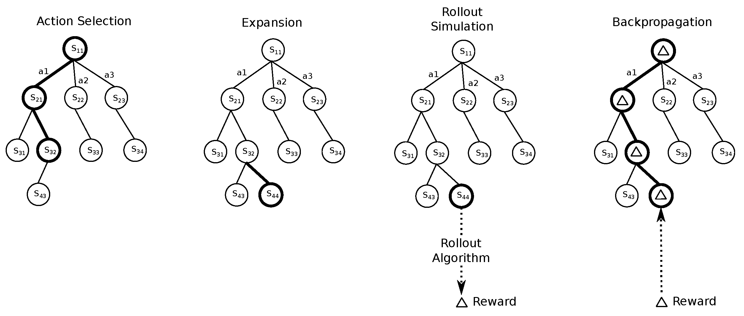
Monte Carlo Tree Search (MCTS) is an online planning method that evaluates the available actions starting from the current state using Monte Carlo simulations. When MCTS is used for Multi-agent Markov Decision Process (MMDP) problems, the search evaluates the cross-product of the sets of actions available to each agent. This is one of the main limitations of MCTS when applied to MMDP. Decoupled-MCTS aims to solve this by evaluating each agents’ set of actions separately. As seen in Figure 2, in decoupled-MCTS, nodes have a set of actions for each agent, in contrast to MCTS, where nodes have a set of joint actions composed of cross-product of all agents’ actions. In the back-propagation step, all individual actions of agents that are selected at that simulation are updated with the same reward.

5.2. Decoupled-MCTS

In multi-agent planning, the complexity of the problem increases exponentially in terms of the number of agents. Decoupled-MCTS tackles this problem by planning for each agent separately. In the planning phase, each agent becomes the part of the environment from the perspective of the planner agent. All agents are both planner and also part of the environment. They collectively plan using the same simulation runs. In the beginning, each agent would be a noise to other agents, but as the agent converges to a behavior, each agent has a chance to adapt to other agents.

Each agent runs a single agent MCTS planning. In the general game-playing domain, this approach works well when the deterministic action selection algorithm is used [2]. All agents get different rewards given the state for these problems. One common example would be zero-sum games, where at each state the sum of the agents’ rewards is 0. Although decoupled-MCTS is not the only method, it works well as it reduces the exponential complexity.

Cooperative multi-agent problem is a subset of the general game-playing problem. The main difference is that all agents share the same reward and aim to optimize the same performance. This difference has a big effect on the performance of decoupled-MCTS when deterministic action selection policy is used. Due to this limitation, we used stochastic action selection policies, which solve the action synchronization problem where statistics of first combinations of actions are fixed at the beginning (see Section 5.2.1).

There are two possible representations for decoupled-MCTS: (1) single search tree and (2) separate search tree. Single search tree differs from single agent MCTS with the representation of actions. At each state node, we have the list of actions available to each agent with their respective statistics and next nodes, as seen in Figure 2. At each action selection, the method selects an action for each agent separately using the statistics, but it expands and moves on the same tree as if it was a single agent MCTS. Separate search tree differs from single search tree by maintaining different search trees for each agent. We have a single agent MCTS search tree for each agent, but action selection and back-propagation is driven by the simulation shared by all agents, as seen in Figure 3. The main advantage of separate search tree is distributed planning where each search tree can be distributed to different computation resource and exchange simulation data as required. Separate search trees also maintain different agent states relevant for Dec-MDP problems that is not in the scope of this paper. However, in this paper, we used the single search tree because we were able to fit search trees in memory and gain efficiency when we combined it to create a search tree over joint action space (see Section 5).

At each planning step, decoupled-MCTS obtains the initial state and constructs a search tree starting from that state. The search tree construction is driven by the simulations and each simulation adds a new node. Nodes contain states, lists of actions and next nodes reachable from each action. Nodes also contain different statistics of the actions to use in an action selection algorithm. The main difference between MCTS and decoupled-MCTS is the representation of actions in search nodes. A decoupled-MCTS node has a list of actions for each agent with the relevant statistics. As a result of this change, decoupled-MCTS runs its selection and back-propagation steps for each agent on their action lists.

Decoupled-MCTS modifies the action selection and back-propagation steps of the MCTS algorithm. The Algorithm 1 presents the main planner that returns the selected set of actions for the given state. The root node is created at the beginning of the algorithm. At each simulation; a new node is added to the tree with EXPAND algorithm, the simulation is run to termination with ROLLOUT algorithm and when the simulation is terminated, BACK-PROPAGATE algorithm updates the statistics of the actions selected during the expansion using the accumulated reward. Finally, the actions of agents having the maximum expected reward are returned.

Algorithm 1 Decoupled Monte Carlo Tree Search

Require:$state$ is the current state Ensure:$action$ is the list of actions   function PLAN($state$)     $root\leftarrow {}_{\mathrm{CREATENODE}}\left(state\right)$     for $i\leftarrow 1\mathrm{to}numSimulations$ do         $leaf\leftarrow {}_{\mathrm{EXPAND}}\left(root\right)$         $reward\leftarrow {}_{\mathrm{ROLLOUT}}\left(leaf\right)$         ${}_{\mathrm{BACKPROPAGATE}}(leaf,reward)$     end for     for $i\leftarrow 1\mathrm{to}numAgents$ do         $actio{n}_i\leftarrow {}_{\mathrm{MAX}}(root.A_i)$     end for     return $action$ end function

The Algorithm 2 shows the expansion of the search tree until a leaf node is reached. The main difference of this algorithm from MCTS is that we select an action ($SELECT$) for each agent using the statistics of the actions. The algorithm moves to the next node or leaf node by running the selected actions on the simulation. When a leaf node is reached a new node is created and connected to the leaf node. When the simulation is terminated, the back-propagation starts. The Algorithm 3 shows how the reward is back-propagated to the nodes that are visited during the current simulation. It starts from the leaf node and updates the statistics of the selected actions with rewards collected after that node. The same reward updates the selected actions of the agents at each node.

Algorithm 2 EXPAND algorithm that traverses the search tree using the statistics of the nodes

Require:$node$ is a node of search tree Ensure:$leaf$ is the leaf node reached by expanding the tree   function EXPAND($node$)     while $\neg {}_{\mathrm{LEAF}}\left(node\right)$ do         for $i\leftarrow 1\mathrm{to}numAgents$ do            $actio{n}_i\leftarrow {}_{\mathrm{SELECT}}(node.A_i)$         end for         $s_{next}\leftarrow {}_{\mathrm{SIM}.\mathrm{STEP}}(node.s,action)$         $node\leftarrow {}_{\mathrm{GETNODE}}\left(s_{next}\right)$     end while     return $node$ end function

Algorithm 3 BACK-PROPAGATE algorithm that updates the value of the nodes traversed during the simulation

Require:$node$ is the leaf node where back propagation starts Require:$rwd$ is reward collected as a result of rollout   function BACKP-ROPAGATE($node,rwd$)     while ${}_{\mathrm{VALID}}\left(node\right)$ do         ${}_{\mathrm{UPDATE}\mathrm{VALUE}}(node,rwd)$         $node\leftarrow {}_{\mathrm{PARENT}}\left(node\right)$     end while end function

5.2.1. Action Synchronization Problem

In decoupled-MCTS, if the action selection policy is deterministic, the initial selection of actions generates a limited number of possible combinations to be evaluated by the simulations. As the number of agents and the number of actions increase, the difference becomes larger. This is a huge limitation that hinders the performance of deterministic policies. We showed that the stochastic action selection policies outperformed the deterministic ones due to this problem.

We used a matrix game, the climbing reward structure of which is shown in Figure 4 for illustrative purposes. There are two agents and each agent has three actions. In decoupled-MCTS, each agent has a table to keep the statistics of each action. Since the matrix game is a single-step planning problem, a table is used instead of a search tree. Note that the action selection is random until all actions are selected at least once. Let us assume that agent 1 chooses $B_1$, $B_2$, and $B_3$ actions and agent 2 chooses $A_2$, $A_3$, and $A_1$ for the first three simulations, respectively. In other words, $\langle B_1,A_2\rangle$, $\langle B_2,A_3\rangle$, and $\langle B_3,A_1\rangle$ action combinations are selected in the first three simulations. According to these selections, the action values are updated as follows: $B_1=-30$, $A_2=-30$, $B_2=6$, $A_3=6$, $B_3=0$, and $A_1=0$. Since each action has some statistics, the next actions are selected based on them. However, a problem arises due to the shared reward. The first selected combinations are synchronized such that their statistics are updated together. For example, when we use UCB1 deterministic action selection policy, agent 1 selects $A_3$ and agent 2 selects $B_2$ since they have the highest UCB1 values. After these actions are selected for some time, the UCB1 explores other actions; agent 1 chooses $A_1$ and agent 2 chooses $B_3$ since they have the second highest values. Finally, agent 1 explores $A_2$ and agent 2 explores $B_1$. As is seen from the action selection pattern, the action combinations that are considered by decoupled-MCTS only consist of the first combinations that are created randomly. Therefore, for that problem, the algorithm only considers three joint action combinations ($\langle B_1,A_2\rangle$, $\langle B_2,A_3\rangle$, and $\langle B_3,A_1\rangle$) out of nine possible combinations.

The action synchronization can affect performance in a limited way, depending on the reward structure of the problem. If some combinations of actions result in the same reward, the UCB1 (or any deterministic action selection policy) can randomize the action selection for actions having the same statistics. It can arise directly from the regularities in the reward structure (similar to the attainable matrix game in Figure 4) or from a specific exploration term that equalizes the UCB1 values of the actions at some stage. In the experiments section, we show that the effect of regularities and exploration term on the performance was limited, and deterministic action selection policies performed worse, compared to stochastic action selection policies.

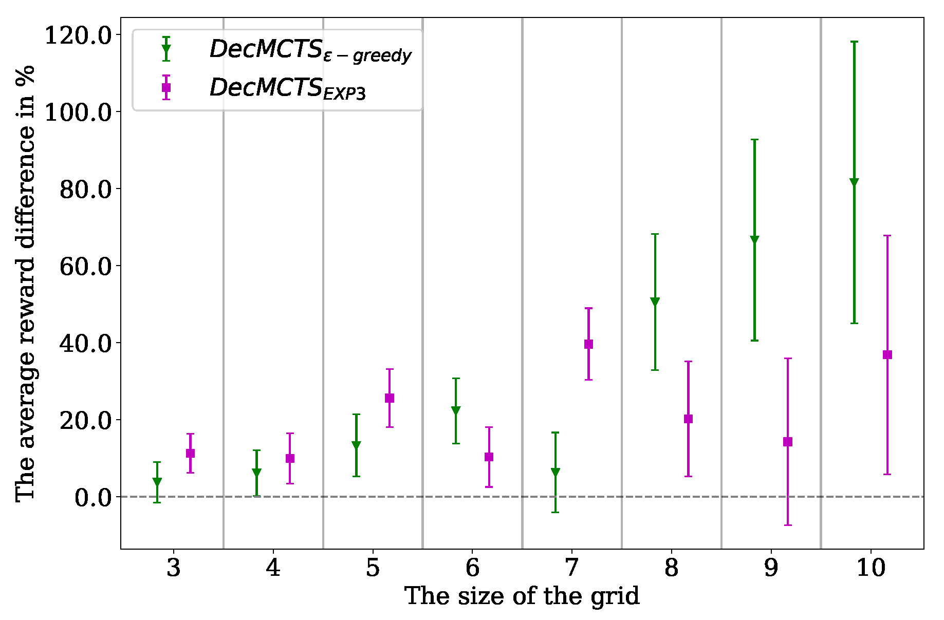
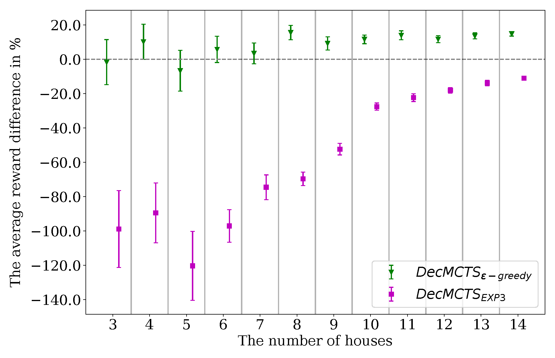
We evaluated two well-known stochastic selection policies: $ϵ$-greedy and EXP3 in the experiments. Although $ϵ$-greedy is simple and lacks good analytical regret boundaries, it performed better than EXP3 in most of the experiments. We observed that the weight iteration step of EXP3 grew boundlessly and equalized all weights at a very high value in our experiments. We normalized and set a maximum weight value to address this issue, but EXP3 was still behind of $ϵ$-greedy. We also found it harder to optimize the exploration parameter of EXP3 compared to $ϵ$-greedy.

5.2.2. Coordination Problem

When using centralized planning with joint actions, the selected joint action ensures the coordination of the actions. However, in the case of decoupled planning, where each agent evaluates its own actions, there is no mechanism to ensure the coordination of actions. Considering the problem, having the attainable reward structure given in Figure 4, the expected values of actions $A_1$ and $A_3$ are the same for agent 1, and, similarly, the expected values of actions $B_1$ and $B_3$ are the same for agent 2 under uniform action selection. However, if their selection of actions is not coordinated, they may get the reward of 0, due to the selection of $\langle B_3,A_1\rangle$ or $\langle B_1,A_3\rangle$ action combinations.

Considering the problem having the penalty reward structure shown in Figure 4, the uncoordinated selection may be penalized. In these cases, the explorations on the action space make these actions unfavorable since their expected values are very low, due to the high penalty values.

This coordination problem is studied in [1] in the independent reinforcement learning domain. Decoupled-MCTS handles each action selection at each node as an independent multi-armed bandit problem. Therefore, the results derived for game matrices in [1] are valid for the action selection in decoupled-MCTS. They show that an exploration strategy with a gradually increasing exploitation converges to an equilibrium. However, the independent learners approach suffers from miscoordination in high penalty cases [38]. In this paper, we propose an improvement on decoupled-MCTS to address the coordination problem in Section 5.3. The method solved the miscoordination by creating a single search tree over a subset of joint actions. The statistics collected in decoupled-MCTS were used for the pruning of joint actions.

5.3. Combined Decoupled Monte Carlo Tree Search

In decoupled-MCTS, we have a coordination problem where agents take actions without knowing which actions were taken by their teammates. Although we have this information, we do not keep or use it in the planning stage because we want to reduce the complexity of the planning. To solve this problem, we propose an improvement over the decoupled-MCTS method. We used decoupled planning to reduce the number of actions available at each node. Once, we completed the decoupled planning, we had good estimations of individual actions of agents. We used this information to construct a search tree over joint actions, but we did not construct all joint actions that would be intractable. We chose joint actions based on the value calculated in decoupled-MCTS planning. Then, we ran another planning stage on this combined search tree using UCT, but we did not add any new nodes to the tree. We were walking on the tree and updating the values of the nodes using rewards collected from new simulation runs. In this way, we improved the performance of overall planning by fine-tuning the joint action evaluations which we might have missed during decoupled planning.

In Figure 5, we show how the decoupled-MCTS search tree was used to construct one new search tree having joint actions. In this simple example, we assumed that nodes were created by running five simulations (sum shows the sum of the collected reward and n shows the number of visits). There were two agents with actions: $A_0$, $A_1$, and $B_0$, $B_1$. If we chose actions based on the current decoupled evaluations, agent 1 would choose $A_1$ and agent 2 would choose $B_0$.

The method uses the statistics from decoupled-MCTS to decide how actions are going to be selected for combining. We sorted individual actions by their selected statistics and chose them to be part of a joint action one by one randomly. This reduced the complexity such that we did not need to construct all possible joint actions. If we used the average cumulative reward as a statistic, in Figure 5, we chose $A_1$ and $B_0$ as the first candidate. Then, to generate the next joint action, we replaced $B_0$ with $B_1$ and kept the $A_1$ as it is. For that example, we randomly chose Agent 2 to update. After the joint actions were selected we calculated their statistics by summing the cumulative rewards of individual actions and dividing that by the total visits to individual actions. The joint action $A_1$, $B_0$ has $4.83$ and $A_1$, $B_1$ had $4.8$ as the cumulative reward. This ensured that the evaluations of individual actions were used to estimate the cumulative reward of the joint action. We set the visit count to 1. In this way, we could incorporate the statistics of individual actions to preset the initial action selection. However, because we set the visit count to 1, we gave very small weight to our initial evaluation.

We limited the number of selected joint actions by the sum of the agents’ actions to keep the total number the same as the decoupled one. For example, if one agent had 4 different actions and another agent had 3 different actions, we chose 7 different joint actions from 12 available joint actions. For the example in Figure 5, we chose two joint actions instead of four for illustrative purposes.

Action Combination Strategies

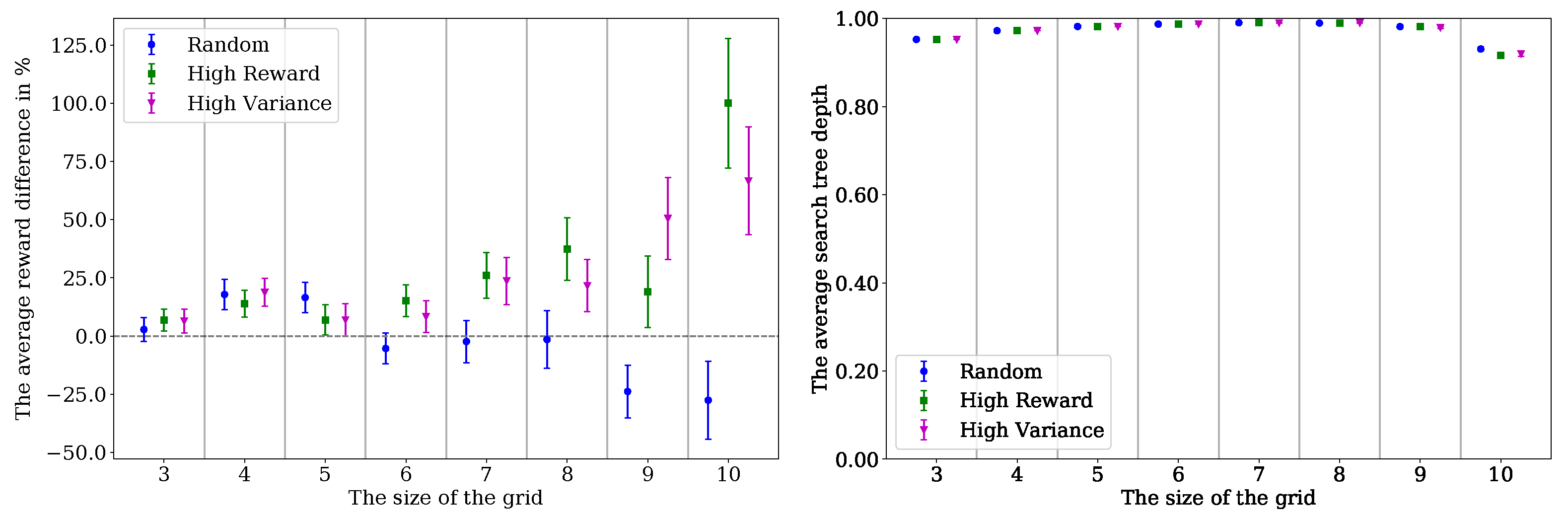
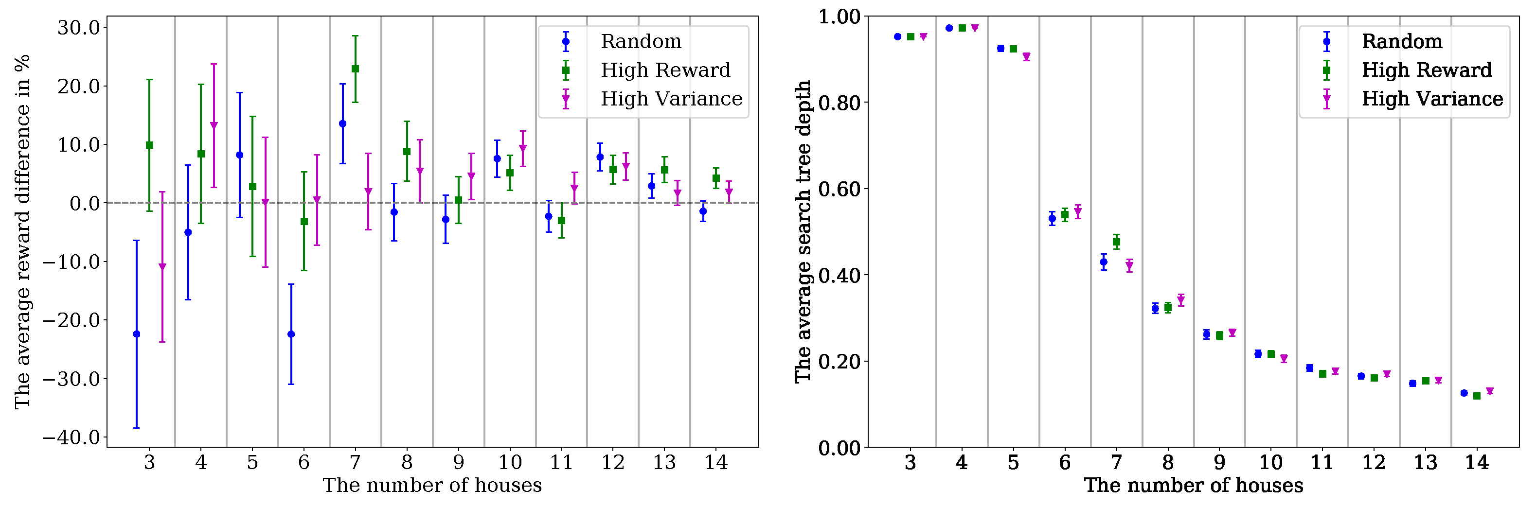
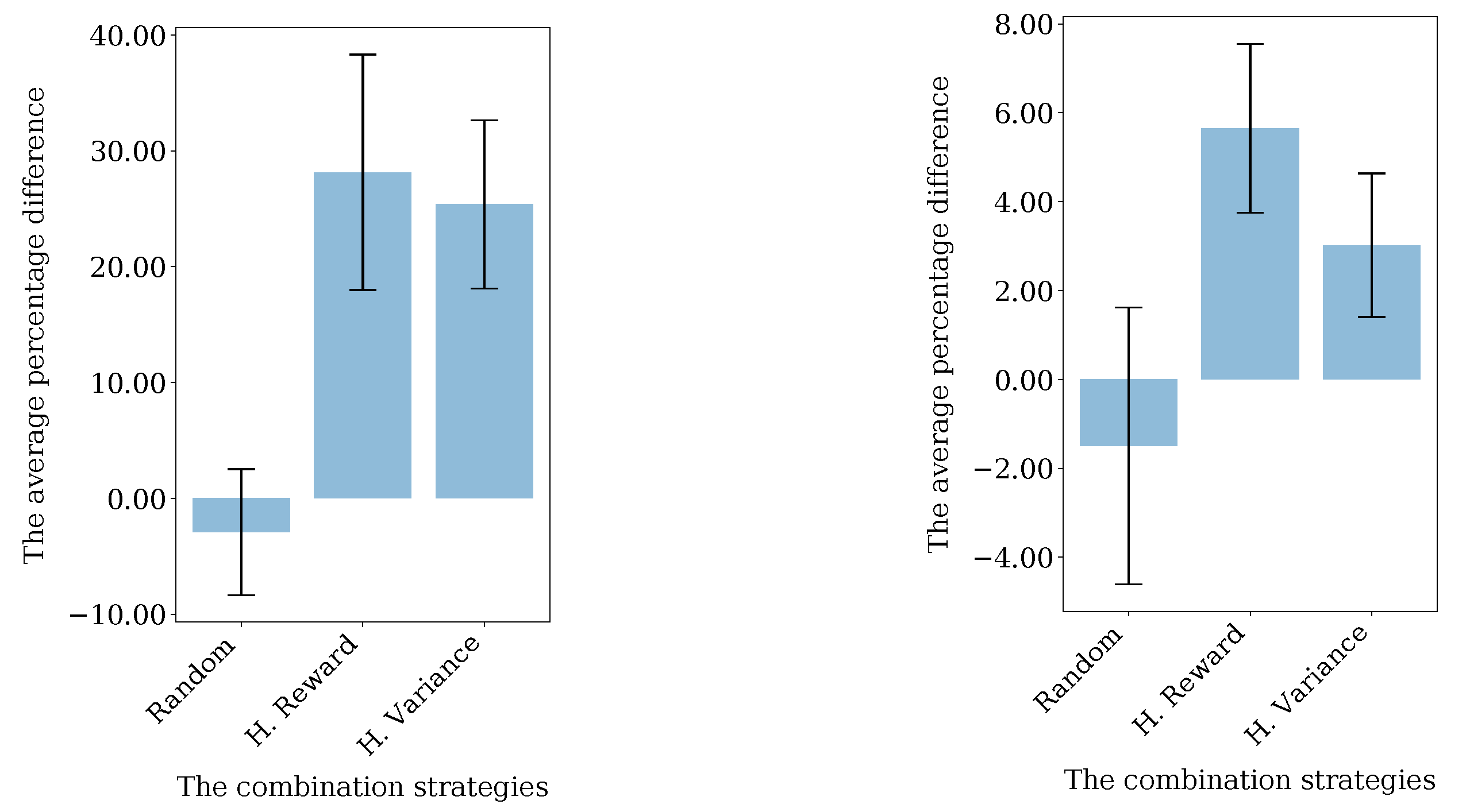
When we collected statistics for individual actions, we used this data to select joint actions. The statistics of the actions could be used in many ways. We proposed two strategies for the combination of joint actions: (1) using the reward, and (2) using the variance of reward. The strategy of using actions with high expected rewards aimed to reevaluate the best actions to reduce the effect of miscalculation. This would reduce the uncertainty introduced due to miscoordination. However, it would not fix the problem of actions severely penalized due to miscoordination. The strategy of using actions with high reward variance addressed that problem. If an action was affected by miscoordination, we expected its variance to be higher than others. When we constructed a joint action from actions with high variance, we gave a new chance to these actions to be evaluated without the uncertainty introduced by other agents. In Section 6.2, we evaluate these strategies with different problems.

6. Results

6.1. The Evaluation of Action Selection Policies

We evaluated the performances of different stochastic action selection policies in decoupled-MCTS. For evaluation, we used cooperative repeated matrix games and MMDP problems from the literature. The best policy was determined by comparing the cumulative average rewards.

6.1.1. Repeated Matrix Games

The repeated matrix games are single-state MMDP problems without action uncertainty. Their reward function depends only on the actions taken. Although they do not have importance in terms of application, they provide an illustrative example. We used two repeated matrix games from the literature [1,38] to study the performance of the action selection policies. They present a challenging problem for independent planners where agents do not know the other agents’ plans. They also have sub-optimal Nash equilibria. Although we observed that decoupled-MCTS could converge to a sub-optimal Nash equilibrium, stochastic action selection policies outperformed deterministic ones.

Experimental Setup

We used the penalty and climbing matrix games, as seen in Figure 4. We replaced k in penalty problem with different values to study the effect of the penalty amount on the performance. Each repeated matrix game was tested with an episode length of 10. For each decision-making step, we ran 500 simulations. The results were provided over 100 runs.

In addition to the matrix games from the literature, we constructed two more matrix games to better illustrate the effect of action synchronization and action combination problems in Figure 6. The random game matrix had randomly unique reward values. The values were less than one for all action combinations, except the reward at $A6\times B6$. We set the reward of one of the action combinations to 10 to set an optimal action with a clear high reward value. The negative penalty game matrix is an extended version of penalty matrix (see Figure 4). We further added penalties and set them to a unique random value less than −100.

We compared $UCB1$, $EXP3$, and $ϵ-greedy$ action selection policies in decoupled-MCTS. The exploration constant of $UCB1$ was set to the difference between maximum and minimum reward, as suggested in  [33]. The $\gamma$ and $ϵ$ parameter of $EXP3$ and $ϵ-greedy$ selection algorithms were selected by running experiments between 0 and 1. The parameters were searched with a $0.01$ increment. We also did not use raw reward for the $EXP3$ action selection policy. The rewards were used as exponential terms in the probability calculation and that resulted in an intractable calculation when rewards were large. To solve that problem, we scaled the reward to a value between 0 and 1. We used $UCB1$ to provide a baseline for deterministic action selection policies.

Results

We present the average cumulative reward for each policy in

Table 1. The performance of decoupled-MCTS with different action selection policies.

	${\mathit{DecMCTS}}_{\mathit{UCB}1}$	${\mathit{DecMCTS}}_{\mathit{EXP}3}$	${\mathit{DecMCTS}}_{\mathit{ϵ}-\mathit{greedy}}$
Climbing	$59.00\pm 0.96$	$49.53\pm 0.18$	$68.34\pm 0.89$
Penalty k = 0	$75.34\pm 1.35$	$93.82\pm 0.77$	$99.72\pm 0.16$
Penalty k = −25	$36.25\pm 1.46$	$44.81\pm 1.85$	$70.82\pm 1.30$
Penalty k = −50	$35.00\pm 1.19$	$22.46\pm 2.60$	$58.44\pm 1.35$
Penalty k = −75	$34.22\pm 1.63$	$19.72\pm 0.07$	$47.86\pm 1.42$
Penalty k = −100	$30.90\pm 1.49$	$19.70\pm 0.11$	$43.84\pm 1.20$
Random	$55.52\pm 1.41$	$88.08\pm 1.03$	$87.86\pm 0.91$
Negative Penalties	$-83.88\pm 10.75$	$-53.34\pm 8.41$	$11.20\pm 4.71$

. The results are provided with standard error. The optimal value of the climbing game matrix was 110, penalty was 100, random was 100, and negative penalties was 100. We observed that the baseline action selection policy ($UCB1$) outperformed $EXP3$ for some of the penalty game matrices and the climbing one. Contrary to our expectations, it did not suffer from action synchronization or coordination problems at the level we expected. When we investigated these problems, we saw that some action combinations resulted in the same reward. Some actions had a reward of 0 and some had symmetric values. When these conditions were met, the action selection was randomized for the actions. That randomization helped to loosen the action synchronization problem.

We investigated the performances for extended matrix games (see Figure 6) for random and negative penalties. As expected, $UCB1$ suffered from action synchronization problems in both game matrices. The reward structures in these game matrices did not help the deterministic action selection policies to randomize its selection. The $EXP3$ and $ϵ-greedy$ methods were not affected severely. Although there was a small performance loss, this could be attributed to the increase in the complexity of the problem, due to the increase in the number of actions. We saw that $ϵ-greedy$ outperformed $EXP3$ in all problems. The performance difference became bigger as the complexity of the problem increased.

In Figure 7, we present the average cumulative reward over the parameters of the action selection policies for penalty k = −100 game matrix. As the parameter value became closer to 1, $ϵ-greedy$ and $EXP3$ made more uniformly random action selections. In other words, they were exploring more. As the exploration increased, the action selection policies converged to the 20 sub-optimal Nash equilibrium. The results for the best parameters are reported in Table 1 and should be evaluated with that information. We observed that $0.1$ was the best parameter for the $ϵ-greedy$ action selection algorithm. An exploration parameter as low as $0.1$ for $ϵ-greedy$ was not feasible for any reasonable problem. However, we could attribute this performance to the deterministic nature of repeated game matrices. It helped exploitative methods to perform better. If the algorithm identified the best action in the initial search, the exploitation paid off well, as there was no uncertainty for the evaluation of the actions.

6.1.2. MMDP Problems

We extended our results to Multi-agent Markov Decision Processes (MMDP) to test action selection policies on problems from literature: meeting in the grid [39] and fire fighting [40]. Although these problems were decentralized partially observable problems, we changed them to be centralized and fully observable to model as MMDP.

Experimental Setup

We redefined meeting in the grid and fire fighting problems as MMDP problems. The meeting in the grid problem had two agents that were, initially, positioned at the top left corner and bottom right corner of the grid, as seen in Figure 8. The grid was defined as a square and its size determined the complexity of the problem. The state of the problem was defined as the position of the agents. They could move north, south, east, west, or stay in the current cell. However, actions failed with a probability of 0.4 and when they failed, a random movement was executed. The agents received a reward of 1 when they met in any cell, and 0 otherwise. The horizon of the problem was defined as two times the grid size; for a 3 by 3 grid, the horizon was 6. All agents received the full state of the problem so that every agent knew where the other agent was.

The fire fighting problem had 2 agents and m houses positioned side to side, as seen in Figure 8. Every house had a fire level that denoted whether the house was on fire and the severity of the fire. In our experiments, we used 3 fire levels: 0 being the no fire level and 2 being the severe fire. The state of the problem was defined as the position of the agents and the fire levels of the houses. Agents could move from one house to another in a single time step, even if the houses were far away from each other. If two agents were in a house, the fire was completely extinguished. If there was one agent, the fire level of the house decreased with 0.6 probability. A house’s fire level increased if there was no agent in that house, with different probabilities determined by its current fire level and the fire levels of its neighbors. The reward of the problem was negative of the sum of fire levels so that the agents were penalized for houses that were on fire. The agents could see the fire levels of houses and their positions. In the beginning, the agents started at an out of house location. The horizon was set as two times the number of houses.

We ran different experiments for the different difficulties of problems. For meeting in the grid problem, we tested for different sizes of the grid. For fire fighting problem, we tested for a different number of houses. We kept the number of agents as two for both problems. We ran 2000 simulations at each decision step and results were provided over 100 experiments. We normalized rewards and kept them between 0 and 1 at each step for the $EXP3$ action selection policy. We used different action selection policy parameters for different problems. For meeting in the grid problem, we found $ϵ=0.61$ and $\gamma =0.05$ were the best parameters when we ran experiments between 0 and 1 with an increment of 0.01 for a grid size of 3. We show the change of the performance over the parameter space for meeting in the grid problem in Figure 9. For the fire fighting problem, we found $ϵ=0.33$ and $\gamma =0.15$ were the best parameters when we ran experiments between 0 and 1 with an increment of 0.01 for a problem with 2 agents and 6 houses. We show the change of the performance over the parameters for the fire fighting problem in Figure 9. Although we chose the best-performing parameters for the experiments, we observed that the selection policies were not sensitive to the parameters as there was no significant performance difference between the parameter values in the range of 0.2 and 0.6. We also ran experiments with UCT algorithm to compare the decoupled-MCTS method to centralized planning. The exploration constant of the UCT was set as the difference between the maximum and minimum cumulative rewards.

Results

We present the average performance of $ϵ-greedy$ and $EXP3$ action selection policies against $UCT$ for meeting in grid problem in Figure 10. We report the average performance difference as a percentage. We showed that decoupled-MCTS outperformed the standard centralized planning algorithm (UCT) in different grid sizes. We also showed that the performance difference became bigger as the size of the grid and the horizon of the problem increased. As the grid size became bigger the goal state was positioned deeper. It would take more steps for agents to meet, which resulted in performance degradation for the UCT algorithm. As the number of simulations was the same for each grid size, the search tree created would be shallow for $UCT$ compared to decoupled-MCTS, due to the high branching factor of joint actions.

When we tested the results for statistical significance using Mann–Withney with $p\le 0.05$, we saw that $EXP3$ outperformed $UCT$ method for grid sizes of 3, 5, and 7, and the $ϵ-greedy$ outperformed for grid sizes of 6, 8, 9. However, when we compared $EXP3$ with $ϵ-greedy$, the performance difference was not significant, except for the problem with the grid size 7. Based on these results, we could conclude that the decoupled-MCTS method outperformed the central planning as well and we did not have a winner action selection policy for decoupled-MCTS for meeting in grid problem.

We present the average performance of $ϵ-greedy$ and $EXP3$ action selection policies against $UCT$ for fire fighting problem in Figure 11. We report the average performance difference as a percentage. In comparison to the meeting in grid problem, $UCT$ outperformed decoupled-MCTS with $EXP3$ action selection. As we previously observed with problems having a negative reward, $EXP3$ action selection was severely affected, although we were normalizing the reward to the 0 and 1 range. $UCT$ also had solid performance against decoupled-MCTS with $ϵ-greedy$ action selection when there were few houses and the problem horizon was small. However, as the number of houses increased that also increased the horizon, and the performance of the $UCT$ degraded. Similar to meeting in grid problem, as the problem became complex centralized planning suffered from a shallow search tree. In the case of fire fighting problem, there was no goal state, but the number of houses determined the available actions to the agents. When the number of houses increased, the number of actions of decoupled-MCTS search increased linearly, but for UCT it increased exponentially.

We tested the results for statistical significance using Mann–Withney with $p\le 0.05$. We saw that $UCT$ outperformed $EXP3$ for all problems. This was an unexpected result, since we expected a decrease in the performance of $UCT$ as the problem complexity increased, but we saw that $EXP3$ was affected by negative rewards. The $ϵ-greedy$ outperformed $UCT$ for problems with houses from 10 to 14. Similarly, $ϵ-greedy$ had a higher reward than $EXP3$ for all problems. Based on the results, we could conclude that decoupled-MCTS with $ϵ-greedy$ action selection outperformed centralized planning when the complexity of the problem increased. Finally, we stated that $ϵ-greedy$ was better than $EXP3$ action selection policy for decoupled-MCTS.

6.2. Coordination Experiments

We evaluated combined decoupled-MCTS with game matrices and MMDP problems. We showed how the performance of decoupled-MCTS was affected by miscoordination. We used problems that had high miscoordination penalties and ones that did not. We evaluated different joint action combination strategies and compared with the best action selection policy of decoupled-MCTS, specifically $ϵ-greedy$.

6.2.1. The Evaluation of Joint Action Combination Strategies

We evaluated two different joint action combination strategies: (1) high reward and (2) high variance. In addition to these strategies, we also evaluated the random combination strategy as a baseline.

Experimental Setup

We had two sets of experiments: repeated matrix games and MMDP problems. We used penalty and climbing repeated matrix games from Figure 4 and also their extended versions from Figure 6. In addition to repeated matrix games, we used meeting in grid and fire fighting MMDP problems. The MMDP problems did not have artificial miscoordination. We aimed to provide an evaluation of general MMDP problems. We used decoupled-MCTS with $ϵ-greedy$ action selection with 500 simulations for repeated game matrices and 2000 simulations for MMDP problems. We selected individual actions using an action combination strategy and combined them to create a search tree of joint actions. Finally, we walked on the combined search tree with the same number of simulations. The results were provided over 100 runs. We report the results with the best performing $ϵ$ parameter, which was searched between 0 to 1 with an increment of 0.01 for repeated game matrices problem. For MMDP problems, we used the best performing $ϵ$ parameter that was determined in Section 6.1.2.

Results

The repeated matrix game results are presented in

Table 2. The performance of combined decoupled-MCTS with different action combination strategies.

	Random	High Reward	High Variance	${\mathit{DecMCTS}}_{\mathit{ϵ}-\mathit{greedy}}$
Climbing	$91.77\pm 0.77$	$81.03\pm 0.92$	$96.37\pm 0.76$	$68.34\pm 0.89$
Penalty k = 0	$100.00\pm 0.00$	$100.00\pm 0.00$	$100.00\pm 0.00$	$99.72\pm 0.16$
Penalty k = −25	$96.92\pm 0.51$	$85.90\pm 1.16$	$98.98\pm 0.28$	$70.82\pm 1.30$
Penalty k = −50	$88.34\pm 0.87$	$75.38\pm 1.23$	$91.86\pm 0.78$	$58.44\pm 1.35$
Penalty k = −75	$79.08\pm 1.22$	$64.42\pm 1.45$	$81.44\pm 1.08$	$47.86\pm 1.42$
Penalty k = −100	$69.56\pm 1.18$	$59.32\pm 1.47$	$74.16\pm 1.44$	$43.84\pm 1.20$
Random	$91.45\pm 0.79$	$98.88\pm 0.30$	$98.41\pm 0.37$	$87.86\pm 0.91$
Negative Penalties	$36.18\pm 1.62$	$47.52\pm 1.28$	$44.64\pm 1.19$	$11.20\pm 4.71$

with standard error. We show that the combined decoupled-MCTS method with different action combination strategies outperformed the decoupled-MCTS statistically significantly when tested with Mann–Withney ($p\le 0.05$). When we compared different action combination strategies, we observed that high variance strategy outperformed highest reward for all problems with negative penalties, except random and negative penalties problems. This difference was statistically significantly when tested with Mann–Withney ($p\le 0.05$). These two problems had more actions than the problems taken from the literature: $8\times 8=64$ joint actions compared to $3\times 3=9$. Although the high reward combination strategy outperformed the high variance, the difference was not significant. We concluded that as the number of available actions increased the advantage of choosing the actions having the high reward variance decreased, even for problems having a penalty for miscoordination.

We present the performance of combination strategies against the decoupled-MCTS method for meeting in grid problems in Figure 12. For meeting in grid problem, the performance difference became bigger as the size of the grid increased. As the size of the grid increased, the goal state moved deeper in the search tree. Every action that took an agent away from the goal reduced performance. The deeper the goal, the probability of moving away from the goal increased. Combined decoupled-MCTS reduced the divergence by increasing the coordination of agents.

We present the performance of combination strategies against the decoupled-MCTS method for fire fighting problems in Figure 13. For fire fighting problem, the performance difference decreased as the number of houses increased. The main reason for the performance degradation was the increase of out-of-tree walk after the combination step. In Figure 12 and Figure 13, we also show the average depth of the created search tree over the problem horizon. We saw that decoupled-MCTS could build a search tree long enough to reach the horizon of the meeting in grid problem for most of the runs. However, the depth of the search tree decreased for fire fighting problem as the number of houses increased. The increase in the number of houses resulted in a harder problem where two agents were not able to completely extinguish the fire. For problems of up to 5 houses, the agents were either able to completely extinguish the fire or able to generate the whole search tree. However, for problems with a number of houses 6 and more, the method was not able to generate an effective search tree up to the problem horizon. When we compared meeting in grid problem with fire fighting, we saw that branching was different. For meeting in grid problem, the branching was the same for all grid sizes, but for fire fighting problem, it increased when the number of houses increased. Another observation was that the different combination strategies did not have a significant effect on search tree depth for both problems.

We present the overall performance of combination strategies in Figure 14. We observed that high reward and high variance strategies improved the performance of $DecMCT{S}_{ϵ-greedy}$ over 25% for meeting in grid problem. Although high reward had higher improvement, it was not significantly better than high variance. For fire fighting problem, the improvement was over 5% for high reward strategy. This was an expected result as we had shown that a shallow search tree limited the performance of the combined methods. However, we saw that high reward outperformed high variance strategy. This difference was due to the importance of coordination. The meeting in grid problem was more sensitive for coordination because it required coordinated movement to meet in a grid. The fire fighting problem generated a reward even if the agents did not act in a coordinated way, which resulted in lower variance. Therefore, it was harder to separate miscoordination variance from noise in the reward.

6.3. Warehouse Problems

In this section, we aimed to compare the proposed methods with the one from the literature on a simplified real-world problem. The warehouse problem is a task allocation problem where robots are executing pickup tasks in a warehouse setting. The warehouse is represented as a graph where robots can move from one node to another, given there is an edge between them, with some uncertainty. All robots start at the depot position. At every time step, new tasks appear at different locations with different costs. The robots get a reward as the negative of the total costs of the tasks that are not yet served. The frequency of each task type for each node is different for every run to simulate high-demand orders at particular locations. The robots pick up orders by moving to the task location. They have a limited capacity and when their inventory is full, they empty it at the depot location.

6.3.1. Experimental Setup

We ran our experiments on the setup, as defined in the work of Claes et al. [8]. We tested with four different warehouse graphs, with different sizes and shapes, as seen in Figure 15. We set the agent capacity to 5. At each decision step, the planning agent used 20,000 simulations for all methods. The results were provided over 30 runs. Every run had the same task schedule and task location for all tested methods. Iterative greedy algorithm [8] was used as a rollout algorithm in all methods because it is the best-performing rollout algorithm.

We compared the following algorithms: $UCT$, $UC{T}_{SA}$, $DecMCT{S}_{ϵ-greedy}$, and $ComDec$$MCT{S}_{ϵ-greedy}^{HR}$. $UCT$ represents the centralized planning over joint actions. The direct application of $UCT$ is intractable for warehouse problems due to exponential action and state space. We restricted the number of actions available at each node to 24 and the number of next states from each action to 20. These numbers were determined empirically to ensure that $UCT$ returned a result using feasible memory. $UC{T}_{SA}$ is the method presented by Claes et al. [8]. $SA$ is the short name for Single Agent. Their method ran a single-agent UCT planning by representing other agents with a greedy algorithm. $DecMCT{S}_{ϵ-greedy}$ is the decoupled-MCTS method that uses $ϵ-greedy$ as the action selection policy. From decoupled-MCTS methods, we evaluated only the $ϵ-greedy$ action selection policy. $ϵ-greedy$ policy is simpler than $EXP3$ and performs better for problems with negative rewards, as shown in Section 6.1. $ComDecMCT{S}_{ϵ-greedy}^{HR}$ is a combined decoupled-MCTS method with high reward combination strategy. We evaluated only high reward combination strategy because it had better performance for MMDP problems in Section 6.1.2. We used $0.7$ as the $ϵ$ value for decoupled-MCTS methods. We determined this value by running 30 experiments for each parameter in the range of 0 and 1 with an increment of $0.05$ for 2 agents small warehouse problem.

6.3.2. Decentralized Planning

The search trees are represented by a single centralized planner. The planner gets the joint state of the problem, runs the decoupled planning, and returns the joint actions. $UC{T}_{SA}$ [8] is a decentralized planing method. However, we ran it in a centralized fashion where we ran the planning one by one for each agent. Finally, we collected the actions from each planner and submitted the joint action.

In the warehouse planning problem, at each decision step, each agent obtains the joint state from the warehouse commissioner, including all tasks in the warehouse. Then, each agent plans using this joint state by calculating a greedy allocation as needed. Our method also supported decentralized planning because joint state was shared at each decision step. Compared to Claes et al., our method ran planning over the search tree for all agents. If we fixed the random seed for each planner, distributed to different computing resources, we were able to run the same simulations for each planner. That ensured each planner would use the same data to represent the teammates. Basically, we would be running the same decoupled-MCTS on each computing resource, but using a single action output from each one. This also opened possibilities to change the teammate search trees to improve the performance, but we did not investigate it in this paper.

6.3.3. Results

We present the average performance of methods with a different number of agents against the method of Claes et al. [8] in Figure 16. The horizontal line at zero represents the method proposed by Claes et al. [8]. We calculated the average reward for each algorithm for each warehouse problem and the number of agents. Then, we calculated the percentage of the difference to the baseline average reward. Finally, we averaged the percentage values over warehouses. We showed that as the number of agents increased the performance gain increased for decoupled methods. This could be attributed to the situation whereby when there were few agents, there would be more tasks in the warehouse that needed to be served. When more tasks waited to be served, modeling other agents with a greedy method resulted in a good approximation of the behavior of other agents. We showed that for problems having more than 5 agents, the $DecMCT{S}_{ϵ-greedy}$ and $ComDecMCT{S}_{ϵ-greedy}^{HR}$ methods improved the baseline by more than 10%. We also showed that the performance of $UCT$ degraded sharply as the number of agents increased. As the number of agents increased, the number of joint actions at each node increased exponentially. As we limited the number of actions, we dismissed useful joint actions from the UCT search tree. The search tree would be evaluating a small subset of joint actions and result in poor performance. When we compared $DecMCT{S}_{ϵ-greedy}$ with $ComDecMCT{S}_{ϵ-greedy}^{HR}$, we did not see a performance difference. For every number of agents, their performances were on par with each other, due to the shallow search tree.

In Figure 17, we present the average percentage difference of methods from the baseline, $UC{T}_{SA}$, over different warehouse problems. We can see that $DecMCT{S}_{ϵ-greedy}$ and $ComDecMCT{S}_{ϵ-greedy}^{HR}$ increased the performance by more than 10% for most of the warehouses. The performance of the decoupled method degraded with the Large warehouse problem. The methods could increase the performance by 5%. This was due to cases where the methods had more tasks that were not served in the Large warehouse because of the size. All agents started at the depot and it took a long time to serve distant tasks. When there were many tasks in the warehouse, the performance of decoupled method became closer to $UC{T}_{SA}$ as the accuracy of representing other agents with the greedy method increased. We also saw how the complexity of the problem affected the centralized planning method. As the complexity increased, the degradation in the performance of $UCT$ increased because of the limits that were necessary to make the method tractable.

Similar to the performance over the number of agents, there was no significant difference between $DecMCT{S}_{ϵ-greedy}$ and $ComDecMCT{S}_{ϵ-greedy}^{HR}$ methods in the results over the warehouses. We show the search tree depth of $ComDecMCT{S}_{ϵ-greedy}^{HR}$ in Figure 17. The search tree depth was calculated as the average search tree depth divided by the horizon of the problem. If the search tree depth could reach the horizon of the problem for every decision step, the value would be 1. The highest depth was for the Small warehouse and it was $0.045$. This value showed how likely the combined method was to walk in the tree and make use of the search tree created. As that value was very low, the combined method was not able to improve the performance over $DecMCT{S}_{ϵ-greedy}$.

We present the average time spent per decision step in Figure 18. We saw that all methods linearly scaled with the number of agents, although the complexity of the problems increased exponentially with the number of agents. We used MCTS for each agent in $DecMCT{S}_{ϵ-greedy}$, and we saw that it increased the complexity linearly and was similar to the $UC{T}_{SA}$. $UCT$ method was slowing down faster than the other methods as the number of agents increased, but its trend was linear, because we limited the branching of the search tree. Another interesting observation was that the running time was mostly dominated by the iterative greedy rollout algorithm. This effect was higher for problems where the task number was high, such as the Large warehouse.

7. Conclusions

We propose a new decoupled planning algorithm (decoupled-MCTS) for cooperative multi-agent planning problems. The proposed method improves the scalability of Monte Carlo Tree Search by decoupling the agents in online planning. Decoupled-MCTS generalizes the decoupled-UCT algorithm to cooperative multi-agent planning. Although decoupled-UCT is used in cooperative problems, it is used without a reference to its limitations.

We present the action synchronization problem in decoupled-MCTS approaches for cooperative problems. When the action selection policy of MCTS is deterministic, a limited number of action combinations are evaluated. We address this issue by proposing stochastic action selection policies. We showed that $ϵ$-greedy action selection policy has the best performance for different problems, such as matrix games and MMDP problems.

We present miscoordination as another limitation of decoupled-MCTS. It is best illustrated when there is a penalty if the agents do not coordinate their actions. We propose a combination approach to address the coordination problem. We analyzed and showed when our combination method was most useful. The combined method improved the decoupled-MCTS significantly when the search tree was not shallow.

We compared our method with another decoupled task allocation method in the warehouse commissioning problem. Our method performed over 10% percent better than the existing method. Our method does not need a greedy rollout algorithm to represent the behaviors of other agents. This increases the applicability of our method.

In this study, we focused on the performance comparison of different stochastic selection policies in different types of problems and reported significant improvements. However, we showed an empirical evaluation of decoupled-MCTS and its combined version. In the future, we aim to further investigate the selection policies in terms of Nash-equilibrium.

References

1. Claus, C.; Boutilier, C. The dynamics of reinforcement learning in cooperative multiagent systems. AAAI/IAAI 1998, 1998, 746–752. [Google Scholar]
2. Finnsson, H.; Björnsson, Y. Simulation-Based Approach to General Game Playing. AAAI 2008, 8, 259–264. [Google Scholar]
3. Shafiei, M.; Sturtevant, N.; Schaeffer, J. Comparing UCT versus CFR in simultaneous games. In Proceedings of the IJCAI-09 Workshop on General Game Playing (GIGA’09), Pasadena, CA, USA, 11–27 July 2009; pp. 75–82. [Google Scholar]
4. Teytaud, O.; Flory, S. Upper confidence trees with short term partial information. In Proceedings of the European Conference on the Applications of Evolutionary Computation, Torino, Italy, 27–29 April 2011; pp. 153–162. [Google Scholar]
5. Auger, D. Multiple tree for partially observable monte-carlo tree search. In Proceedings of the European Conference on the Applications of Evolutionary Computation, Torino, Italy, 27–29 April 2011; pp. 53–62. [Google Scholar]
6. Perick, P.; St-Pierre, D.L.; Maes, F.; Ernst, D. Comparison of different selection strategies in monte-carlo tree search for the game of Tron. In Proceedings of the 2012 IEEE Conference on Computational Intelligence and Games (CIG), Granada, Spain, 11–14 September 2012; pp. 242–249. [Google Scholar]
7. Lanctot, M.; Lisỳ, V.; Winands, M.H. Monte Carlo tree search in simultaneous move games with applications to Goofspiel. In Proceedings of the Workshop on Computer Games; Springer: Berlin/Heidelberg, Germany, 2013; pp. 28–43. [Google Scholar]
8. Claes, D.; Oliehoek, F.; Baier, H.; Tuyls, K. Decentralised online planning for multi-robot warehouse commissioning. In Proceedings of the 16th Conference on Autonomous Agents and MultiAgent Systems, Sao Paulo, Brazil, 8–12 May 2017; pp. 492–500. [Google Scholar]
9. Busoniu, L.; Babuska, R.; De Schutter, B. A comprehensive survey of multiagent reinforcement learning. IEEE Trans. Syst. Man Cybern.-Part C Appl. Rev. 2008, 38, 156–172. [Google Scholar] [CrossRef]
10. Dorri, A.; Kanhere, S.S.; Jurdak, R. Multi-Agent Systems: A Survey. IEEE Access 2018, 6, 28573–28593. [Google Scholar] [CrossRef]
11. Goldman, C.V.; Zilberstein, S. Decentralized Control of Cooperative Systems: Categorization and Complexity Analysis. J. Artif. Intell. Res. 2004, 22, 143–174. [Google Scholar] [CrossRef]
12. Bernstein, D.S.; Givan, R.; Immerman, N.; Zilberstein, S. The Complexity of Decentralized Control of Markov Decision Processes. Math. Oper. Res. 2002, 27, 819–840. [Google Scholar] [CrossRef]
13. Littman, M.L.; Dean, T.L.; Kaelbling, L.P. On the complexity of solving Markov decision problems. In Proceedings of the Eleventh Conference on Uncertainty in Artificial Intelligence, Montreal, QC, Canada, 18–20 August 1995; pp. 394–402. [Google Scholar]
14. Panait, L.; Luke, S. Cooperative multi-agent learning: The state of the art. Auton. Agents -Multi-Agent Syst. 2005, 11, 387–434. [Google Scholar] [CrossRef]
15. Lauer, M.; Riedmiller, M. An algorithm for distributed reinforcement learning in cooperative multi-agent systems. In Proceedings of the Seventeenth International Conference on Machine Learning, Stanford, CA, USA, 29 June–2 July 2000. [Google Scholar]
16. Peshkin, L.; Kim, K.E.; Meuleau, N.; Kaelbling, L.P. Learning to cooperate via policy search. In Proceedings of the Sixteenth Conference on Uncertainty in Artificial Intelligence, San Francisco, CA, USA, 30 June–3 July 2000; pp. 489–496. [Google Scholar]
17. Gronauer, S.; Diepold, K. Multi-agent deep reinforcement learning: A survey. Artif. Intell. Rev. 2022, 55, 895–943. [Google Scholar] [CrossRef]
18. Zhang, K.; Yang, Z.; Başar, T. Multi-agent reinforcement learning: A selective overview of theories and algorithms. In Handbook of Reinforcement Learning and Control; Springer: Berlin/Heidelberg, Germany, 2021; pp. 321–384. [Google Scholar]
19. Sunehag, P.; Lever, G.; Gruslys, A.; Czarnecki, W.M.; Zambaldi, V.; Jaderberg, M.; Lanctot, M.; Sonnerat, N.; Leibo, J.Z.; Tuyls, K.; et al. Value-Decomposition Networks For Cooperative Multi-Agent Learning Based On Team Reward. In Proceedings of the 17th International Conference on Autonomous Agents and MultiAgent Systems, Stockholm, Sweden, 10–15 July 2018; pp. 2085–2087. [Google Scholar]
20. Colby, M.; Duchow-Pressley, T.; Chung, J.J.; Tumer, K. Local approximation of difference evaluation functions. In Proceedings of the 2016 International Conference on Autonomous Agents & Multiagent Systems, Singapore, 9–13 May 2016; pp. 521–529. [Google Scholar]
21. Bargiacchi, E.; Verstraeten, T.; Roijers, D.M. Cooperative Prioritized Sweeping. In Proceedings of the 20th International Conference on Autonomous Agents and MultiAgent Systems, Online, 3–7 May 2021; pp. 160–168. [Google Scholar]
22. Oliehoek, F.; Witwicki, S.; Kaelbling, L. A sufficient statistic for influence in structured multiagent environments. J. Artif. Intell. Res. 2021, 70, 789–870. [Google Scholar] [CrossRef]
23. Busoniu, L.; De Schutter, B.; Babuska, R. Decentralized reinforcement learning control of a robotic manipulator. In Proceedings of the 2006 9th International Conference on Control, Automation, Robotics and Vision, Singapore, 5–8 December 2006; pp. 1–6. [Google Scholar]
24. Leottau, D.L.; Vatsyayan, A.; Ruiz-del Solar, J.; Babuška, R. Decentralized Reinforcement Learning Applied to Mobile Robots. In Proceedings of the Robot World Cup; Springer: Berlin/Heidelberg, Germany, 2016; pp. 368–379. [Google Scholar]
25. Best, G.; Cliff, O.M.; Patten, T.; Mettu, R.R.; Fitch, R. Dec-MCTS: Decentralized planning for multi-robot active perception. Int. J. Robot. Res. 2019, 38, 316–337. [Google Scholar] [CrossRef]
26. Amini, S.; Palhang, M.; Mozayani, N. POMCP-based decentralized spatial task allocation algorithms for partially observable environments. Appl. Intell. 2022, 1–19. [Google Scholar] [CrossRef]
27. Czechowski, A.; Oliehoek, F.A. Decentralized MCTS via learned teammate models. In Proceedings of the Twenty-Ninth International Conference on International Joint Conferences on Artificial Intelligence, Yokohama, Japan, 7–15 January 2021; pp. 81–88. [Google Scholar]
28. Tak, M.J.; Lanctot, M.; Winands, M.H. Monte Carlo tree search variants for simultaneous move games. In Proceedings of the 2014 IEEE Conference on Computational Intelligence and Games, Dortmund, Germany, 26–29 August 2014; pp. 1–8. [Google Scholar]
29. Kurzer, K.; Zhou, C.; Marius Zöllner, J. Decentralized Cooperative Planning for Automated Vehicles with Hierarchical Monte Carlo Tree Search. In Proceedings of the 2018 IEEE Intelligent Vehicles Symposium (IV), Suzhou, China, 26–30 June 2018; pp. 529–536. [Google Scholar] [CrossRef] [Green Version]
30. Kearns, M.; Mansour, Y.; Ng, A.Y. A sparse sampling algorithm for near-optimal planning in large Markov decision processes. Mach. Learn. 2002, 49, 193–208. [Google Scholar] [CrossRef]
31. Coulom, R. Efficient selectivity and backup operators in Monte-Carlo tree search. In Proceedings of the International Conference on Computers and Games; Springer: Berlin/Heidelberg, Germany, 2006; pp. 72–83. [Google Scholar]
32. Kocsis, L.; Szepesvári, C. Bandit based monte-carlo planning. In Machine Learning: ECML 2006; Springer: Berlin/Heidelberg, Germany, 2006; pp. 282–293. [Google Scholar]
33. Silver, D.; Veness, J. Monte-Carlo Planning in Large POMDPs. In Advances in Neural Information Processing Systems 23; Lafferty, J.D., Williams, C.K.I., Shawe-Taylor, J., Zemel, R.S., Culotta, A., Eds.; Curran Associates, Inc.: Red Hook, NY, USA, 2010; pp. 2164–2172. [Google Scholar]
34. Auer, P.; Cesa-Bianchi, N.; Freund, Y.; Schapire, R.E. The nonstochastic multiarmed bandit problem. SIAM J. Comput. 2002, 32, 48–77. [Google Scholar] [CrossRef]
35. Slivkins, A.; Upfal, E. Adapting to a Changing Environment: The Brownian Restless Bandits. In Proceedings of the COLT, Helsinki, Finland, 9–12 July 2008; pp. 343–354. [Google Scholar]
36. Auer, P.; Cesa-Bianchi, N.; Fischer, P. Finite-time analysis of the multiarmed bandit problem. Mach. Learn. 2002, 47, 235–256. [Google Scholar] [CrossRef]
37. Audibert, J.Y.; Bubeck, S. Minimax policies for adversarial and stochastic bandits. In Proceedings of the 22nd Annual Conference on Learning, Theory, Montreal, QC, Canada, 18–21 June 2009; pp. 773–818. [Google Scholar]
38. Papoudakis, G.; Christianos, F.; Schäfer, L.; Albrecht, S.V. Comparative evaluation of cooperative multi-agent deep reinforcement learning algorithms. In Proceedings of the Adaptive and Learning Agents Workshop (ALA 2021), Virtual, 3–7 May 2021. [Google Scholar]
39. Bernstein, D.S.; Hansen, E.A.; Zilberstein, S. Bounded policy iteration for decentralized POMDPs. In Proceedings of the Nineteenth International Joint Conference on Artificial Intelligence (IJCAI), Scotland, UK, 30 July–5 August 2005; pp. 52–57. [Google Scholar]
40. Oliehoek, F.A.; Spaan, M.T.; Vlassis, N.A. Optimal and Approximate Q-value Functions for Decentralized POMDPs. J. Artif. Intell. Res. (JAIR) 2008, 32, 289–353. [Google Scholar] [CrossRef] [Green Version]
Figure 1. Monte Carlo Tree Search has four steps: Action selection, expansion, rollout, and back-propagation.
Applsci 13 01936 g001
Figure 2. On the left, the search tree of UCT with the joint actions. On the right, the search tree of decoupled-MCTS with nodes having different set of actions for each agent separately.
Applsci 13 01936 g002
Figure 3. On the left, Decoupled-MCTS with separate search trees for Agent 1 and Agent 2. On the right, the interaction between a simulator and separate search trees in the planning phase.
Applsci 13 01936 g003
Figure 4. Game matrices with different coordination problems: Attainable, penalty, and climbing as presented by Claus et al. [1].
Applsci 13 01936 g004
Figure 5. Combining single agent actions of decoupled-MCTS to create a search tree with joint actions.
Applsci 13 01936 g005
Figure 6. Random (left): A game matrix having an optimal action combination with value 10. Negative penalties (right): A game matrix having high penalties for all action combinations in addition to the original penalty game matrix.
Applsci 13 01936 g006
Figure 7. The average cumulative reward over the action selection policy parameters: ϵ and γ in Penalty k = −100 repeated game matrix. The whiskers show the standard error.
Applsci 13 01936 g007
Figure 8. MMDP Problems. (left) The fire fighting problem. (right) The meeting in grid problem.
Applsci 13 01936 g008
Figure 9. The average cumulative reward over the action selection policy parameters: ϵ and γ in MMDP Problems. (left) The fire fighting problem. (right) The meeting in grid problem. The whiskers show the standard error.
Applsci 13 01936 g009
Figure 10. The average cumulative reward difference in % over different grid size of meeting in grid problem. 0.0 line represents the performance of U C T . The whiskers show the standard error.
Applsci 13 01936 g010
Figure 11. The average cumulative reward difference in % over different number for houses of fire fighting problem. 0.0 line represents the performance of U C T . The whiskers show the standard error.
Applsci 13 01936 g011
Figure 12. The results of combination strategies experiments for meeting in grid problem. (left) The average cumulative reward difference. 0.0 line represents the performance of D e c M C T S ϵ g r e e d y . (right) The average depth of the search tree over the problem horizon. The whiskers show the standard error.
Applsci 13 01936 g012
Figure 13. The results of combination strategies experiments for fire fighting problem. (left) The average cumulative reward difference in %. 0.0 line represents the performance of D e c M C T S ϵ g r e e d y . (right) The average depth of the search tree over the problem horizon. The whiskers show the standard error.
Applsci 13 01936 g013
Figure 14. The results of combination strategies for (left) meeting in grid and (right) fire fighting problem for all problem sizes. The results are averaged over the percentage difference of the strategies from D e c M C T S ϵ g r e e d y . The whiskers show the standard error.
Applsci 13 01936 g014
Figure 15. The warehouse problems from Claes et al. [8]. Green nodes represent depot locations.
Applsci 13 01936 g015
Figure 16. The performance comparison of algorithms in percentage over all warehouse problems. The 0 represents the method of Claes et al. The whiskers show the standard error.
Applsci 13 01936 g016
Figure 17. (left) The average percentage difference of methods from U C T S A over different warehouse problems. (right) The average search tree depth of C o m D e c M C T S ϵ g r e e d y H R . The whiskers show the standard error.
Applsci 13 01936 g017
Figure 18. The average running time per decision step in Large warehouse problem over the number of agents for iterative rollout algorithm. The whiskers show the standard error.
Applsci 13 01936 g018