A Generalized Deep Learning Approach to Seismic Activity Prediction

Abstract

Seismic activity prediction has been a challenging research domain: in this regard, accurate prediction using historical data is an intricate task. Numerous machine learning and traditional approaches have been presented lately for seismic activity prediction; however, no generalizable model exists. In this work, we consider seismic activity predication as a binary classification problem, and propose a deep neural network architecture for the classification problem, using historical data from Chile, Hindukush, and Southern California. After obtaining the data for the three regions, a data cleaning process was used, which was followed by a feature engineering step, to create multiple new features based on various seismic laws. Afterwards, the proposed model was trained on the data, for improved prediction of the seismic activity. The performance of the proposed model was evaluated and compared with extant techniques, such as random forest, support vector machine, and logistic regression. The proposed model achieved accuracy scores of 98.28%, 95.13%, and 99.29% on the Chile, Hindukush, and Southern California datasets, respectively, which were higher than the current benchmark model and classifiers. In addition, we also conducted out-sample testing, where the evaluation metrics confirmed the generality of our proposed approach.

1. Introduction

Earthquakes are considered one of the most dangerous natural disasters, as they can occur without warning. The ratio of deaths caused by earthquakes is above half more than that of other natural disasters [1]. According to the World Health Organization (WHO), earthquakes killed 750,000 people worldwide between 1998 and 2017 [1]. During this period, more than 125 million people were affected by tremors, meaning that they were either injured or lost their houses and valuable properties. In 2020, Americans lost USD 4.4 billion, due to catastrophic earthquakes. Seismic activity prediction is the optimal technique for avoiding earthquake-related economic and human tragedies.

Machine learning (ML) approaches play a pivotal role in prediction and forecasting in various fields, including different disasters, such as floods, earthquakes, and landslides [2,3,4,5,6,7,8]. Significant research has been conducted, using these techniques, to reduce the impact of the aforementioned disasters [3,6,7,9]. These studies have utilized a variety of machine learning approaches, including artificial neural network [5], support vector machine [9], random forest [10], and convolutional neural network [6]. In this work, we consider the seismic activity prediction problem as a binary classification problem, and present a deep neural network model for predicting the occurrence or otherwise of significant seismic activity.

Asim et al. [11] used genetic programming and Ada-boost methods to classify seismic activities in the California region. The authors applied the mentioned methods on only one dataset, and reported accuracy of 78%. An artificial neural network was implemented by Oktarina et al. [5] for earthquake prediction in the Indonesian region, and it calculated the mean square error. Jena et al. [6] studied the Palu region in Indonesia, to identify earthquake-prone areas using cluster analysis techniques. The authors used silhouette clustering, pure locational clustering based on hierarchical clustering analysis, and convolutional neural networks. The approach to the selected region achieved 89% accuracy. Majhi et al. [12] used a moth flame optimized functional link with an artificial neural network to predict seismic magnitude on earthquake catalog data, by considering the mean square error as a metric. Zhang et al. [13] discussed the precursory pattern-based feature extraction method for earthquake prediction in China. The authors used an artificial neural network for earthquake prediction, and reported accuracy of 80%. A different approach was used by Aslam et al. [14] in the northern areas of Pakistan, for the prediction of seismic activity. The authors implemented the support vector machine and hybrid neural network on the targeted area, to predict earthquake occurrence for a period of one month: the maximum accuracy of their models was 79% on one dataset. Al Banna et al. [15] advocated the use of long short-term memory network structure for predicting earthquakes in the Bangladesh region: the authors used hyper-parameters optimization, as well as L1 and L2 regularization, to achieve maximum accuracy of 76%.

From the current literature, we identified that although machine learning models are used to predict earthquake occurrence to varying degree of success, the models mostly rely on data from one region, and there is no generalization in the proposed models. Generalization refers to the concept of the effectiveness (such as higher accuracy, low mean squared error) of a given machine learning model at learning from the given data, and effectively applying the learning to other datasets. The machine learning models proposed for earthquake prediction are not generalized, i.e., the proposed models performed well (to a certain degree) on the given datasets, but their performances on other datasets were either not evaluated or were found lacking: that is to say, the models could not be applied to other datasets/regions.

In this work, a novel methodology for prediction of earthquakes using feature engineering and a deep-learning-based technique is proposed. First, we collected the data for three regions: California, Chile, and Hindukush. The data collection was followed by data cleaning and pre-processing. New features were calculated based on the various seismic laws (such as the Gutenberg–Richter law). The features included the seismic rate of changes, foreshock frequencies, the release of seismic energy, the total time of recurrence, the maximum/minimum relevance, and redundancy. These features were extracted and used as input for our deep learning model. Afterwards, a deep-neural-network-based architecture was proposed, which was evaluated against standard benchmark algorithms, using accuracy, precision, recall, and F1-score.

Unlike previous works, we conducted Out of Sample testing, to validate the generality of the proposed technique. Out of Sample testing means that the model is trained on one dataset, but is evaluated on a different dataset. A better performance on an Out of Sample test reflects that the model is generalized, and can be used for datasets other than the one on which it was trained. The results showed that the proposed deep neural network was more accurate than the other machine learning approaches. This research will aid risk and uncertainty mitigation, for better decision-making regarding earthquake prediction, in various ways.

The rest of this paper is organized in the following manner: Section 2 presents the proposed methodology, including the dataset, feature engineering, the proposed deep neural network architecture, the benchmark algorithms, and the evaluation metrics; the results are presented and discussed in Section 3; Section 4 concludes the work.

2. Methodology

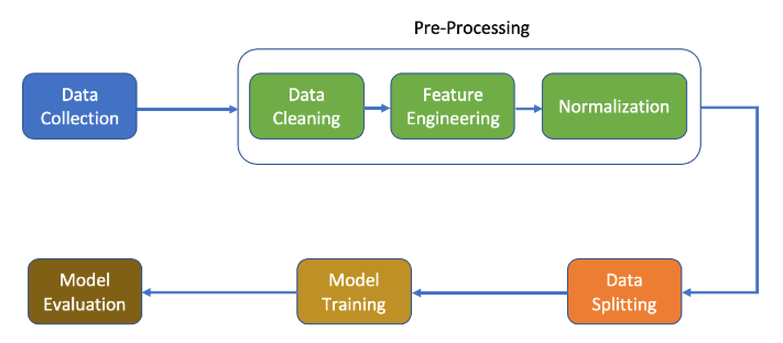
Figure 1 illustrates the workflow of the conducted research. As a first step, the data were collected from various sources, after which the pre-processing was performed. The pre-processing steps included data cleaning, feature engineering, and data normalization. Afterwards, the data were split into training and test sets, and model training was carried out on the training set. Once the training had been performed, and satisfactory results had been achieved on the training set, the model was evaluated on the test data based on the evaluation criterion. In the following, we explain the various phases in detail.

The steps of the proposed methodology are described as follows.

2.1. Data Collection

Earthquakes produces seismic waves, which are recorded in the form of seismograms. Seismograms represent ground motion at a specific location, as a function of time. A phase in seismic waves is the arrival pattern, which is observed in the seismogram: of particular interest are P-waves and S-waves [16]. A seismogram also records the size of an earthquake at its source location (called the epicenter), which is generally referred to as magnitude. Magnitude is a logarithmic measure [16].

Numerous techniques of data acquisition, analysis and filtering in time, frequency, and scale domains exist in the literature [17,18]. In this study, however, we did not use the raw seismograms data: instead, we selected the already-available digital data for three of the most active zones in the globe, for earthquake occurrences. The original seismic activities data were downloaded, from the information provided in the respective articles [9,19,20]. The downloaded data contained the magnitude data. As these three datasets had been used in the existing literature [9,19,20], we also selected the same, for a meaningful comparison. Due to space constraint, the process of data collection from the various sources cannot be explained here, and the reader is referred to the respective sources, which are available at [9,19,20].

Table 1. Description of each dataset.

Region	Total Records	Records after Cut-Off	Label-Yes	Label-No
California	33,543	29,120	4433	24,687
Chile	7656	7590	2002	5588
Hindukush	4350	4274	1379	2971

provides an overview of each dataset.

2.2. Pre-Processing

After obtaining the data from various sources, the data cleaning and feature engineering steps were performed as follows.

2.2.1. Data Cleaning

After obtaining the raw data from the original sources (please refer to [9,19,20]), the data cleaning step was performed. In the data cleaning, the dataset was reviewed for missing values and invalid values. Once it had been ascertained that there were no missing/invalid values, the data were reviewed for cut-off magnitude. The threshold for cut-off magnitude is dependent on the density of the instrumentation in a particular region [9]. As discussed in Asim et al. [9], the cut-off magnitude is $2.6$ for the California region, $3.4$ for Chile, and $4.0$ for Hindukush. Weimer and Wyess [21] have discussed various methodologies for determining the cut-off magnitude; however, in line with the existing literature, we used the Gutenberg–Richter law [9]. The determination of the magnitude of completeness was independent of the Gutenberg–Richter law.

2.2.2. Feature Engineering

The process of extracting new attributes, characteristics, and properties from data is called feature engineering. The main goal of feature engineering is to design/create new features that can be used to improve the performance of the model. The features are engineered based on seismic activities indicators. The features are considered from the available literature. The detailed description about various engineered features is given as follows.

Gutenberg–Richter Law

The Gutenberg–Richter law describes the relationship between the magnitude and the number of earthquakes in a particular region [22]. The Gutenberg–Richter law states that earthquake magnitudes are distributed exponentially as:

$${log}_{10}\left(N\ge m\right)=a-bm;m\ge m_c$$

(1)

Note that N represents the number of earthquakes of magnitudes of at least m, such that $m\ge m_c$, $m_c$ is the threshold magnitude of completeness, b is referred to as the scaling parameter, and a is a constant.

Two different methods—least square regression analysis ($LSQ$) and maximum likelihood ($MLQ$)—were used to calculate the values of a and b. We used both sets of techniques to identify the values of a and b, and we used these values as our features for the machine learning models. The values of a and b were calculated using least square regression, and the maximum likelihood criterion was calculated using Equations (2)–(5) [23].

$$b_{lsq}={\displaystyle \frac{n\left(\sum M_{i}log{N}_i\right)-\left(\sum M_i\sum log{N}_i\right)}{{\left(\sum M_i\right)}^2-n\sum M_i^2}}$$

(2)

$$a_{lsq}={\displaystyle \frac{\sum \left({log}_{10}{N}_i+b_{lsq}{M}_i\right)}{n}}$$

(3)

$$b_{mlk}={\displaystyle \frac{{log}_{10}e}{M_{mean}-M_{min}}}$$

(4)

$$a_{mlk}={log}_{10}N+b_{mlk}\left(M_{min}\right)$$

(5)

Mean of Earthquake Magnitude

The mean of the earthquake magnitude was the mean value of n events, as shown in Equation (6). Prior to any large-scale earthquake, the seismic magnitude is usually rising.

$$M_{mean}=\frac{{\sum }_i{M}_i}{n}$$

(6)

Standard Deviation of b’s Value

The standard deviation of b’s value (${\sigma }_b$) was established by Shi and Bolt [24], and is calculated as shown in Equation (7):

$${\sigma }_b=2.30b^2\sqrt{{\displaystyle \frac{{\sum }_{i=1}^n{\left(M_i-M_{mean}\right)}^2}{n(n-1)}}}$$

(7)

Recurrence Time

The time between two magnitudes of earthquakes equal to or greater than $M^{\prime }$ ($M^{\prime }$ being the value of fixed magnitude) is called the total recurrence time, and is calculated using Equation (8) [9]; it is also called the probabilistic recurrence time ($T_{rec}$).

$$T_{rec}={\displaystyle \frac{T}{{10}^{a-b{M}^{\prime }}}}$$

(8)

Note that T is the length of total time under consideration.

Seismic Rate of Change

In a region, the increase and decrease seismic behavior for two different time intervals is called the Seismic Rate of Change. We calculated the decrease in seismic behavior, using Equation (9) [25]:

$$\beta ={\displaystyle \frac{M(t,\delta )-n\delta }{\sqrt{n\delta (1-\delta )}}}$$

(9)

where n is the number of events, the duration of time is t, and the observed events are $M(t,\delta )$.

To calculate the increase in seismic behavior, we used Equation (10) [26]:

$$z=\frac{R_1-R_2}{\sqrt{{\displaystyle \frac{S_1+S_2}{n_1+n_2}}}}$$

(10)

where $R_1$ and $R_2$ are the seismic rates for two difference intervals, $S_1$ and $S_2$ represent the standard deviation, and $n_1$ and $n_2$ represent the seismic events observed in the two intervals.

Rate of Square Root of Seismic Energy Released

The rate of the square root of seismic energy released over time T was calculated as shown in Equation (11):

$$d{E}^{\frac{1}{2}}=\frac{\sum {\left({10}^{11.8+1.5M}\right)}^{1/2}}{T}$$

(11)

In cases where the release of seismic energy is not possible for a prolonged duration, the abrupt accumulated energy release may result in major seismic activity [27].

Elapsed Time for Last n Seismic Activities

The n number of seismic events to have occurred before $E_t$, as represented in Equation (12) in days, is elapsed time:

$$T=t_n-t_1$$

(12)

Maximum Earthquake Magnitude in the Last 7 Days

This feature is considered an important parameter of seismic events: it means the maximum magnitude recorded in the last 7 days. The mathematical representation is given in Equation (13):

$$X_{max7}=Max\left(M_t\right);t\in \{1,2,....,7\}$$

(13)

Note that $M_t$ is the magnitude of the earthquake observed on day t.

Earthquake Magnitude Deficit

The earthquake magnitude deficit is defined as the difference between the maximum observed magnitude and the maximum possible magnitude defined by $ai/bi$ from the Gutenberg–Richter relationship, and is formulated as shown in Equation (14). Note that $a_i$ and $b_i$ are the parameters of the Gutenberg–Richter relationship, and $Max$ represents

$$\Delta M=Max-max\left(\frac{a_i}{b_i}\right)$$

(14)

2.2.3. Normalization

Data normalization for machine learning models is an essential part of the pre-processing. Normalization is transforming the numeric values to a common scale without wrenching differences from the range of values. The calculated features were normalized using the MinMaxScaler from the scikit-learn library.

Pre-processing is a mandatory step, which is known to have a significant impact on the performance and generalizability of machine learning models [28]: these steps are, as such, required, and cannot be ignored.

2.3. Data Splitting

In machine learning, data splitting is normally utilized for splitting the dataset into training and test sets. Using the “Train/Test split” from the scikit-learn, the datasets were divided into two parts, with 75% of the data being used for training, while the remaining 25% was used for testing.

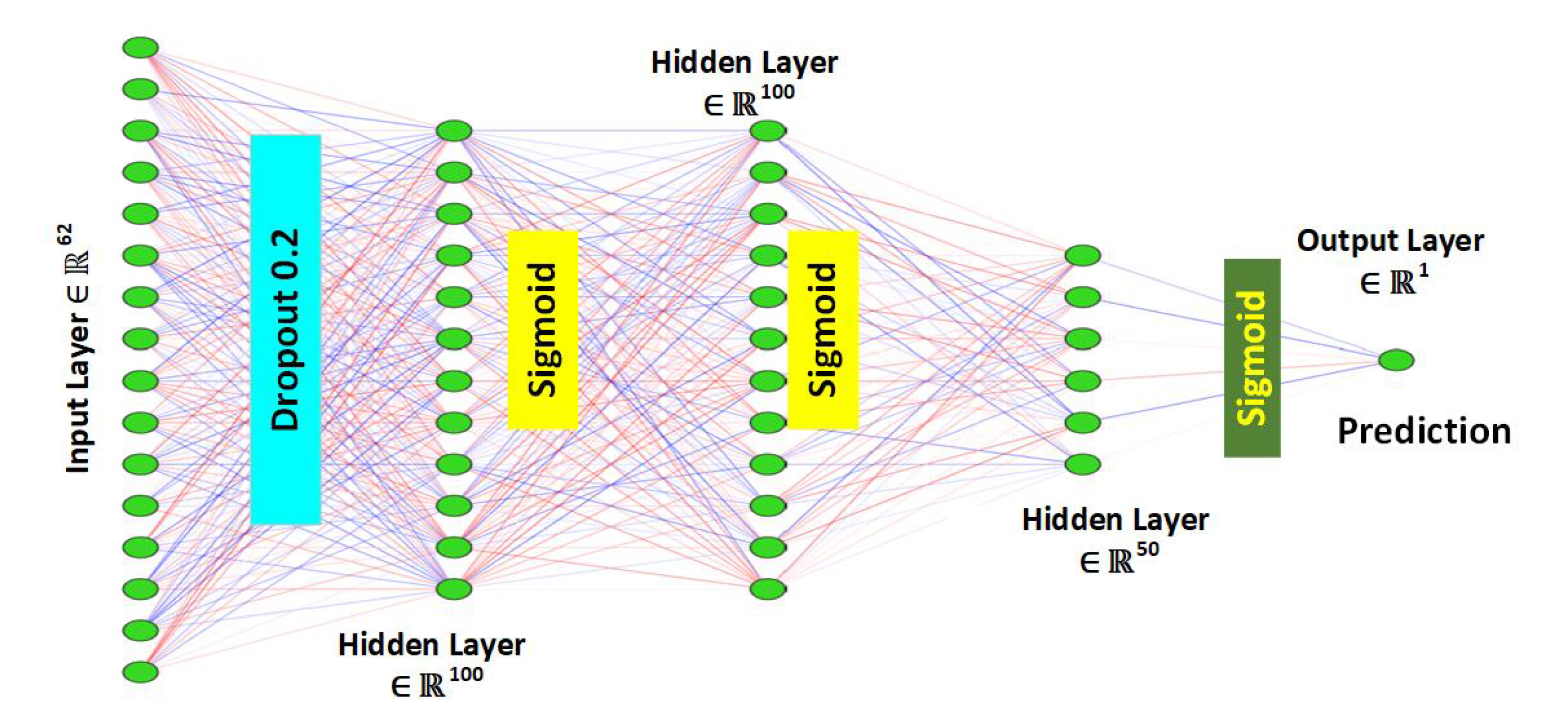
2.4. The Proposed Deep Neural Network Architecture

2.4.1. Layers in the Model

A sequential deep neural network (DNN) model was proposed in this work. The model contained one input layer, three hidden layers, and one output layer for earthquake prediction. The input layer contained 62 neurons, which represented the no. of features. The three hidden layers contained 100, 100, and 50 neurons, respectively, while the output layer comprised a single neuron. The number of layers, and the number of neurons in each hidden layer, were initially selected randomly, and the final values were the ones which provided the optimum results. The sigmoid function was used for all layers except the input layer. The model was implemented in Python 3.7, using Jupyter Notebook as an IDE.

2.4.2. Addressing Over-Fitting

Over-fitting is a common problem in machine learning, and happens when a model does not generalize effectively from observed to unseen data [29]. In order to avoid over-fitting from the data, the dropout $0.2$ was used after the first layer of the model.

2.4.3. Activation Function

The sigmoid function was used as activation and output function in the proposed model. The sigmoid function—also called the logistic function—is mathematically represented as follows:

$$Sigmoid=\frac{1}{1+e^{-x}}$$

(15)

Furthermore, a binary cross-entropy (BCE) [30] as loss function, and “Adam” as an optimizer, were used in the model. The mathematical representation of the BCE is as follows:

$${\displaystyle BCE=-{\displaystyle \frac{1}{N}}\sum _{i=1}^N{y}_{i}log\left(p\left(y_i\right)\right)+(1-y_i)log(1-p\left(y_i\right))}$$

(16)

Note that $y_i$ is the actual output for the ith input/record, and $y_i$ is the predicted probability for the ith input/record.

2.4.4. Weight Initializing

For the better learning of the model, implementation of a weight initializing scheme, “uniform distribution of a fixed bound”, and one hundred epochs in the proposed model were used. The graphical representation of the model is shown in Figure 2.

2.5. Benchmark Algorithms

To compare the performance of our proposed model, we selected logistic regression, support vector machine, and random forest as our benchmark algorithms.

2.5.1. Logistic Regression

Logistic regression is a machine learning technique used to predict positive class based on prior observation. Logistic regression is used for binary and multi-label classification. Mathematically, logistic regression is defined as follows [31]:

$$h_{\theta }\left(x\right)=\frac{1}{1+e^{-{\theta }^{T}x}}$$

(17)

where $\theta$ is the set of parameters. Logistic regression, using the sigmoid function to transform the output to probability values, aims to minimize the cost function, to attain an optimal probability.

2.5.2. Support Vector Machine

Support vector machine (SVM) is a robust method of supervised learning, used for classification and regression problems [32]. SVM helps in finding the hyper-plane in N-dimensional space, with less computation. The following is the mathematical representation of SVM:

$$J\left(\theta \right)=\frac{1}{2}\sum _{j=1}^n{\theta }_j^2$$

(18)

such that:

$${\theta }^T{x}^i\ge 1\mathrm{if}{y}^i=1$$

(19)

$${\theta }^T{x}^i\le 1\mathrm{if}{y}^i=0$$

(20)

2.5.3. Random Forest

An ensemble learning technique, random forest is the collection of various decision trees. Random forest is a flexible and easy-to-use algorithm or classifier among machine learning approaches, and is mostly used for classification and prediction purposes [33].

2.6. Evaluation Metrics

The proposed model and the benchmark algorithms were evaluated using the standard evaluation metrics for classification problems: accuracy; precision; recall; and F1-score [34]. The terms accuracy, precision, recall and F1-score were based on a confusion matrix, which was calculated on the basis of the actual and predicted values. The confusion matrix is shown in

Table 2. Confusion matrix.

	Predicted True	Predicted False
Actual True	True Positive (TP)	False Negative (FN)
Actual False	False Positive (FP)	True Negative (TN)

. The terms accuracy, recall, precision, and F1-scores are defined in

Table 3. Performance metrics.

Name	Formula
Accuracy	$\frac{TP+TN}{TP+TN+FP+FN}$
Recall	$\frac{TP}{TP+FN}$
Precision	$\frac{TP}{TP+FP}$
F1-Score	$2\frac{Precision·Recall}{Precision+Recall}$

.

3. Results and Discussion

We evaluated the performance of our proposed model against the benchmark algorithms, using in-sample and out-sample testing techniques. In the in-sample test, the dataset was divided into training and test sets, and the performance of the model was evaluated on the test set. By contrast, in the out-sample test, the model was trained on a dataset, and was evaluated on a different dataset.

3.1. In-Sample Test

Table 4. Overall In-Sample Results of All Approaches from the Considered Datasets.

Hindukush					Chile				Califronia
Approach	DNN	RF	SVM	LR	DNN	RF	SVM	LR	DNN	RF	SVM	LR
Accuracy	95.8	95.13	77.9	92.9	98.28	97.2	73.8	85.7	99.29	98.7	84.8	87.7
Precision	93.15	86.03	88.09	95.86	98.69	86.05	74.4	82.15	99.26	97.52	92.39	75.01
Recall	85.56	80.9	66.35	92.46	98.68	78.34	50.46	79.47	95.87	88.24	50.07	66.95
F1-Score	99.22	82.78	67.89	90.28	98.68	81.06	43.47	80.64	97.62	92.14	46.4	69.75

illustrates the in-sample test performance scores of different models/classifiers on various datasets. Overall, the performance of the proposed deep neural network was found to be the best of all the considered datasets. The performance of random forest was observed to be better than SVM and LR, and inferior to the proposed deep neural network model. It is interesting to note that logistic regression performed better than support vector machine. Figure 3 represents the in-sample testing accuracy of all approaches on targeted datasets. The accuracy of the proposed DNN model was 7%, 14%, and 9.8% better than the average accuracy of the other benchmark algorithms on the Hindukush, Chilean, and Californian datasets, respectively. In terms of precision, the average improvement of the proposed DNN model was 20%, whereas the corresponding figures for recall and F1-score were 29% and 36%, respectively.

Overall, it can be argued that the proposed technique is more capable of identifying the patterns in the time series data for seismic activity detection than the benchmark techniques. This can be attributed to the complex structure of the proposed deep neural network, and to the working mechanism of the deep neural network. Furthermore, the addition of drop-out was potentially helpful, by reducing the over-fitting.

3.2. Out-Sample Testing

Recall that in out-sample testing, the learning algorithm is trained on one dataset, while its performance is evaluated on another dataset. Thus, the model was trained on the Chile dataset, while the performance was then evaluated on the Hindukush and California datasets: this step was important in gauging the generalizability of the proposed approach.

Table 5. Training on Chile, and testing on Hindukush and California.

Training on Chile
Testing on Hindukush				Testing on California
Approach	DNN	RF	SVM	LR	DNN	RF	SVM	LR
Accuracy	69.94	81.9	86.7	91.7	89.05	94.5	97.7	98.1
Precision	83.14	56.34	34.14	34.14	90.31	80.88	42.38	42.38
Recall	69.94	56.48	50	50	89.05	58.67	50	50
F1-Score	70.26	49.41	40.58	40.58	86.34	61.11	45.87	45.87

,

Table 6. Training on California, and testing on Hindukush and Chile.

Training on California
Testing on Chile				Testing on Hindukush
Approach	DNN	RF	SVM	LR	DNN	RF	SVM	LR
Accuracy	99.44	91.2	73.4	90	99.33	85	78.86	99.5
Precision	99.45	54.2	36.8	80.63	99.44	50.14	34.14	85.97
Recall	96.86	55.37	49.98	75.72	99.01	50.04	50	69.48
F1-Score	98.14	52.42	42.39	77.59	97.62	45.3	40.58	71.74

and

Table 7. Training on Hindukush, and testing on California and Chile.

Training on Hindukush
Testing on Chile				Testing on California
Approach	DNN	RF	SVM	LR	DNN	RF	SVM	LR
Accuracy	85.75	89.4	73.4	93.7	86.35	95.8	84.6	98.1
Precision	88.1	57.35	89.05	92.3	88.24	51.24	91.21	92.3
Recall	85.77	58.58	74.48	74.62	86.35	51.19	68.44	74.62
F1-Score	83.89	49.09	73.86	78.83	81.36	25.93	73.86	78.83

show the performance scores of various algorithms using out-sample testing:

When the models were trained on the Chilean dataset, and evaluated on the Hindukush and California datasets, we found that LR achieved the highest accuracy ($91.7$ and $98.1$, respectively); however, accuracy alone did not represent the complete picture. For instance, the low precision score of logistic regression reflected a higher rate of false positives. Likewise, the low recall score was an indication of a higher rate of false negatives. Therefore, achieving higher accuracy was not enough to declare an algorithm superior, and other factors needed to be considered as well. When we considered all the performance metrics, we observed that our proposed DNN technique achieved better results in comparison to the benchmark algorithms. The same trend was observed when the models were trained on the Californian dataset (ref Table 6), as well as on the Hindukush dataset (ref Table 7).

3.3. Comparison with Available Studies

The proposed model was compared with the extant literature on, and different methodologies applied to, the Chile, California, and Hindukush regions for earthquake or seismic prediction.

3.3.1. Hindukush

Asim et al. [11] applied ensemble-based methods to the Hindukush region, for binary classification, achieving a 78.7% accuracy score. A hybrid neural networks and support vector regressor (SVR–HNN) was used by Asim et al. [9] for the Hindukush region, for seismic prediction. The authors claimed to achieve 65% accuracy. A seismic classification system was presented by Aslam et al. [14], using machine learning algorithms, while attaining a 79% accuracy score.

Table 8. Performance comparison of extant studies to proposed model for Hindukush region.

Region: Hindukush
Authors	Accuracy	Precision	Recall
Asim et al. [11]	78.7	74.3	89.2
Asim et al. [9]	65	61	36
Aslam et al. [14]	79	69	86
Proposed Model	95.13	93.15	85.56

evidently highlights that the proposed model performed better, with a 95.13% accuracy score against the extant approaches to the Hindukush region, on the basis of accuracy as well as precision, recall, and F1-score.

3.3.2. Chile

An artificial neural network was employed by Rayes et al. [20] for the Chile region, to predict the earthquake, which obtained 79.7% accuracy. The Genetic Programming and Adaboost (GP–AdaBoost) methods were used [11] for the mentioned region, for seismic classification, attaining 84.4% accuracy.

Table 9. Performance comparison of extant studies to proposed model for Chile region.

Region: Chile
Authors	Accuracy	Precision	Recall
Reyes et al. [20]	79.7	61.1	89.2
Asim et.al. [11]	84.5	80.2	93.9
Asim et.al. [9]	84.9	73.2	90.5
Proposed Model	98.28	98.69	98.68

illustrates that the proposed model outperformed, compared to the models presented in the literature. For the Chile region, the proposed model achieved the highest accuracy (98.28%), precision (98.69), and recall (98.68).

3.3.3. California

A neural network was used by Panakat et al. [19] for the Southern California region, to predict the magnitude of the seismic activities, obtaining 75.2% accuracy. GP–AdaBoost methods were employed by Asim et al. [11] for the Southern California region, for seismic classification, which achieved accuracy of 86.6%. Similarly, Asim et al. [9] applied the SVR–HNN approach to the aforementioned region, to predict the earthquake, and obtained an accuracy score of 90.6%.

Table 10. Performance comparison of extant studies to proposed model for Southern California region.

Region: Chile
Authors	Accuracy	Precision	Recall
Panakkat et al. [19]	75.2	71	71
Asim et al. [11]	86.6	84.2	94.4
Asim et al. [9]	90.6	93.8	98.7
Proposed Model	99.26	99.29	95.87

shows that, comparing the existing studies and techniques, the proposed model performed better on the basis of its accuracy score, but also outperformed the other methods, in terms of precision and recall score. Our proposed model attained an accuracy score of 99.26%, a precision score of 99.29%, and a recall score of 95.87% for the Southern California region.

As is evident from Table 8, Table 9 and Table 10, the performance of our proposed deep neural network model was superior to the state-of-the-art techniques and the extant literature, on the basis of standard evaluation metrics such as accuracy, precision, recall, and F1-scores.

4. Conclusions

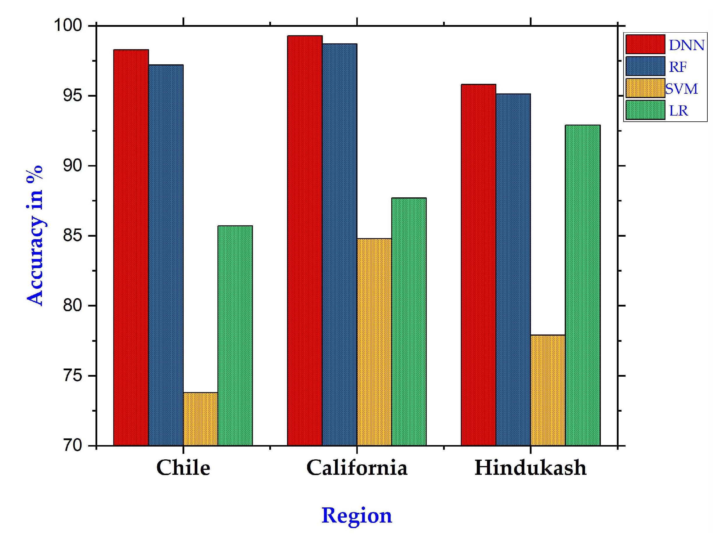
In this research, a trans-disciplinary investigation was carried out, for seismic prediction via machine learning technique. Several machine learning algorithms—including deep neural networks, random forest, support vector machine, and linear regressions—were applied to three distinct datasets: Chile, Southern California, and Hindukush. The algorithms were evaluated on the mentioned datasets, using in-sample and out-of-sample techniques. Our proposed deep neural network approach outperformed the benchmark techniques on all the datasets. On average, the accuracy of the proposed model was 10% better than the benchmark algorithms, while in terms of precision, recall, and F1-score, the performance improvement was 20%, 29%, and 36%, respectively. The same performance order was observed using out-of-sample testing.

Although our model outperformed the existing works, and achieved significantly better performance, it is important to mention that we focused on seismic activity prediction only (classification problem), and did not consider the problem of predicting exact magnitude (regression problem). Furthermore, we did not collect our own data: instead, we used the currently available and already peer-reviewed data. Like all machine learning works, the current work was heavily dependent on the underlying data. Although we have shown that our proposed model was able to achieve better performance than the current techniques, the model may require further testing on other datasets, to strengthen its case. Finally, like all machine learning techniques, our proposed model also suffers from the inherit risk of interpretability.

The proposed technique enriches the body of literature, by proposing a deep-learning-based generalizable architecture for seismic activity prediction. The study should be of interest to trans-disciplinary researchers and practitioners in the domain of seismology. This work could be extended further, by identifying the important features that affected the seismic outcome. Another interesting direction would be to design explainable AI-based techniques.

References

1. World Health Organization. Eartquake Report; WHO: Geneva, Switzerland, 2021. [Google Scholar]
2. Yang, J.; He, F.; Li, Z.; Zhang, Y. An Earthquake Early Warning Method Based on Bayesian Inference. Appl. Sci. 2022, 12, 12849. [Google Scholar] [CrossRef]
3. Ganguly, K.K.; Nahar, N.; Hossain, B.M. A machine learning-based prediction and analysis of flood affected households: A case study of floods in Bangladesh. Int. J. Disaster Risk Reduct. 2019, 34, 283–294. [Google Scholar] [CrossRef]
4. Ahmad, I.; Hamid, M.; Yousaf, S.; Shah, S.T.; Ahmad, M.O. Optimizing pretrained convolutional neural networks for tomato leaf disease detection. Complexity 2020, 2020. [Google Scholar] [CrossRef]
5. Oktarina, R.; Bahagia, N.; Diawati, L.; Pribadi, K.S. Artificial neural network for predicting earthquake casualties and damages in Indonesia. IOP Conf. Ser. Earth Environ. Sci. 2020, 426, 012156. [Google Scholar] [CrossRef]
6. Jena, R.; Pradhan, B.; Beydoun, G.; Alamri, A.M.; Ardiansyah, A.; Nizamuddin, N.; Sofyan, H. Earthquake hazard and risk assessment using machine learning approaches at Palu, Indonesia. Sci. Total. Environ. 2020, 749, 141582. [Google Scholar] [CrossRef] [PubMed]
7. Ma, Z.; Mei, G.; Piccialli, F. Machine learning for landslides prevention: A survey. Neural Comput. Appl. 2021, 33, 10881–10907. [Google Scholar] [CrossRef]
8. Ahmad, I.; Alqarni, M.A.; Almazroi, A.A.; Tariq, A. Experimental evaluation of clickbait detection using machine learning models. Intell. Autom. Soft Comput. 2020, 26, 1335–1344. [Google Scholar] [CrossRef]
9. Asim, K.M.; Idris, A.; Iqbal, T.; Martínez-Álvarez, F. Earthquake prediction model using support vector regressor and hybrid neural networks. PLoS ONE 2018, 13, e0199004. [Google Scholar] [CrossRef] [Green Version]
10. Izquierdo-Horna, L.; Zevallos, J.; Yepez, Y. An integrated approach to seismic risk assessment using random forest and hierarchical analysis: Pisco, Peru. Heliyon 2022, 8, e10926. [Google Scholar] [CrossRef]
11. Asim, K.M.; Idris, A.; Iqbal, T.; Martínez-Álvarez, F. Seismic indicators based earthquake predictor system using Genetic Programming and AdaBoost classification. Soil Dyn. Earthq. Eng. 2018, 111, 1–7. [Google Scholar] [CrossRef]
12. Majhi, S.K.; Hossain, S.S.; Padhi, T. MFOFLANN: Moth flame optimized functional link artificial neural network for prediction of earthquake magnitude. Evol. Syst. 2020, 11, 45–63. [Google Scholar] [CrossRef]
13. Zhang, L.; Si, L.; Yang, H.; Hu, Y.; Qiu, J. Precursory pattern based feature extraction techniques for earthquake prediction. IEEE Access 2019, 7, 30991–31001. [Google Scholar] [CrossRef]
14. Aslam, B.; Zafar, A.; Khalil, U.; Azam, U. Seismic activity prediction of the northern part of Pakistan from novel machine learning technique. J. Seismol. 2021, 25, 639–652. [Google Scholar] [CrossRef]
15. Al Banna, H.; Ghosh, T.; Taher, K.A.; Kaiser, M.S.; Mahmud, M. An earthquake prediction system for Bangladesh using deep long short-term memory architecture. In Intelligent Systems; Springer: Singapore, 2021; pp. 465–476. [Google Scholar]
16. Mousavi, S.M.; Sheng, Y.; Zhu, W.; Beroza, G.C. Stanford Earthquake Dataset (STEAD): A global data set of seismic signals for AI. IEEE Access 2019, 7, 179464–179476. [Google Scholar] [CrossRef]
17. Dostál, O.; Procházka, A.; Vyšata, O.; Ťupa, O.; Cejnar, P.; Vališ, M. Recognition of motion patterns using accelerometers for ataxic gait assessment. Neural Comput. Appl. 2021, 33, 2207–2215. [Google Scholar] [CrossRef]
18. Prochazka, A.; Vysata, O.; Marik, V. Integrating the role of computational intelligence and digital signal processing in education: Emerging technologies and mathematical tools. IEEE Signal Process. Mag. 2021, 38, 154–162. [Google Scholar] [CrossRef]
19. Panakkat, A.; Adeli, H. Neural network models for earthquake magnitude prediction using multiple seismicity indicators. Int. J. Neural Syst. 2007, 17, 13–33. [Google Scholar] [CrossRef]
20. Reyes, J.; Morales-Esteban, A.; Martínez-Álvarez, F. Neural networks to predict earthquakes in Chile. Appl. Soft Comput. 2013, 13, 1314–1328. [Google Scholar] [CrossRef]
21. Wiemer, S.; Wyss, M. Minimum magnitude of completeness in earthquake catalogs: Examples from Alaska, the western United States, and Japan. Bull. Seismol. Soc. Am. 2000, 90, 859–869. [Google Scholar] [CrossRef]
22. Gutenberg, B.; Richter, C.F. Frequency of earthquakes in California. Bull. Seismol. Soc. Am. 1944, 34, 185–188. [Google Scholar] [CrossRef]
23. Aki, K. Maximum likelihood estimate of b in the formula logN= a-bM and its confidence limits. Bull. Earthq. Res. Inst. Univ. Tokyo 1965, 43, 237–239. [Google Scholar]
24. Shi, Y.; Bolt, B.A. The standard error of the magnitude-frequency b value. Bull. Seismol. Soc. Am. 1982, 72, 1677–1687. [Google Scholar] [CrossRef]
25. Matthews, M.V.; Reasenberg, P.A. Statistical methods for investigating quiescence and other temporal seismicity patterns. Pure Appl. Geophys. 1988, 126, 357–372. [Google Scholar] [CrossRef]
26. Habermann, R. Precursory seismic quiescence: Past, present, and future. Pure Appl. Geophys. 1988, 126, 279–318. [Google Scholar] [CrossRef]
27. Last, M.; Rabinowitz, N.; Leonard, G. Predicting the maximum earthquake magnitude from seismic data in Israel and its neighboring countries. PLoS ONE 2016, 11, e0146101. [Google Scholar] [CrossRef] [PubMed] [Green Version]
28. Khan, A.; Zubair, S.; Al Sabri, M. An Improved Pre-processing Machine Learning Approach for Cross-Sectional MR Imaging of Demented Older Adults. In Proceedings of the 2019 First International Conference of Intelligent Computing and Engineering (ICOICE), Hadhramout, Yemen, 15–16 December 2019; pp. 1–7. [Google Scholar]
29. Ying, X. An overview of overfitting and its solutions. J. Phys. Conf. Ser. 2019, 1168, 022022. [Google Scholar] [CrossRef]
30. Mannor, S.; Peleg, D.; Rubinstein, R. The Cross Entropy Method for Classification; Association for Computing Machinery: New York, NY, USA, 2005; pp. 561–568. [Google Scholar] [CrossRef] [Green Version]
31. Wright, R.E. Logistic regression. In Reading and Understanding Multivariate Statistics; American Psychological Association: Washington, DC, USA, 1995. [Google Scholar]
32. Kecman, V. Support vector machines—An introduction. In Support Vector Machines: Theory and Applications; Springer: Berlin/Heidelberg, Germany, 2005; pp. 1–47. [Google Scholar]
33. Svetnik, V.; Liaw, A.; Tong, C.; Culberson, J.C.; Sheridan, R.P.; Feuston, B.P. Random forest: A classification and regression tool for compound classification and QSAR modeling. J. Chem. Inf. Comput. Sci. 2003, 43, 1947–1958. [Google Scholar] [CrossRef] [PubMed]
34. Hossin, M.; Sulaiman, M.N. A review on evaluation metrics for data classification evaluations. Int. J. Data Min. Knowl. Manag. Process 2015, 5, 1. [Google Scholar]
Figure 1. Research workflow.
Applsci 13 01598 g001
Figure 2. The Proposed Deep Neural Network Architecture.
Applsci 13 01598 g002
Figure 3. Overall accuracy score of all approaches on each dataset.
Applsci 13 01598 g003