Article

ATICVis: A Visual Analytics System for Asymmetric Transformer Models Interpretation and Comparison

Department of Computer Science and Information Engineering, National Taiwan Normal University, Taipei 116, Taiwan
*
Author to whom correspondence should be addressed.
Appl. Sci. 2023, 13(3), 1595; https://doi.org/10.3390/app13031595
Submission received: 29 December 2022 / Revised: 14 January 2023 / Accepted: 15 January 2023 / Published: 26 January 2023
(This article belongs to the Special Issue Explainable AI (XAI) for Information Processing)

Abstract

:
In recent years, natural language processing (NLP) technology has made great progress. Models based on transformers have performed well in various natural language processing problems. However, a natural language task can be carried out by multiple different models with slightly different architectures, such as different numbers of layers and attention heads. In addition to quantitative indicators such as the basis for selecting models, many users also consider the language understanding ability of the model and the computing resources it requires. However, comparing and deeply analyzing two transformer-based models with different numbers of layers and attention heads are not easy because it lacks the inherent one-to-one match between models, so comparing models with different architectures is a crucial and challenging task when users train, select, or improve models for their NLP tasks. In this paper, we develop a visual analysis system to help machine learning experts deeply interpret and compare the pros and cons of asymmetric transformer-based models when the models are applied to a user’s target NLP task. We propose metrics to evaluate the similarity between layers or attention heads to help users to identify valuable layers and attention head combinations to compare. Our visual tool provides an interactive overview-to-detail framework for users to explore when and why models behave differently. In the use cases, users use our visual tool to find out and explain why a large model does not significantly outperform a small model and understand the linguistic features captured by layers and attention heads. The use cases and user feedback show that our tool can help people gain insight and facilitate model comparison tasks.

1. Introduction

Natural Language Processing (NLP) is one of the important applications of artificial intelligence. With the gradual maturity of AI technology in recent years, the market scale of NLP applications in the industry is also expanding. For example, American Airlines’ Twitter messages are used for sentiment analysis. Customers’ sentiments are classified as positive, neutral, and negative to infer customers’ satisfaction. Because NLP applications have increased in importance, more and more scientists are devoted to NLP research, and many deep learning architectures have been developed to deal with natural language problems. Transformer [1] is one of the most popular architectures for NLP applications in recent years. Its emergence allows machine learning experts to introduce a larger and more powerful model because Transformer solves the problem that sequential neural networks cannot be trained effectively by performing parallel operations. Transformer has gained great success and attention since it was proposed and multiple natural language processing learning techniques have been developed based on Transformer, such as BERT [2], XLNet [3], GPT [4] and GPT-2 [5]. These models also have been successfully applied in various NLP applications, which include translation in various languages, sentiment analysis and even image classification [6].
One NLP task can often be accomplished by multiple different models. These models could be developed based on different Transformer architectures, such as BERT or XLNet [3], or the same Transformer architecture with different parameter configurations, such as different number of layers. Comparing models is a crucial task when users train, select or improve a model for their NLP tasks. For example, a model trainer may want to know whether an advanced and larger model is a better choice because it may be overkill for a task and requires a longer prediction time and memory space. Model users may want to explore error patterns between models with similar prediction accuracy to select one that better fits their tasks. Understanding the similarity and differences of models’ decision-making processes could inspire architects to propose advanced architectures. Although many quantitative metrics, such as F1 score, AUC or TF-IDF etc., have been used to understand the performance of models, these classic quantitative metrics may not be sufficient if users want to know the reasons of why models behave differently in detail to select a proper model or redesign a new model.
To “open the black box” and deeply understand the deep learning models, many visual analytics tools have been proposed to help machine learning experts. RNNVis [7], CNERVis [8] and M2lens [9] have been proposed to interpret and debug RNN, LSTM and multimodal models for NLP applications, respectively. Although these visual tools are developed to interpret deep learning models with sequential inputs, these works do not focus on the complex transformer-based model interpretation and comparison. Derose et al. [10] proposed a visual analytics tool to explore the differences of attention flows between pre-train and fine-tuning of a transformer-based model. However, the tool can only compare the transformer-based models with the same architecture instead of asymmetric architectures. Several visual analytics tools [11,12,13] have also been proposed to compare different deep learning models. However, most of these works focus on the deep learning models for images, medical and other applications and are hard to port to NLP applications.
To facilitate the comparison of transformer-based models with architecture variants, we propose a visual analytics tool (Figure 1) that allows users to interactively explore the models’ decision-making processes in detail and gain insight into the reasons for the performance differences. Our tool guides users to compare asymmetric models from the model, layer, attention head, to attention word levels. We summarize the information from models in different aspects, such as instance labels, classification results, prediction confidences, and possible captured linguistic features for users to explore the difference between models. One of the challenges of comparing asymmetric transformer-based models is identifying critical layers from many possible layer combinations. Our system evaluates the similarity between layers by comparing what the classification tokens of two layers pay attention to in the same instance. We summarize and visualize the similarity between layers for users to identify interesting layer combinations for further exploration. The same strategy is also used to show the similarity among attention heads. Instance level comparison overview is also provided for users to identify and select critical instances to analyze the difference between models deeply. The word information encoded by attention vectors of heads is summarized and shown for the comparison of the head-to-head relationship and linguistic knowledge learned by models. We demonstrate our system by use cases to show that our system can assist users in efficiently interpreting the roles of layers and heads of different models, explain why a much more complex model does not provide significant performance improvement, and identify the layers and heads that extract duplicated information to suggest the direction for the model improvement. After domain experts use our system, domain experts also comment on our visual tool. The feedback and suggestions from domain experts are also summarized at the end of this paper.
In summary, the contributions of this study are the following:
  • We propose metrics to evaluate the captured information similarity between layers and attention heads. This helps users to identify layer and head combinations worth to compare and reduces the complexity when users compare models.
  • A complete and convenient interactive visualization system is developed for experts to interpret and compare transformer-based models easily.
  • Use cases are shown to demonstrate how the proposed system helps NLP experts understand their models and make decisions. In addition, user feedback is collected to discuss the pros and cons of our current system.

2. Related Works

2.1. Language Model

Language model is an important natural language processing technology, representing the syntactic and semantic properties captured in the words or sentences. Bengio et al. [14] first proposed the concept of word vector. Collobert et al. [15] used the word vector method as an effective tool for downstream task processes, and they also introduced the neural network model structure, which builds the foundation for the improvement of many current NLP techniques. The word vector technique becomes popular after Word2vec technique is proposed by Mikolov et al. [16]. After Pennington et al. released GloVe [17], word vector methods become mainstream in the NLP field. In the past decade, deep learning techniques become the most popular approaches for NLP tasks. Recurrent neural networks (RNNs) [18] is the first deep learning approach widely used. Then, variants of RNN, such as Long Short Term Memory (LSTM) [19] or Gated Recurrent Units (GRUs) [20], also become popular and are used to solve different NLP challenges. In recent years, the transformer [1] architecture has gradually replaced recurrent models because of its efficient training speed by parallel operations and high accuracy. BERT [2] is one of the famous transformer-based deep learning models. Usually, a pre-trained model is trained from a large-scale training dataset and a huge amount of computational resources by large organizations. Users can fine-tune pre-trained Transformer models for their own supervised NLP tasks, e.g., sentiment analysis [21], named entity recognition [22] or text generation [23], with relatively less computational power.

2.2. Model Interpretation

In recent years, language model interpretation has attracted more and more attention because opening the black box of the model can help machine learning experts to understand, diagnose, and improve models. Overall, the model interpretation research works can be categorized into three main classes: model understanding, debugging, and refinement [24,25,26]. Liu et al. [27] designed a visualization system for convolutional neural networks that can help experts understand and diagnose deep convolution neural networks. Ming et al. [7] designed a visual tool to analyze the sentence-level behavior of RNNs sequentially. Strobelt et al. [28] created a visual tool to help users investigate causal effects when changing parts of the model. Tenney et al. [29] proposed a framework to parse the parts of speech, entity recognition, and various dependencies captured by different layers in a pre-training model. Hao et al. [30] illustrated the low-level layers’ and high-level layers’ losses during fine-tuning. These studies gain success in terms of model interpretation. Recent visual analysis works of language models have gradually shifted their focus to the transformer-based model [31,32]. These works can help users understand a model’s behaviors deeply, but these systems do not support model comparison.

2.3. Model Comparison

When comparing the models, users often rely on quantitative metrics, such as accuracy, F1-score, mean-square error etc. There are many visualization libraries for model comparison built on top of these metrics. For example, WIT [33], Tensorflow [34], Scikit-learn [35]. However, when users want to retrieve more information, such as comparing decision-making processes of models, these metrics do not provide sufficient details and users are usually more interested in the underlying details. Therefore, many visual analytics comparison tools are proposed for users to interactively acquire the underlying details for model comparison. Ming et al. [7] developed RNNVis for users to explore and compare the hidden behavior of different models. Piringer et al. [36] proposed an interactive approach called HyperMoVal that is designed to support multiple tasks related to model validation. Muruges et al. [37] designed a visual system that enables users to systematically and deeply explore the differences from two models. Wang et al. [38] introduced multiple metrics to identify meta-features with the most complementary behaviors of two classifiers. Apart from the linguistic relationship, Matthew Berger’s research [10] points out that models can capture not only linguistic dependencies but also their meaning. Although these visual analytics systems are developed to compare multiple deep learning models, extending these systems to compare asymmetric and complex transformer-based deep learning models is not trivial.

3. Backgrounds

In this section, we will introduce the fundamental knowledge of transformers. In many transformer architecture models, a special classification token [CLS] is often added to the input sentence. For classification tasks, the first token (corresponding to [CLS]) is used as the “sentence vector”. [CLS] token itself does not represent any specific meaning, so [CLS] token is considered to represent the meaning of the whole sentence more fairly in the process of learning. This paper uses the attention vector of the [CLS] token as a basis to build the visual analytics tool. The attention mechanism [20] is proposed to improve the performance of recurrent models, such as LSTM and GRU. Attention mechanism is also widely used in many fields such as machine translation [39], entailment reasoning [40] and image caption [41]. At the same time, Attention itself can be used to explain the alignment relationship between translation input/output sentences, explain what the model has learned, and open the black box of deep learning for users. Self-attention [1] is very different from traditional attention mechanisms. The traditional attention is calculated based on the hidden state of the encoder and decoder. The attention represents the dependency between each word from the decoder to the encoder. However, self-attention captures the dependencies between its own words and words in the encoder and decoder respectively. Self-attention solves the problem of information loss caused by RNN in long texts. Transformer is a network architecture based on self-attention. The transformer models have shown success in many natural language processing tasks. Recently, many models have used transformers as their foundations, and their applications can even be extended to images [42].
Before discussing the tasks we aim to support, we first discuss the extracted representations used in this work. When a text is an input into the model, an attention vector is generated for each word corresponding to each layer in the model (Figure 2). In this paper, we use the attention vector of the [CLS] token to examine the linguistic information captured by the model. The values in the attention vector correspond to the input words, respectively, and the language information that the model captures is checked by the attention values corresponding to the words (Figure 3).
In addition, the transformer architecture has multiple heads, forming multiple subspaces and allowing the model to capture different information. We introduce the calculation of an attention vector from multiple attention heads. When considering a layer l, a sequence of tokens s = ( w 1 , w 2 , , w n ) , X l = [ x 1 l , x 2 l , x n l ] is embedding vectors of n inputs words from layer l. The dimension of embedding vector of each word is d, so X R n × d . The representation of vectors Q, K, V are obtained through the linear transformation of W q , W k , W v R d × d . W q , W k and W v are projection matrices from a d-dimensional space to a d -dimensional space and we can calculate Q l , K l and V l by Q l = X l W q , K l = X l W k , V l = X l W v . Attention matrix is A l R n × n and calculated based on Q and K, and d k as a scaling factor. i is the index of the head. The Equation (1) is the calculation of the attention matrix for one layer and we show an example of the attention computation in Figure 4.
A i l ( Q i l , K i l ) = s o f t m a x ( Q i l ( K i l ) T d k )

4. Goals and Requirements

Figure 5 shows the steps to develop our system. We first must understand users’ needs and perform the requirement analysis to design the prototype. After implementing the system prototype, users will use the system and give feedback again. Based on the feedback, we will redesign and improve the system. After the system design procedure and system development, we summarize the final goal and design requirements that need to be accomplished to serve user analysis purposes in this section.

4.1. Design Goals

G1: Connect the roles of layers and attention heads to linguistic meaning. In transformer-based models, each attention head of a layer could implicitly represent some linguistic features. Multi-head of a layer are combined into one attention vector that represents the linguistic extracted from the layer. By knowing the linguistic meaning captured by attention heads and layers, users can not only judge whether a model learns rational linguistic features but also can develop prior knowledge to facilitate model behavior comparison tasks.
G2: Understand the decision-making process of instances through self-attention. Examining the decision-making process of interesting instances can often help users to deeply understand the behavior of models. Because self-attention is one of the most important components of the transformer-based model and the attention words are easy to connect to linguistic meaning, summarizing and visualizing the attention information can help users to gain intuition about how the model interprets the instances. By knowing the decision-making process, users can know whether the model carried out a rational task for the classification and build confidence in a model.
G3: Explore potential sources that result in the performance differences. One of the major model comparison purposes is to find out what factors affect the model’s overall classification performance. For example, users may want to know why two similar architectures have quite different classification accuracy, or why a much more complex model does not improve accuracy significantly. When users know this information, users can consider the pros and cons of models to select a model for their tasks better.

4.2. Design Requirements

According to our goals, we propose the following design requirements.
R1: Provide quantitative information about models. Before deeply exploring the models, observing models’ basic quantitative information, such as the number of training instances, accuracy, false positive rate etc., allows users to have a preliminary understanding about models.
R2: Summarize and visualize the similarity of layer combinations and head combinations between models. Each layer and attention head can capture different linguistic features. To compare the layers and heads in detail could facilitate the model comparison task. However, figuring out the layer and attention head combinations worth exploring is not an easy task. Therefore, our system should guide users to find the critical layer and attention head combination for further exploration.
R3: Identify similar heads at each layer in a single model. Examining the linguistic behavior of multiple heads costs time. Identifying heads with similar behaviors can save a lot of time when examining the behavior of each head and users can more quickly summarize the role of each layer of the model. Summarizing the behavior of these heads in the model can help and reduce search space when comparing models.
R4: Assist users to find out the crucial instance sets for the model comparison task. Comparing how models extract features from the same instances can help users deeply understand the difference between models. For example, instances that two models disagree with each other or instances with completely different attention words from two models. Our system should provide the overview and interface for users to efficiently identify and select these instance sets.
R5: Track and show the formation of classification token by attention words at the sentence level. The classification token summarizes what a layer of the model learns and the token is used for the final classification. By summarizing how a classification token combines attention information and evolves from low to high layers, users can interpret how the model understands the linguistic meaning of a sentence.
R6: Summarize the token level attributes of attention words. Token-level attributes, such as part-of-speech or named entity etc., are the most fundamental linguistic features. Summarizing and comparing which category of the fundamental linguistic features are mainly focused by an attention head or a layer can better connect what they learn to linguistic meanings.

5. Visualization Design

Our visual analytics tool consists of six views, basic information view, layer similarity view, head similarity view, scatter view, attention view, and attention summary view. In addition, because evaluating the similarity between layers and attention heads is one of our visual design tasks (T2) to guide users to find the interesting layer and head combinations, we will first introduce layer and head similarity evaluation and introduce these views in detail. In this section, we call two models compared by users Model A and Model B.

5.1. Layers and Heads Similarity Evaluation

Because transformer-based models have multiple layers and attention heads, going through all layer and head combinations and comparing the difference in what the layers and heads learn is not practical. Our system should evaluate and summarize the similarity of information learned by layers or heads to guide users to identify interesting layer and head combinations. [CLS] token is used as an aggregated sentence representation [43] so [CLS] token can be considered as the representation of the whole sentence’s semantics. In addition, an attention head vector of the [CLS] token can be interpreted as the sentence information extracted by the attention head. Therefore, we summarize test instances’ attention head vectors of [CLS] token to evaluate the similarity of information extracted from two heads of [CLS] token. We use the cosine distance of two attention head vectors of the same instance to represent the similarity of information extracted from two heads on the same instance, and the similarity of two heads is defined by the average similarities of all instances. Equation (2) is the similarity between two heads.
H e a d S I M i , j = k = 1 N c o s ( T i k , T j k ) N
where i represents an attention head of Model A and j represents an attention head of Model B. H e a d S I M i , j is the similarity between these two heads, T i k and T j k are attention vectors of T k , N is the number of test sentences to evaluate the similarity between these two heads, and c o s ( . ) is the cosine similarity function.
To calculate the similarity between two layers, we compute the average head similarities of all head combinations between the two layers.
L a y e r S I M l , l = i = 0 , j = 0 h , h H e a d S I M i , j H * H
where l is a layer of Model A, l is a layer of Model B, H is the number of heads of model A, and H is the number of heads of model B. L a y e r S I M l , l is the layer similarity between layer l and l , i is the head index of layer l, and j is the head index of layer l .

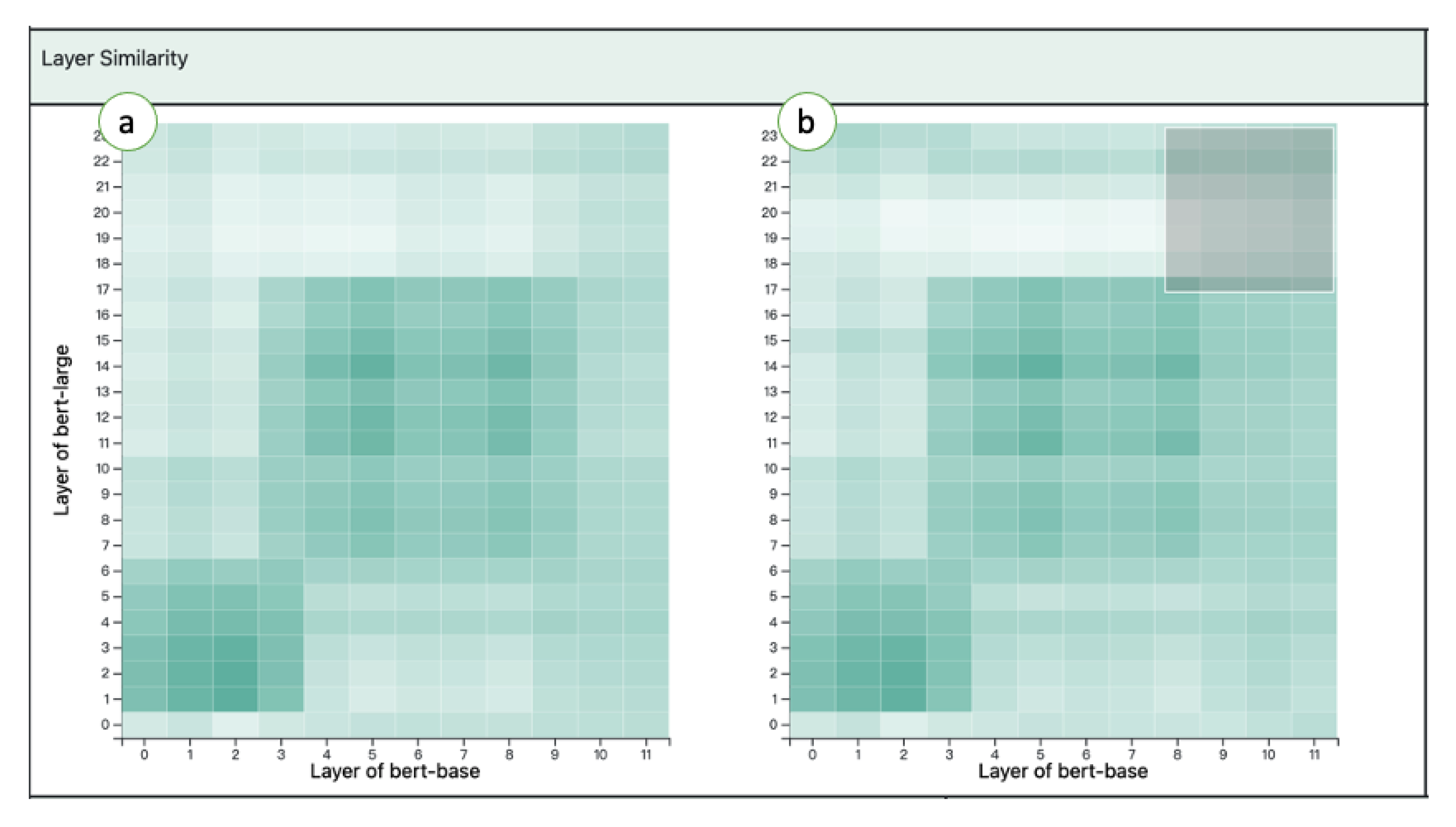
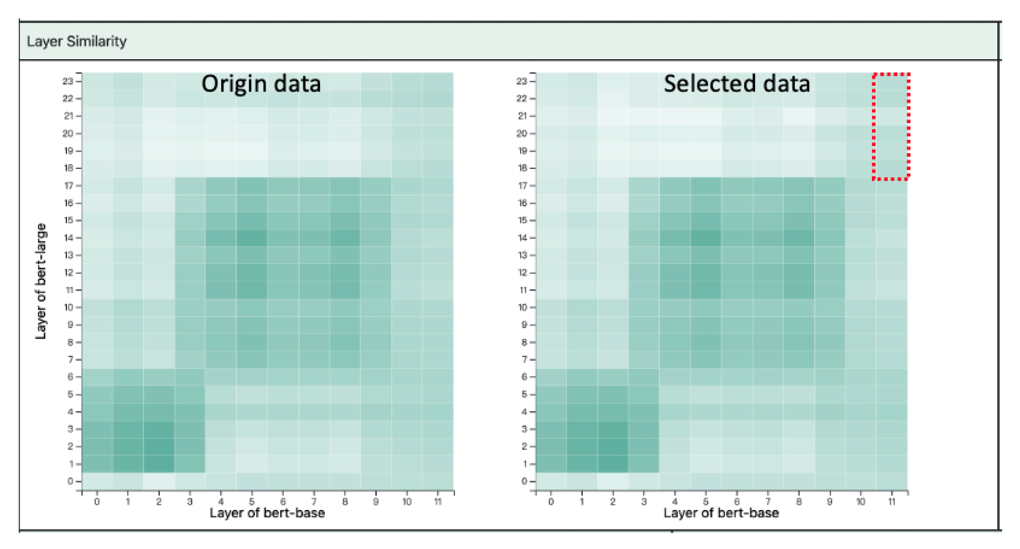
5.2. Layer Similarity Graph

To assist users in identifying interesting layers and comparing them between two transformer-based models (R2), we utilize the Equation (3) to create a layer similarity graph (Figure 6). The main purpose of the layer similarity graph is to provide an overview for users to observe the similarity among layers and identify groups of layers. Because a heat map can provide audiences with obvious relevant visual cues, we use a heatmap to represent the similarity between layers in both models. The horizontal axis and the vertical axis represent layers of two models, and the layers on the two axes are ordered from low to high layers. The saturation of each square encodes the similarity between layers, and a higher saturation color indicates that the two layers are more similar. Figure 6 is an example of the layer similarity graph showing the similarity between transformer-based models with 12 layers and 24 layers. In this example, users can not only identify layer combinations they may be interested in but also observe blocks with high saturation color. Each layer group could focus on relatively similar linguistic features. Users can click on the square when they find a layer combination they are interested in, and a head similarity graph for the combination will be shown. We will introduce the head similarity graph in Section 5.3.

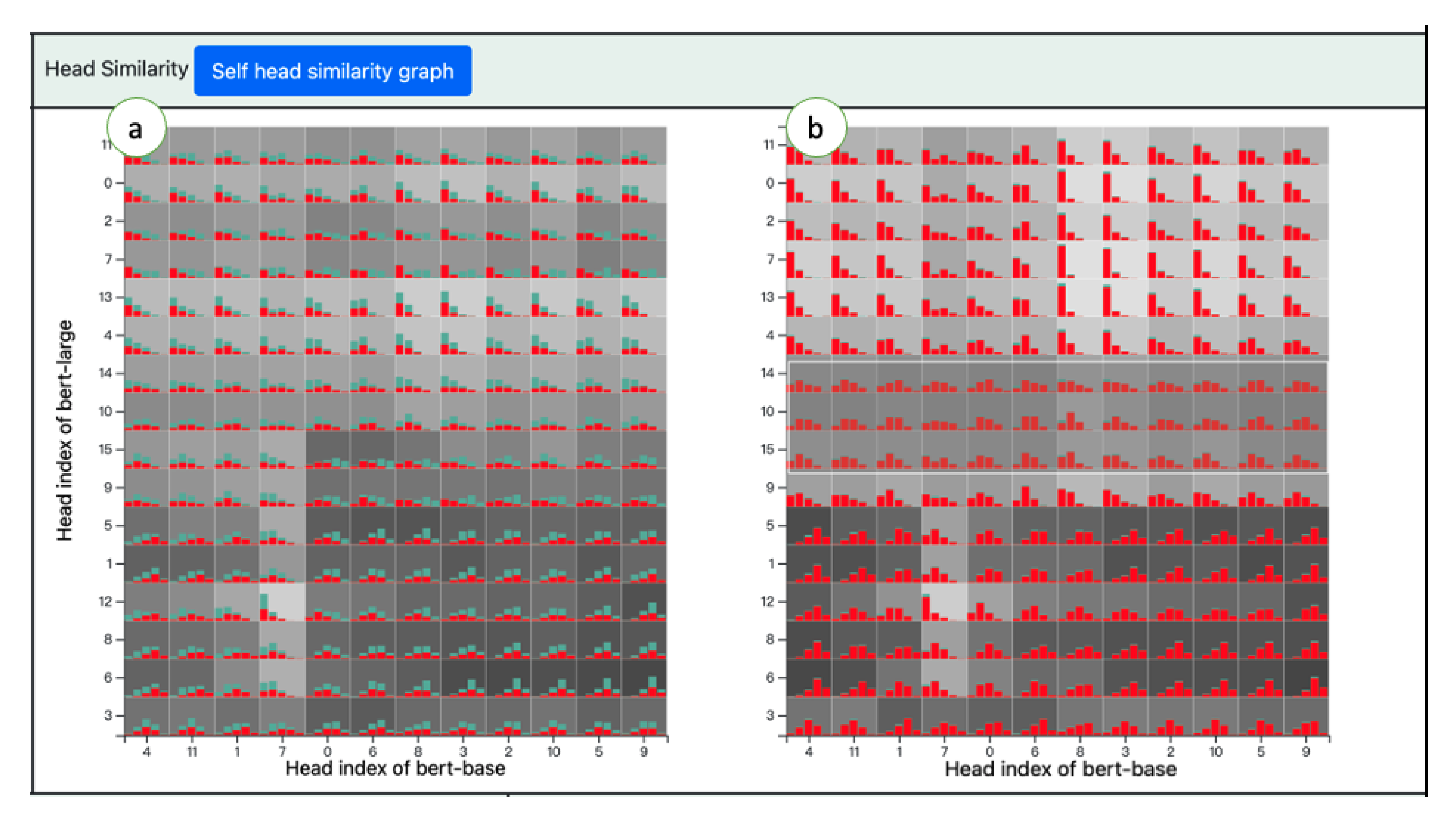
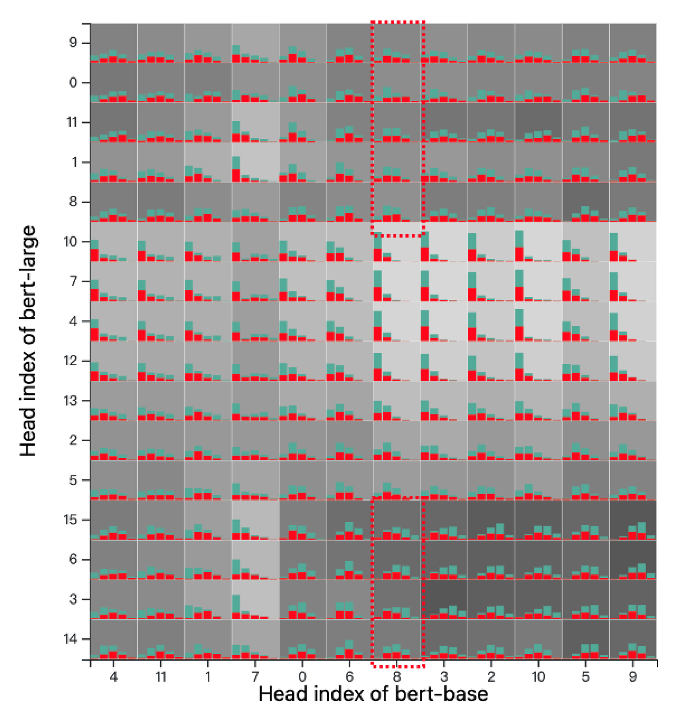
5.3. Head Similarity Graph
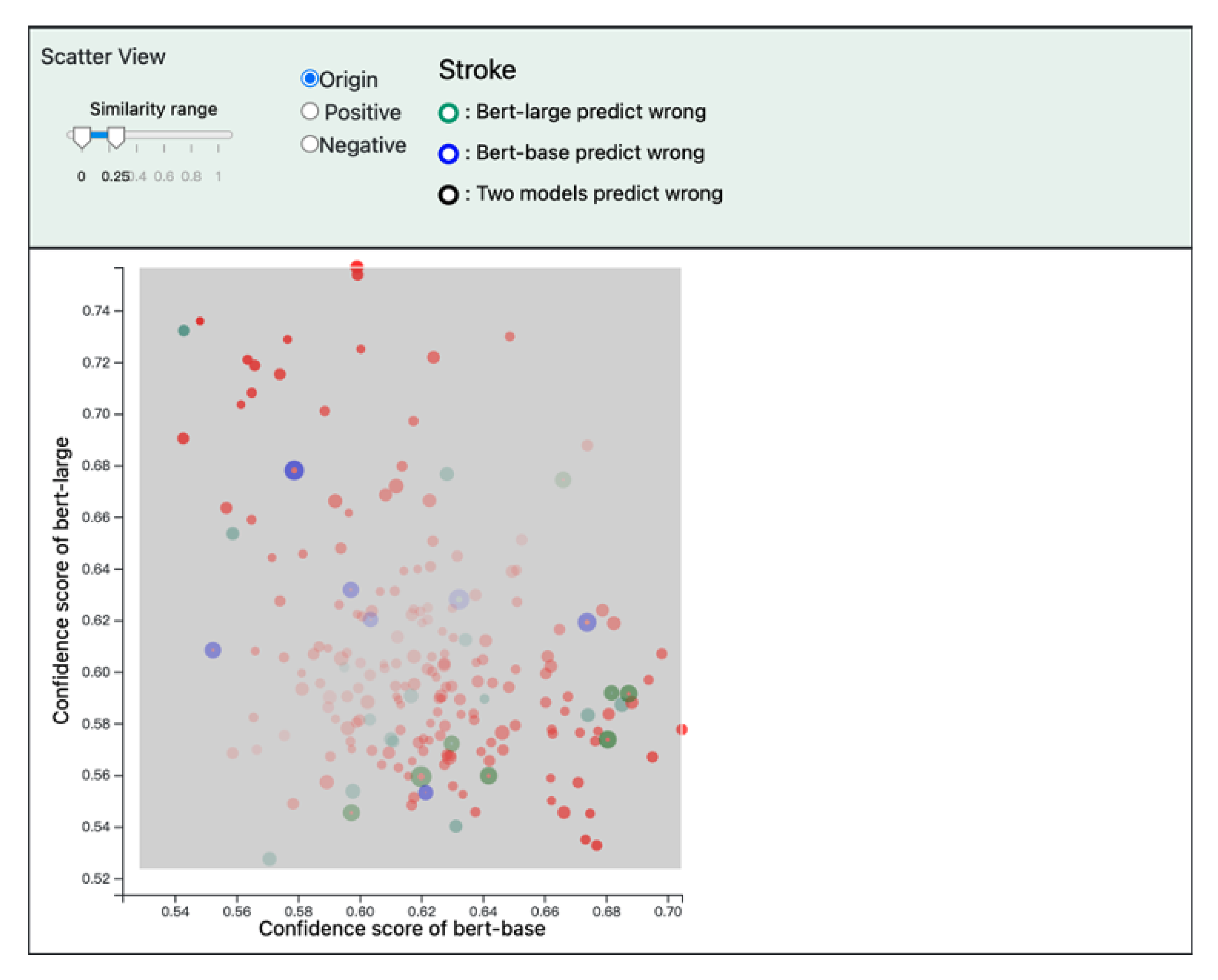
The information captured by a layer of the transformer-based model is combined from multiple attention heads of the layer. Therefore, comparing attention heads between two models can allow clear and deep understanding of the different behaviors of models (R2). However, the number of head combinations between the two selected layers of the two models is usually more than one hundred. Finding the head combinations worth exploring is not an easy task. Therefore, we also develop a head similarity graph similar to the layer similarity graph in Section 5.2. Figure 7 is two similarity graphs and the two axes represent the attention heads of the two layers selected from the layer similarity graph. The saturation color represents the attention head similarity computed by Equation (2). A higher saturation color indicates that the two attention heads are more similar. Although each head of a layer usually has an index, the index does not relate to the order of processing sentences. To help users quickly identify head groups that could extract similar linguistic features, we should put heads that extract similar linguistic features next to each other. A common practice is to use hierarchical clustering [44] to create a dendrogram [45] and order the two axes according to the result of the dendrogram. We use Equation (2) as the distance function when clustering heads of a layer. Figure 7 is the head similarity graph after head reordering. In this example, the 1st, 6th, and 9th heads of the x-axis are close to each other because the linguistic feature extracted from them are similar to each other (Figure 7a). In addition, the dark block at the bottom of Figure 7a shows that the 1st, 6th, and 9th heads of the x-axis and the 3rd, 4th, 6th, 9th, 14th, and 15th heads of the y-axis could extract similar linguistic features. Users sometimes want to compare the similarity among heads of a layer within one model to identify similar heads without interference from the second model (R3). Users can click the button “Self head similarity graph” in Figure 7 to show self head similarity graph of each model (Figure 8). The way to generate the self-head similarity graph is the same as that to generate the head similarity graph.
In addition, summarizing and showing similarity at the instance level helps users find interesting head combinations (R4). Therefore, we add the bar chart to each square in the head similarity graph to show the similarity histogram of each head combination. The similarity of an instance between two heads is calculated by the cosine similarity function in Equation (2). The horizontal axis of each similarity histogram is the similarity value, increasing from left to right on the axis. The vertical axis of each similarity histogram represents instance count, and the bar color indicates the ground truth label of the instances. With the similarity histograms, users could find some head combinations with interesting instance-level patterns. For example, the bars in most squares are uniformly distributed, but a few squares have bars right-skewed. The users are often interested in these head combinations with special distribution (Figure 7b). After users find a head combination they are interested in, they can click on the square of the head combination to compare two models at the instance level in a scatter view (Figure 9). We will introduce the scatter view in Section 5.4.

5.4. Scatter View

When users are interested in a head combination, a scatter view in our system shows instance-level information from the two heads for users to select instances to future compare extracted information from the same instance set (R5). The scatter plot shows the classification confidence scores, confidence score difference between the two models, and instances’ attention vector similarity between two attention heads. Figure 9 is an example of the scatter plot. Each circle in the scatter plot represents an instance. The two axes represent the classification confidence scores of the two models. The color, circle size and opacity encode the labels of instances, the attention vector similarity between two heads, and the confidence score difference respectively. The stroke color of a circle encodes whether models predict an instance correctly. The blue stroke color and green stroke color represent the prediction from one of the models is incorrect. The black stroke color represents both models predict incorrectly. Users can find out some special instances, such as an instance with quite different confidence scores from two models for further exploration.
Our system also provides three interactions for users to select a subset of instances. Users can show instances within a similarity range by dragging the similarity range slider, display instances with the same label by the radio buttons, and select instances by brushing a region. After selecting a subset of instances, our system recalculates the layer similarity graph and the head similarity graph using the selected instances only. These two new graphs calculated are called filtered layer similarity graph and filtered head similarity graph. Our system arranges them next to the original layer similarity graph and head similarity for the side-by-side comparison (Figure 10 and Figure 11). Users can compare and figure out models that have a significantly different behavior when processing the subset of instances.

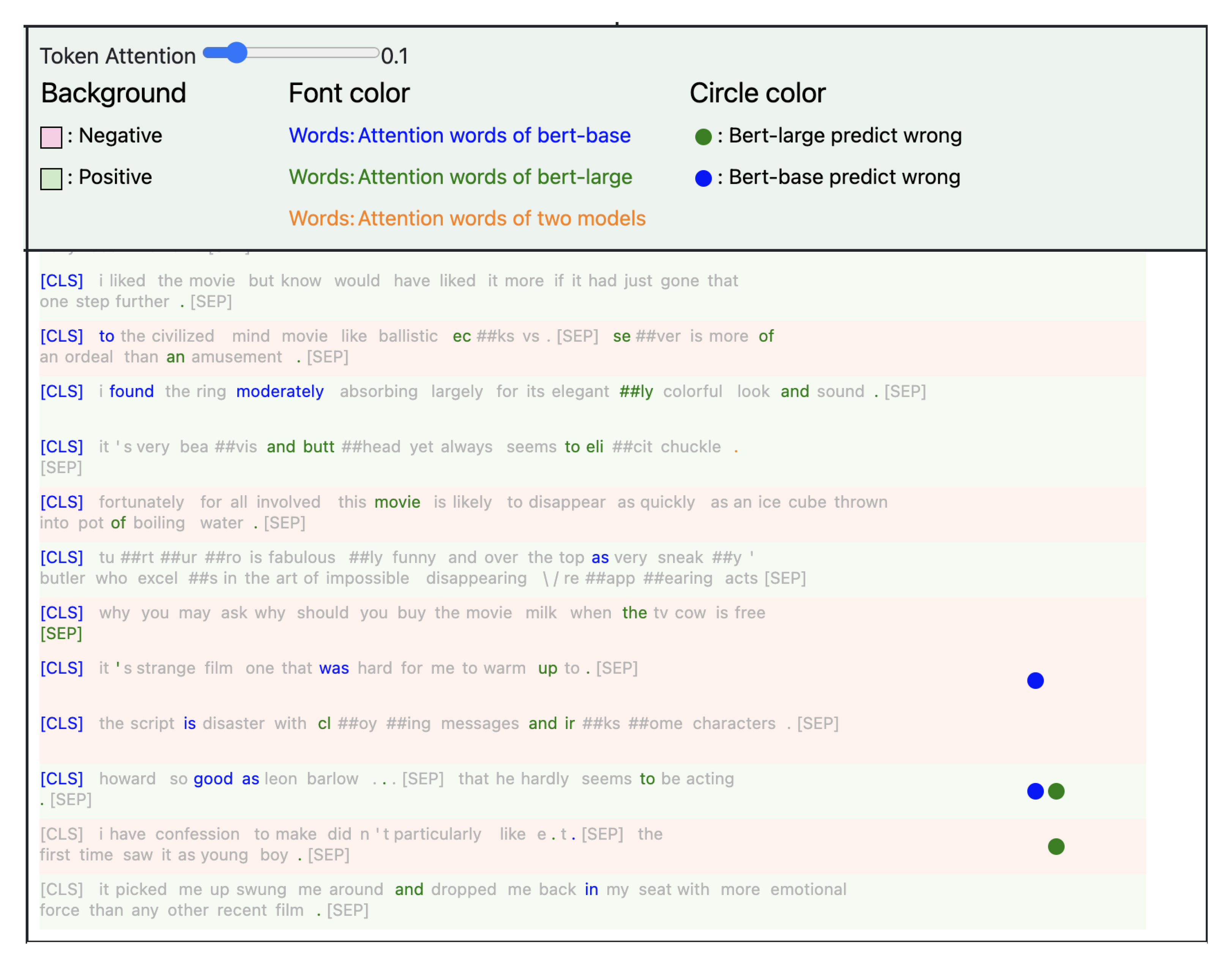
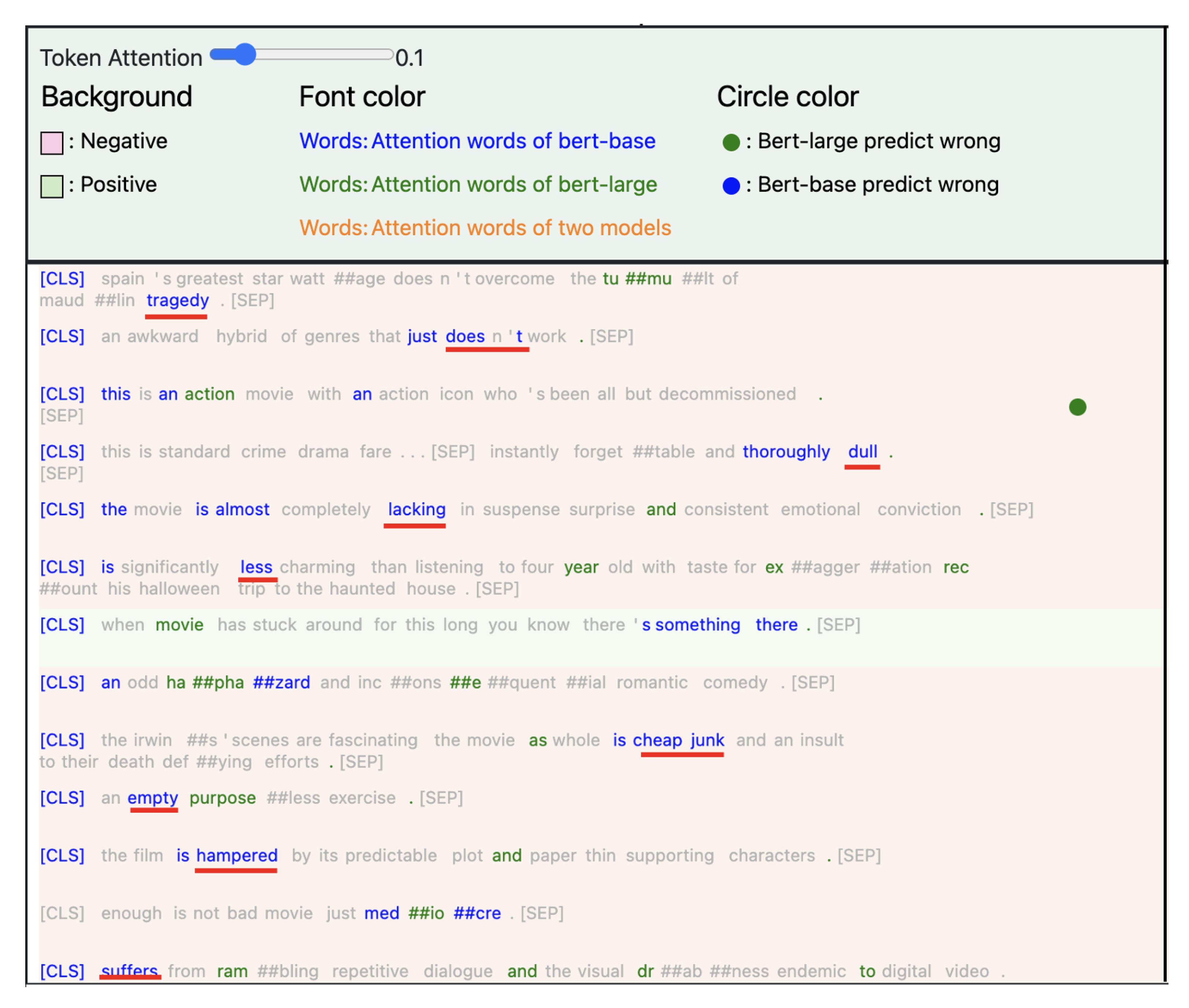
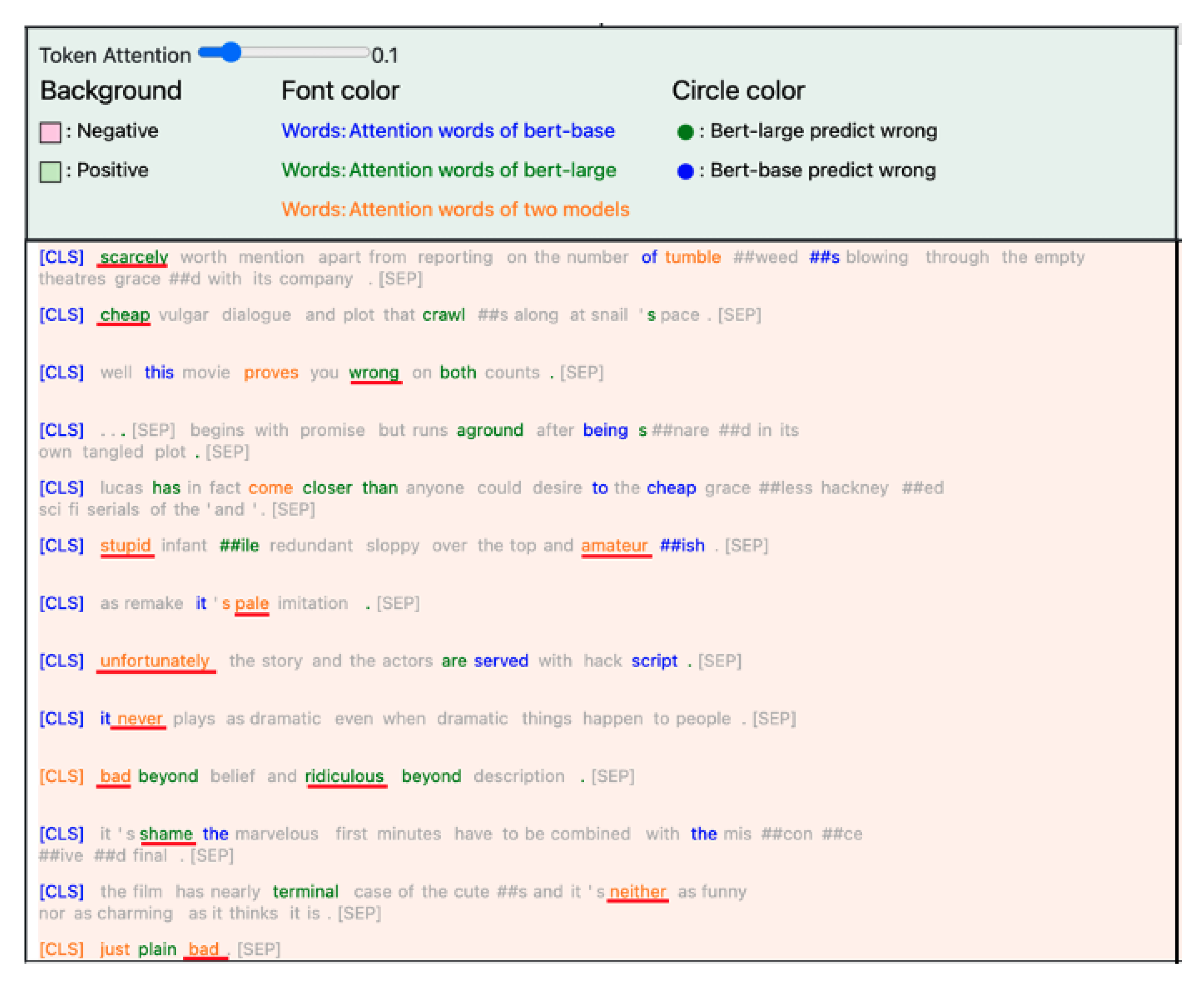
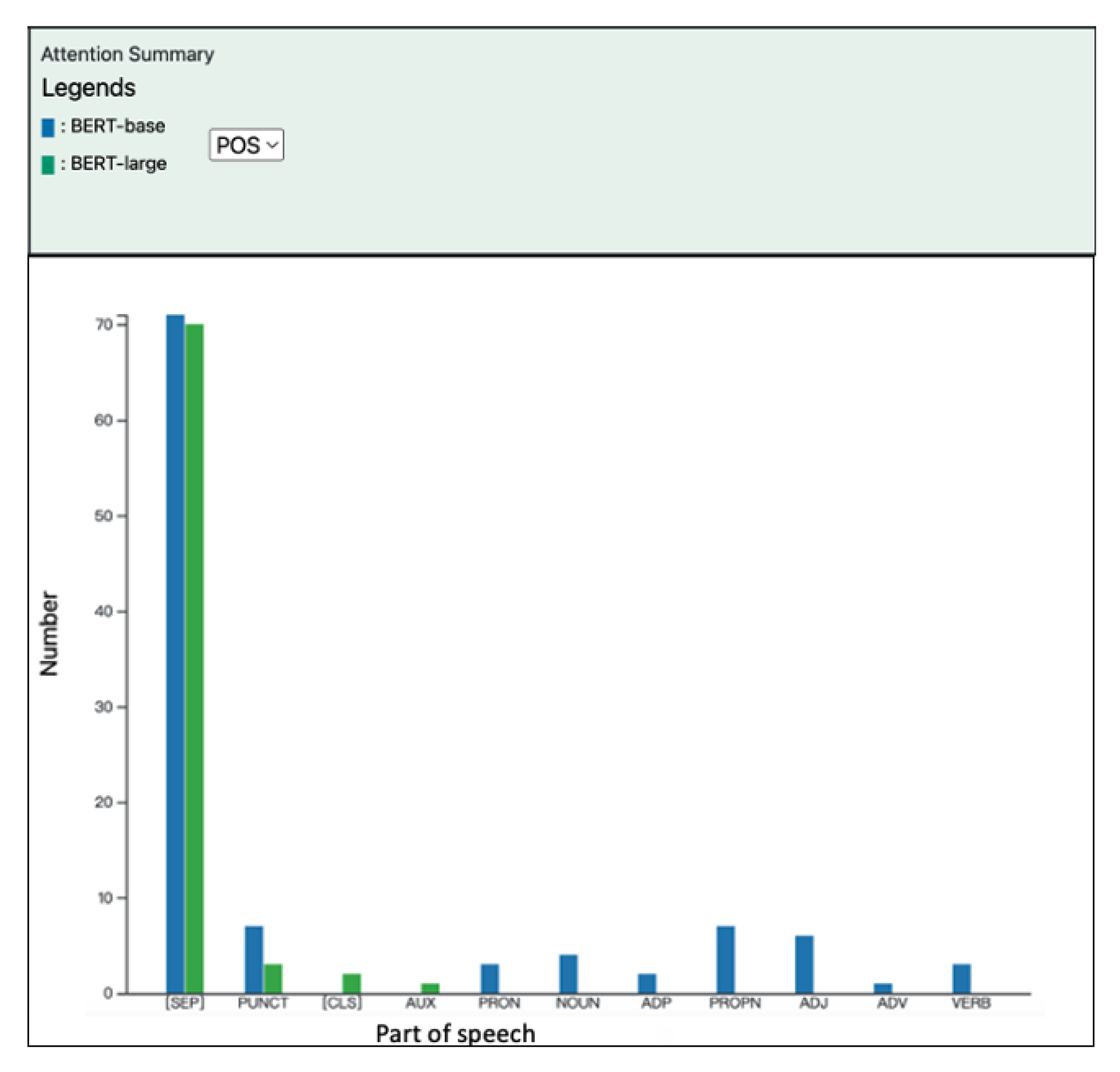
5.5. Attention View and Attention Summary

The attention view (Figure 12) shows the sentences selected in the scatter view and highlights the information focused by the selected heads of two models from the head similarity groups (R5). Because the [CLS] token can represent the information of the whole sentence [10,46] and the attention vector of the [CLS] token indicates the impact of each word when producing the [CLS] token, we define that the attention words are the words whose weights in the attention vector of the [CLS] token are greater than a user-defined threshold. Users can adjust the threshold by the slider at the top of the attention view. The attention view allows users to observe the mutual attention words of two models and summarize the mutual linguistic meaning captured by heads. The word with blue or green color indicates that the word is the attention word of one of the two models. The word with orange color indicates that the word is the attention word of both models. In addition, we also encode the labels of instances and prediction results of both models in the attention view. The background color encodes the labels of instances. Small circles may attach at the right-hand side of an instance. An instance with blue and green small circles indicates that the corresponding models incorrectly classify the instance.
We also statistically summarize the fundamental linguistic attributes of attention words, such as part-of-speech or name entity, for users to more intuitively recognize the possible linguistic meaning captured by heads (R6). We use a grouped bar chart to visualize the summarization of linguistic attributes, and we call the bar chart attention summary (Figure 13). The horizontal axis is the class of fundamental linguistic attributes, the vertical axis represents the count of attention words, and the colors encode models.
In addition, our system also supports the comparison between sets of heads from two models (R5). This function allows users to efficiently summarize the differences in attention words and compare linguistic features of head groups. Users can brush the heads of interest on the filtered head view (Figure 11b). The union set of attention words from the selected heads of a model will be the attention words of the head group of the model. The attention view and attention summary will be updated accordingly by the union sets from the two models when users brush heads of interest on the filtered head view.

5.6. System Implementation

Our visual analytics system consists of a front-end interface and a back-end server. The front-end interface includes the implementation of the views of our visual tool introduced in this section and their interactive functions. The front-end implementation is carried out by Javascript and D3 library. The back-end server includes a program to process test instances and data from transformer-based models and return the information to the front-end interface to display. The data process program is implemented by Python and the Transformer information extraction library from Huggine Face Community. The Transformer information extraction library is used to extract the hidden vectors of each layer and the attention weight of different attention. The communication between the front- and back-end is performed by Flask.

6. Use Cases

In this section, we demonstrate our tool using two BERT models with different architectures and we call them bert-base and bert-large. One of them has 12 layers and 12 heads per layer, and the other one has 24 layers and 16 heads per layer. They are trained to complete the text classification task of IMDB dataset. The dataset has 500 profiles with 269 positive texts and 231 negative texts. Figure 14 illustrates the main functions of our system and the flow to use the proposed visual analytics system. When users explore models using our system, these are possible paths and flow to interpret and compare their models.

6.1. Use Case 1: Exploring and Comparing Behaviors of a Large and a Small Models (Video S1)

The user is curious why the bert-large model with more layers and attention heads does not provide a significant accuracy improvement than the bert-base model (Figure 1A). Therefore, the user would like to explore and compare the internal behaviors of the models using our system. First, the user checks Figure 15 (left) and observes that dark green squares distribute around the diagonal of the layer similarity graph. This pattern summarizes that the extracted information from lower to higher layers between two models has a match when classifying instances. In addition, the user also observes that the layer similarity graph shows three darker green blocks around the diagonal. It hints that the layers within the same darker green block may extract similar information. To explore why the large model does not provide significant prediction accuracy improvement, the user decides to compare the subtle difference between layer combinations. Therefore, the user repeatedly clicks on the squares with darker green color and observes the corresponding head similarity graph. When the user clicks on the combination of the last layers of both models, a pattern in the corresponding head similarity graph (Figure 15 (right)) attracts the user’s attention. The user finds that red bar charts of many attention head combinations are left-skewed, indicating that the attention words of negative emotion instances from the two attention heads have a low similarity. The user decides to explore more details. Then, the user clicks the square of the bert-base head index 8 and the bert-large head index 7 on the head similarity graph (orange bar in Figure 13), because this is one of the head combinations with a left-skewed red bar chart.
By observing the values of the x- and y-axes of the scatter view (Figure 16), the user finds that the maximum confidence score of the bert-large model is larger than that of the bert-base model, and the minimum confidence score of the bert-lage model is smaller than that of the bert-base model. Since the user is now interested in instances with low similarity, the user uses the slider at the top of the scatter view to adjust the similarity value range to 0–0.25 and then selects all instances in the scatter view.
In addition, after observing the attention words of these selected instances in the attention view (Figure 17), the user finds that words with blue font, bert-base model’s attention words, often contain negative words. This observation means that the bert-base model’s attention head extracts information from negative words, and the user thinks the attention head would do a logical task to facilitate the classification task.
In the same attention view (Figure 17), the user observes that wordpieces are in green color, which also means that these wordpieces are from the bert-large model’s attention head. Wordpiece is a unique feature of the transformer-based model, and its purpose is just to separate to input sentences. Paying attention on wordpieces may not extract significant linguistic meaning. Therefore, the user examines the other instance by selecting all instances with a similarity value between 0.25–1 in the scatter view. Then, the user finds that the words in green color still often contain wordpieces in the attention view (Figure 18). This observation confuses users because the bert-large model mainly focuses on wordpieces, but the bert-large model still performs well. Therefore, The user guesses the early layers of bert-large model may extract the information extracted by the 8th head of the 11th layer of bert-base model. Therefore, the user starts to find layers of the bert-large model similar to the 11th layer of the bert-base model and close to the last layer. The user repeatedly selects darker green squares on the column of the 11th layer in the layer similarity graph for exploration (Figure 19). Until the user clicks the square of the 11th layer of the bert-base model and the 20th layer of bert-large model and explores it in detail, the user finds the evidence to verify the user’s hypothesis.
Because the 8th attention head of the 11th layer of the bert-base model mainly focuses on the negative words, the user would like to search an attention head of the bert-large model that matches the head in the bert-base model. The user checks the column of the 8th head of the bert-base in the corresponding head similarity graph (Figure 20) of the selected layer combination and focuses on the dark squares. When clicking on the square of the 11th head of the bert-large model and checking the attention words of negative sentences in the attention view, the user finds that many of the negative words are in orange color, indicating the 8th attention head of the 11th layer of the bert-based model and the 11th head of the 20th layer of the bert-large model focus on similar words (Figure 21). In addition, the user also sees that some negative words are in green font, which indicates that the bert-large attention head captures these words but the bert-base attention head does not. The user concludes that the bert-large model captures the information captured by the bert-based model and the information before the last layer. In addition, the bert-large model captures some words that could facilitate the classification task, but the bert-base may not capture the information. Therefore, the bert-large model can have slightly better performance than the bert-based model. However, the rest of the layer in the bert-large model does not capture sufficient meaningful linguistic features, so the bert-large model does not outperform the bert-base model much.

6.2. Use Case 2: Comparison of Parameterized Linguistic Information (Video S2)

A transformer-based model with more layers and attention heads leads to higher consumption of memory resources. Since the transformer architecture has multiple attention heads, the user is curious whether the attention heads of transformer-based models extract duplicate information, and whether a large model captures more linguistic information or is just overkill on a relatively simple task.
Therefore, the user first tries to find the heads that extract similar information by our tool. The user clicks several darker green squares on the layer similarity graph in Figure 22 (left) and examines the corresponding head similarity graphs. The user finds that many head similarity graphs of selected layer combinations with large dark blocks. This pattern indicates that many attention heads of layers could extract quite similar linguistic information. For example, when the user clicks the square of the bert-base model’s 5th layer and the bert-large model’s 11th layer on the layer similarity graph, the user observes that the corresponding head similarity graph (Figure 22 (right)) shows one bright block and one dark block (Figure 22 (right)(A),(right)(B)) Dark squares indicate all head combinations from the two models extract quite similar information. In addition, two attention heads, the 5th and 14th attention heads, of bert-large model do not intersect with the dark block in Figure 22 (right). The user clicks “Self head similarity graph” button at the top of the head similarity graph to further explore the attention heads similarity within each model. By checking the self-head similarity graphs of two models in Figure 23, the user confirms that almost all of the attention heads of bert-base model’s 5th layer extract quite similar information because almost all squares in Figure 23 (left) are pretty dark. Self head similarity graph of the bert-large model (Figure 23 (right)) shows that most of the attention heads of the bert-large heads, except for the 5th and 14th head, also extract quite similar information. To examine what information is captured by these similar attention heads of the bert-base and bert-large models, the user brushes to select the heads that create the dark block in the head similarity graph (Figure 22 (right)(B)). The attention summary (Figure 24) summarizes the attention words of these selected heads. The user observes that most of the attention words from these attention heads are [SEP] tokens. The user knows that the classification accuracy of the bert-large model is still slightly higher than that of the bert-base model from the basic information panel, the user guesses the 5th and 14th attention heads of the bert-large model may extract extra and much more meaningful linguistic features.
The user then focuses on exploring the 14th attention head of the bert-large model. Because the user mainly focuses on the 14th attention head of the bert-large model now, the user randomly clicks a square on the row of the 14th head of the bert-large model in the head similarity view (Figure 22 (right)) to update the attention view (Figure 25). The user finds that the first words of all instances are always green or orange in the attention view. This means that the 14th heads of bert-large model could extract the positional information from the instances. Then, the user examines the 5th attention head of the bert-large model and the user also randomly clicks a square on the row of the 5th head of the bert-large model in the head similarity view (Figure 22 (right)) to update the attention summary (Figure 26). The user observes that the five longest green bars (bert-large model) are NOUN, ADJ, VERB, PROPN, and ADV. This probably indicates that this attention head tries to catch the parts of speech features in the sentences.
From the exploration by our tool, the user finds another potential reason why the bert-large model has slightly higher classification accuracy. That reason is that a few attention heads of the bert-large capture meaningful linguistic information that does not capture by the bert-base model. In addition, the user also finds that many attention heads capture quite similar information. This discovery suggests that a smaller model with fewer attention heads that requires less memory and has a faster prediction speed could still complete the same NLP task with similar classification accuracy.

7. Conclusions and Future Works

In this work, we develop a visual analytics tool to help model users compare asymmetric transformer-based models. We propose metrics that summarize attention vectors of test instances to evaluate the captured information similarity between layer and head combinations. The metrics help users identify the combinations worth for comparison. A visual analytics tool is developed based on an interactive overview-to-detail framework. Experts can input models and their target test instances into our system to test the performance of models, understand the detailed behavior of two models, and explore the reason that results in the performance difference. Experts can not only pick up the better-fit model for their NLP task but also improve the models after knowing the insight of the models. Users use our tool to explore models and explain why a large model does not significantly outperform a small one. Users also use our tool to interpret what linguistic features each layer and attention head would like to capture. We also interview experts and obtain their feedback. By their feedback, the design of the layer similarity graph can indeed help them quickly understand whether the learning process between models is similar. They agreed that the system’s design process was effective for comparing two models and identifying model details. At the same time, experts in the field also pointed out the weaknesses. The scatter plot does not change significantly under different parameter combinations, which makes it difficult to identify the differences in the scatter plots of different combinations. In the future, we can extend our system to more language tasks, such as text generation, language translation, etc.

Supplementary Materials

The following supporting information can be downloaded at: https://www.mdpi.com/article/10.3390/app13031595/s1, Video S1: “Use Case 1: Exploring and Comparing Behaviors of a Large and a Small Models”. Video S2: “Use Case 2: Comparison of Parameterized Linguistic Information”.

Author Contributions

Conceptualization, J.-L.W. and K.-C.W.; Methodology, J.-L.W.; Software, J.-L.W.; Formal analysis, J.-L.W.; Writing—original draft, J.-L.W., P.-C.C., C.W. and K.-C.W.; Writing—review & editing, J.-L.W., P.-C.C., C.W. and K.-C.W.; Visualization, J.-L.W.; Supervision, K.-C.W. All authors have read and agreed to the published version of the manuscript.

Funding

This research was funded by National Science and Technology Council grant number 109-2222-E-003-002-MY3 and 111-2221-E-003-015-MY3, and the APC was funded by National Science and Technology Council.

Institutional Review Board Statement

Not applicable.

Informed Consent Statement

Not applicable.

Data Availability Statement

Not applicable.

Conflicts of Interest

The authors declare no conflict of interest.

References

  1. Vaswani, A.; Shazeer, N.; Parmar, N.; Uszkoreit, J.; Jones, L.; Gomez, A.N.; Kaiser, Ł.; Polosukhin, I. Attention is all you need. In Proceedings of the Advances in Neural Information Processing Systems, Long Beach, CA, USA, 4–9 December 2017; pp. 5998–6008. [Google Scholar]
  2. Devlin, J.; Chang, M.W.; Lee, K.; Toutanova, K. Bert: Pre-training of deep bidirectional transformers for language understanding. arXiv 2018, arXiv:1810.04805. [Google Scholar]
  3. Yang, Z.; Dai, Z.; Yang, Y.; Carbonell, J.; Salakhutdinov, R.R.; Le, Q.V. Xlnet: Generalized autoregressive pretraining for language understanding. In Proceedings of the 33rd Conference on Neural Information Processing Systems, Vancouver, BC, Canada, 8–14 December 2019; p. 32. [Google Scholar]
  4. Radford, A.; Narasimhan, K.; Salimans, T.; Sutskever, I. Improving Language Understanding by Generative Pre-Training; OpenAI: San Francisco, CA, USA, 2018. [Google Scholar]
  5. Radford, A.; Wu, J.; Child, R.; Luan, D.; Amodei, D.; Sutskever, I. Language models are unsupervised multitask learners. OpenAI Blog 2019, 1, 9. [Google Scholar]
  6. Bao, H.; Dong, L.; Wei, F. Beit: Bert pre-training of image transformers. arXiv 2021, arXiv:2106.08254. [Google Scholar]
  7. Ming, Y.; Cao, S.; Zhang, R.; Li, Z.; Chen, Y.; Song, Y.; Qu, H. Understanding hidden memories of recurrent neural networks. In Proceedings of the 2017 IEEE Conference on Visual Analytics Science and Technology (VAST), Phoenix, AZ, USA, 3–6 October 2017; pp. 13–24. [Google Scholar]
  8. Lo, P.S.; Wu, J.L.; Deng, S.T.; Wang, K.C. CNERVis: A visual diagnosis tool for Chinese named entity recognition. J. Vis. 2022, 25, 653–669. [Google Scholar] [CrossRef]
  9. Wang, X.; He, J.; Jin, Z.; Yang, M.; Wang, Y.; Qu, H. M2Lens: Visualizing and explaining multimodal models for sentiment analysis. IEEE Trans. Vis. Comput. Graph. 2021, 28, 802–812. [Google Scholar] [CrossRef]
  10. DeRose, J.F.; Wang, J.; Berger, M. Attention flows: Analyzing and comparing attention mechanisms in language models. IEEE Trans. Vis. Comput. Graph. 2020, 27, 1160–1170. [Google Scholar] [CrossRef]
  11. Zhou, J.; Huang, W.; Chen, F. A Radial Visualisation for Model Comparison and Feature Identification. In Proceedings of the 2020 IEEE Pacific Visualization Symposium (PacificVis), Tianjin, China, 3–5 June 2020; pp. 226–230. [Google Scholar]
  12. Li, Y.; Fujiwara, T.; Choi, Y.K.; Kim, K.K.; Ma, K.L. A visual analytics system for multi-model comparison on clinical data predictions. Vis. Inform. 2020, 4, 122–131. [Google Scholar] [CrossRef]
  13. Yu, W.; Yang, K.; Bai, Y.; Yao, H.; Rui, Y. Visualizing and comparing convolutional neural networks. arXiv 2014, arXiv:1412.6631. [Google Scholar]
  14. Bengio, Y.; Ducharme, R.; Vincent, P.; Janvin, C. A neural probabilistic language model. J. Mach. Learn. Res. 2003, 3, 1137–1155. [Google Scholar]
  15. Collobert, R.; Weston, J. A unified architecture for natural language processing: Deep neural networks with multitask learning. In Proceedings of the 25th International Conference on Machine Learning, Helsinki, Finland, 6–9 July 2008; pp. 160–167. [Google Scholar]
  16. Mikolov, T.; Sutskever, I.; Chen, K.; Corrado, G.S.; Dean, J. Distributed representations of words and phrases and their compositionality. In Proceedings of the Advances in Neural Information Processing Systems, Lake Tahoe, NV, USA, 5–8 December 2013; pp. 3111–3119. [Google Scholar]
  17. Pennington, J.; Socher, R.; Manning, C.D. Glove: Global vectors for word representation. In Proceedings of the 2014 Conference on Empirical Methods in Natural Language Processing (EMNLP), Doha, Qatar, 26–28 October 2014; pp. 1532–1543. [Google Scholar]
  18. Mikolov, T.; Karafiát, M.; Burget, L.; Cernockỳ, J.; Khudanpur, S. Recurrent neural network based language model. In Proceedings of the Interspeech, Chiba, Japan, 26–30 September 2010; Volume 2, pp. 1045–1048. [Google Scholar]
  19. Hochreiter, S.; Schmidhuber, J. Long short-term memory. Neural Comput. 1997, 9, 1735–1780. [Google Scholar] [CrossRef]
  20. Cho, K.; Van Merriënboer, B.; Gulcehre, C.; Bahdanau, D.; Bougares, F.; Schwenk, H.; Bengio, Y. Learning phrase representations using RNN encoder-decoder for statistical machine translation. arXiv 2014, arXiv:1406.1078. [Google Scholar]
  21. Hoang, M.; Bihorac, O.A.; Rouces, J. Aspect-based sentiment analysis using bert. In Proceedings of the 22nd Nordic Conference on Computational Linguistics, Turku, Finland, 30 September–2 October 2019; pp. 187–196. [Google Scholar]
  22. Liu, Z.; Jiang, F.; Hu, Y.; Shi, C.; Fung, P. NER-BERT: A pre-trained model for low-resource entity tagging. arXiv 2021, arXiv:2112.00405. [Google Scholar]
  23. Mitzalis, F.; Caglayan, O.; Madhyastha, P.; Specia, L. BERTGEN: Multi-task Generation through BERT. arXiv 2021, arXiv:2106.03484. [Google Scholar]
  24. Endert, A.; Ribarsky, W.; Turkay, C.; Wong, B.W.; Nabney, I.; Blanco, I.D.; Rossi, F. The state of the art in integrating machine learning into visual analytics. In Computer Graphics Forum; Wiley Online Library: Hoboken, NJ, USA, 2017; Volume 36, pp. 458–486. [Google Scholar]
  25. Li, G.; Wang, J.; Shen, H.W.; Chen, K.; Shan, G.; Lu, Z. Cnnpruner: Pruning convolutional neural networks with visual analytics. IEEE Trans. Vis. Comput. Graph. 2020, 27, 1364–1373. [Google Scholar] [CrossRef]
  26. Liu, S.; Wang, X.; Liu, M.; Zhu, J. Towards better analysis of machine learning models: A visual analytics perspective. Vis. Inform. 2017, 1, 48–56. [Google Scholar] [CrossRef]
  27. Liu, M.; Shi, J.; Li, Z.; Li, C.; Zhu, J.; Liu, S. Towards better analysis of deep convolutional neural networks. IEEE Trans. Vis. Comput. Graph. 2016, 23, 91–100. [Google Scholar] [CrossRef] [Green Version]
  28. Strobelt, H.; Gehrmann, S.; Behrisch, M.; Perer, A.; Pfister, H.; Rush, A.M. S Equation (2)s eq-v is: A visual debugging tool for sequence-to-sequence models. IEEE Trans. Vis. Comput. Graph. 2018, 25, 353–363. [Google Scholar] [CrossRef] [Green Version]
  29. Tenney, I.; Das, D.; Pavlick, E. BERT rediscovers the classical NLP pipeline. arXiv 2019, arXiv:1905.05950. [Google Scholar]
  30. Hao, Y.; Dong, L.; Wei, F.; Xu, K. Visualizing and understanding the effectiveness of BERT. arXiv 2019, arXiv:1908.05620. [Google Scholar]
  31. Hoover, B.; Strobelt, H.; Gehrmann, S. exbert: A visual analysis tool to explore learned representations in transformers models. arXiv 2019, arXiv:1910.05276. [Google Scholar]
  32. Park, C.; Na, I.; Jo, Y.; Shin, S.; Yoo, J.; Kwon, B.C.; Zhao, J.; Noh, H.; Lee, Y.; Choo, J. Sanvis: Visual analytics for understanding self-attention networks. In Proceedings of the 2019 IEEE Visualization Conference (VIS), Vancouver, BC, Canada, 20–25 October 2019; pp. 146–150. [Google Scholar]
  33. Wexler, J.; Pushkarna, M.; Bolukbasi, T.; Wattenberg, M.; Viégas, F.; Wilson, J. The what-if tool: Interactive probing of machine learning models. IEEE Trans. Vis. Comput. Graph. 2019, 26, 56–65. [Google Scholar] [CrossRef] [PubMed] [Green Version]
  34. Abadi, M.; Barham, P.; Chen, J.; Chen, Z.; Davis, A.; Dean, J.; Devin, M.; Ghemawat, S.; Irving, G.; Isard, M.; et al. TensorFlow: A system for Large-Scale machine learning. In Proceedings of the 12th USENIX Symposium on Operating Systems Design and Implementation (OSDI 16), Savannah, GA, USA, 2–4 November 2016; pp. 265–283. [Google Scholar]
  35. Pedregosa, F.; Varoquaux, G.; Gramfort, A.; Michel, V.; Thirion, B.; Grisel, O.; Blondel, M.; Prettenhofer, P.; Weiss, R.; Dubourg, V.; et al. Scikit-learn: Machine learning in Python. J. Mach. Learn. Res. 2011, 12, 2825–2830. [Google Scholar]
  36. Piringer, H.; Berger, W.; Krasser, J. Hypermoval: Interactive visual validation of regression models for real-time simulation. In Computer Graphics Forum; Wiley Online Library: Hoboken, NJ, USA, 2010; Volume 29, pp. 983–992. [Google Scholar]
  37. Murugesan, S.; Malik, S.; Du, F.; Koh, E.; Lai, T.M. Deepcompare: Visual and interactive comparison of deep learning model performance. IEEE Comput. Graph. Appl. 2019, 39, 47–59. [Google Scholar] [CrossRef] [PubMed]
  38. Wang, J.; Wang, L.; Zheng, Y.; Yeh, C.C.M.; Jain, S.; Zhang, W. Learning-From-Disagreement: A Model Comparison and Visual Analytics Framework. IEEE Trans. Vis. Comput. Graph. 2022. [Google Scholar] [CrossRef]
  39. Bahdanau, D.; Cho, K.; Bengio, Y. Neural machine translation by jointly learning to align and translate. arXiv 2014, arXiv:1409.0473. [Google Scholar]
  40. Rocktäschel, T.; Grefenstette, E.; Hermann, K.M.; Kočiskỳ, T.; Blunsom, P. Reasoning about entailment with neural attention. arXiv 2015, arXiv:1509.06664. [Google Scholar]
  41. Xu, K.; Ba, J.; Kiros, R.; Cho, K.; Courville, A.; Salakhudinov, R.; Zemel, R.; Bengio, Y. Show, attend and tell: Neural image caption generation with visual attention. In Proceedings of the International Conference on Machine Learning PMLR, Lille, France, 6–11 July 2015; pp. 2048–2057. [Google Scholar]
  42. Parmar, N.; Vaswani, A.; Uszkoreit, J.; Kaiser, L.; Shazeer, N.; Ku, A.; Tran, D. Image transformer. In Proceedings of the International Conference on Machine Learning, PMLR, Stockholm, Sweden, 10–15 July 2018; pp. 4055–4064. [Google Scholar]
  43. Lan, Z.; Chen, M.; Goodman, S.; Gimpel, K.; Sharma, P.; Soricut, R. Albert: A lite bert for self-supervised learning of language representations. arXiv 2019, arXiv:1909.11942. [Google Scholar]
  44. Johnson, S.C. Hierarchical clustering schemes. Psychometrika 1967, 32, 241–254. [Google Scholar] [CrossRef]
  45. Yang, S.; Pan, C.; Hurst, G.B.; Dice, L.; Davison, B.H.; Brown, S.D. Elucidation of Zymomonas mobilis physiology and stress responses by quantitative proteomics and transcriptomics. Front. Microbiol. 2014, 5, 246. [Google Scholar] [CrossRef] [Green Version]
  46. Vig, J. BertViz: A tool for visualizing multihead self-attention in the BERT model. In Proceedings of the ICLR Workshop: Debugging Machine Learning Models, New Orleans, LA, USA, 6 May 2019. [Google Scholar]
Figure 1. Our system contains six views. Overview (A) provides basic information about the model and visual reminders. The layer similarity view (B) visualizes layer similarity between the models. The left heat map in (B) is calculated based on all instances, and the right one is calculated based on the selected instances from (D). The head similarity view (C) calculates the similarity value of each head combination between the models. The left heat map in (C) is calculated based on all instances, and the right one is calculated based on the selected instances. Scatter view (D) shows the relation of confidence scores of instances and similarity at the instance level between the two models. The circle color indicates positive and negative instances. Attention view (E) shows the attention words of instances from two models and the ground truth in the model. The attention summary view (F) summarizes the statistic fundamental linguistic attribute of attention words.
Applsci 13 01595 g001
Figure 2. An attention vector is generated for each word corresponding to each layer in the model.
Applsci 13 01595 g002
Figure 3. The attention vector of the [CLS] token captures the linguistic information by the attention values. The thickness of the arrows represents the attention weights.
Applsci 13 01595 g003
Figure 4. Illustration of the attention matrix calculation of “pay attention” at a layer. The attention matrix of this example is at step (6).
Applsci 13 01595 g004
Figure 5. Visual system design procedure. The procedure shows the design and implementation loop to produce our final system.
Applsci 13 01595 g005
Figure 6. Layer similarity graph. The graph summarizes similarity values for all layer combinations between the two models. Users can find layer combinations worth for exploring by observing patterns in this graph. x-axis and y-axis represent the one layer from each compared model. These two models have twelve and twenty-four layers.
Applsci 13 01595 g006
Figure 7. Head similarity graph. After clicking a layer combination in the layer similarity graph, this graph will be shown. The graph shows the similarity for all head combinations and the similarity distribution of instances. The color represents the ground truth label of instances.
Applsci 13 01595 g007
Figure 8. Self head similarity graph. The graph assists users to compare the similarity of all heads of a single layer in a model. The information from this graph can clearly indicate whether the behavior of these heads is similar.
Applsci 13 01595 g008
Figure 9. Scatter view. This view helps users find interesting instances through confidence score, ground truth label, and prediction correctness of models. Green and red color circles indicate positive and negative emotion instances, respectively. Users can filter and select these instances in this view.
Applsci 13 01595 g009
Figure 10. (a) is the layer similarity graph calculated from all instances. (b) is the filtered layer similarity graph calculated from the instances selected in the scatter view.
Applsci 13 01595 g010
Figure 11. (a) is the head similarity graph calculated from all instances. (b) is the filtered head similarity graph calculated from the instances selected in the scatter view. The user can brush a region of heads in the filtered head similarity graph, our system will track the evolution of these attention words through the brushed heads and shows the result in the attention view.
Applsci 13 01595 g011
Figure 12. Attention view. The view mainly presents the attention words of selected heads of the [CLS] token of instances in the two models.
Applsci 13 01595 g012
Figure 13. Attention summary view. This view statistically summarizes the fundamental linguistic attributes of all attention words in the attention view.
Applsci 13 01595 g013
Figure 14. The common flow to use our visual analytics system.
Applsci 13 01595 g014
Figure 15. The (Left) figure shows three dark green blocks (dotted rectangles). This indicated that three layer groups in each model and a group and the corresponding group in the other model extract similar linguistic information. (Right) After clicking the square (orange arrow), the user observes that the head similarity graph of this layer combination has red bar charts that are left-skewed.
Applsci 13 01595 g015
Figure 16. The user filters the instances of lower similarity and selects them all.
Applsci 13 01595 g016
Figure 17. Many negative words are attention words of the bert-base model.
Applsci 13 01595 g017
Figure 18. When showing instances with high similarity, many wordpieces are attention words of the bert-large model.
Applsci 13 01595 g018
Figure 19. The user checks combinations close to the decision layer and similar to the 11th layer of bert-base model.
Applsci 13 01595 g019
Figure 20. The user checks the heads of bert-large which is similar to the eighth head of bert-base.
Applsci 13 01595 g020
Figure 21. Many negative words are attention words of both models and some negative words are attention words that belong to bert-large only.
Applsci 13 01595 g021
Figure 22. The user explores the layer similarity group to find a layer combination (orange arrow) in the corresponding head similarity graph with two clear blocks.
Applsci 13 01595 g022
Figure 23. (Left) All heads in the bert-base are similar to each other. (Right) All heads in the bert-large are similar to each other except for the 14th and 5th heads (the red box).
Applsci 13 01595 g023
Figure 24. [SEP] dominates the attention words in both models.
Applsci 13 01595 g024
Figure 25. Almost all attention words of the bert-large model are the first word of instances.
Applsci 13 01595 g025
Figure 26. The five longest bars of the bert-large model are NOUN, ADJ, VERB, PRON and ADV.
Applsci 13 01595 g026
Disclaimer/Publisher’s Note: The statements, opinions and data contained in all publications are solely those of the individual author(s) and contributor(s) and not of MDPI and/or the editor(s). MDPI and/or the editor(s) disclaim responsibility for any injury to people or property resulting from any ideas, methods, instructions or products referred to in the content.

