Warranty Cost Analysis for Multi-State Products Protected by Lemon Laws

Abstract

The implementation of lemon laws in America has played an important role in improving the quality of after-sales service. Nowadays, many countries, such as China, Canada, Europe, Australia, Singapore, and South Korea, have adopted lemon laws in various industries to protect the interest of consumers. From the perspective of manufacturers, accurate estimation of the cost of the warranty service is of great importance in guiding product pricing, quality control, and design of warranty policies. According to the terms of different lemon laws, two warranty models considering the repair time and numbers for failures are proposed in this paper. Products under these models are multi-state, and Markov processes are used to model the degradation processes of products. In the first model, a product will be replaced by a new one if the time for a repair or the number of failures exceeds their respective thresholds over the warranty period. Under the second model, both catastrophic and minor failures are considered. A product will be replaced if one of the following three conditions is met over the warranty period: the time of one repair action (regardless of failure type) is longer than a time threshold; the number of minor failures is larger than a preset threshold; a catastrophic failure occurs. The expected warranty cost rates under the two proposed warranty models are derived under the assumption of renewable warranty terms. Numerical examples are given to illustrate the results obtained.

1. Introduction

1.1. Motivation

Lemon laws had been enacted since 1982 in the state of Connecticut, US, and in the next five years, all states in the US had implemented lemon laws ([1]). Customers’ veto power over car quality is transferred to them, and automobile manufacturers are responsible for quality-related financial losses. Numerous nations, including China, Canada, Europe, Australia, Singapore and South Korea, have enacted lemon laws to protect consumers, and other items are also covered by these regulations ([2,3,4]). After the official introduction of lemon laws, the warranty cost arising from warranty claims has become an enormous financial burden for manufacturers, compelling them to focus more on enhancing product quality. Consequently, an accurate calculation of warranty service costs is essential to guide product pricing, quality control, and warranty policy development ([5]). In this article, warranty cost modeling and analysis of lemon-law-protected products are examined.

According to lemon laws, if the number of repairs or the time required for a single repair action exceeds predetermined levels, the product will be deemed defective and the producer will be required to either replace the device or compensate the consumer financially. For instance, according to the lemon laws of Illinois and Indiana, the number of repairs should not exceed four, and the duration of each repair action should not exceed 30 days. Moreover, to guarantee the safety of customers, catastrophic failures during the warranty period are not permitted. According to the lemon laws of Maryland, for instance, only one repair action is permitted for brake or steering system failure, the number of minor repairs should not exceed four, and the duration of each repair action should not exceed 30 days ([4]). Based on the aforementioned background, two warranty cost models, the $\{\tau ,N\}$ model and $\{\tau ,N_1,1\}$ model, are built in this paper. Under the $\{\tau ,N\}$ model, $\tau$ is the threshold repair time, while $N$ is the threshold number of failures. The product will be replaced with a new and identical one, and warranty terms are renewed at no charge to customers if the repair time for a failure (regardless of the failure type) is more than $\tau$ or the number of failures is more than $N$ within the warranty period. Under the $\{\tau ,N_1,1\}$ model, the product will be replaced with a new and identical one, and the warranty is renewed at no charge to the customer if the repair time of a failure activity (regardless of the failure type) exceeds $\tau$, the number of minor failures exceeds $N_1$ or a catastrophic failure occurs within the warranty period. Cost analysis is conducted under the assumption that the failure process of the product can be characterized with a homogeneous Markov chain.

1.2. Literature Review

Few works have addressed warranty modeling based on lemon laws and warranty cost analysis ([5,6]). For instance, under the piece-wise renewing free replacement warranty policy proposed in [5], the entire warranty period is divided into two subperiods, and once an item fails within a specific subperiod, it is replaced with a new identical item, and the warranty period is either fully or partially renewed. In addition, when the number of product failures during the warranty period exceeds a predetermined level, the producer must return the product’s purchase price. This policy’s anticipated warranty cost and warranty duration are derived from the manufacturer’s standpoint. Ref. [2] categorized the components as critical and noncritical and examined the warranty cost of a multicomponent device protected by lemon laws. They assumed that a product becomes a lemon when a certain number of critical or noncritical component failures occur. The extended warranty cost of used products covered by lemon laws was determined from Ref. [7]. The optimization of warranty policies for products governed by lemon laws is also discussed. For instance, Refs. [8,9] discussed the optimization of a post-warranty policy and periodic preventive maintenance policy for products with a repair time threshold. From the views of customers and manufacturers, Ref. [10] optimized the length of the extended warranty period by minimizing the expected cost rate incurred over the whole warranty coverage. Ref. [11] developed a maintenance cost model based on Korean lemon laws and optimized the length of the warranty period and the warranty premium price for vehicles from the manufacturer’s perspective. Ref. [12] considered the optimal maintenance strategies for warranty products with limited repair time and limited repair number.

In engineering practice, numerous products have multiple working states, and Markov processes are commonly employed to characterize their operational processes. The degradation processes of offshore wind turbine gears were modeled using non-homogeneous Markov processes; preventive maintenance optimization and reliability analysis are detailed in Refs. [13,14], respectively. Modeling the operation of systems with neglected failures, redundant dependencies, and failure dependency using aggregated Markov processes is conducted in Refs. [15,16,17,18,19]. Using a two-dimensional Markov chain, Ref. [20] dealt with imperfect monitoring and forecasting models. Ref. [21] suggested a Markov decision process framework to optimize repair and replacement plans for medical equipment.

Many products have multiple failure states. During the rail degradation process, two types of failures are observed: sudden failure without symptoms and degradation-based failure (see [22,23,24,25,26,27]). The monitoring of ultrasonic waves reveals four failure modes on the railroad track ([23]). In Ref. [24], both a catastrophic failure and a two-stage delayed failure were simultaneously considered. Typically, when multiple-failure-state products are covered by lemon laws, they are deemed defective based on the number of failures (regardless of failure type) and the length of time required for one repair activity. To the best of our knowledge, few studies have discussed the warranty service cost issue of products protected by lemon laws in a targeted way. To fill the theoretical gap and promote practical application, warranty cost analysis of multi-state products protected by lemon laws is discussed using Markov process theory in this paper.

The remainder of this paper is organized as follows. Section 2 gives detailed model assumptions and derives the warranty cost under the $\{\tau ,N\}$ model. Assumptions and warranty cost under the $\{\tau ,N_1,1\}$ model are discussed in Section 3. Section 4 gives numerical examples to illustrate the effectiveness of the model. Finally, conclusions are provided in Section 5.

2. Assumptions and Cost Analysis of {τ, N} Model

2.1. General Assumptions

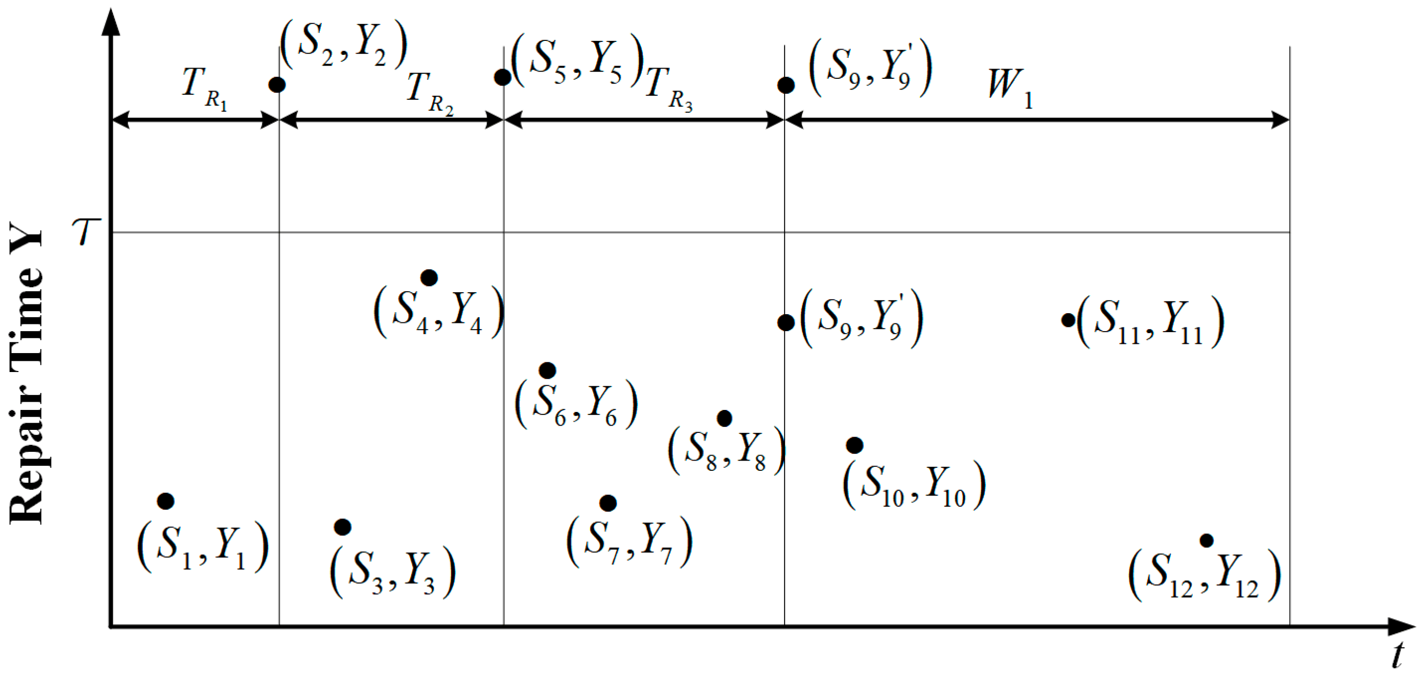
The general assumptions for the $\{\tau ,N\}$ and $\{\tau ,N_1,1\}$ models will be given in this section.

The operating process of the product can be modeled by a homogeneous discrete-state continuous-time Markov chain $\{X(t),t\ge 0\}$. The state space of the chain is $S=U\cup D=U\cup D_1\cup D_2$, where $U$ and $D$ are the subsets of working and failure states, respectively, and $D_1$ and $D_2$ are minor and catastrophic failure state sets, respectively.

The state transition probability matrix of the Markov process is $\mathit{Q}=[q_{ij}], i\in U, j\in U\cup D$ for $i\ne j$, $i\in U,j\in U\cup D$, and $q_{ij}$ is the transition rate from state $i$ to state $j$. The diagonal elements $q_{ii}$ are constructed such that the row sums are all zero, so that $q_{ii}$ is minus the sum of all rate constants leaving state $i$ and is therefore negative. If the system is in state $i$, the probability that the system transitions to state $j$ can be calculated by $q_{ij}/(-q_{ii})$.

Note that $\mathit{Q}$ can be partitioned in various ways according to the problem under consideration; for example, $\mathit{Q}$ is commonly partitioned by the operating and failure states $U$ and $D$,

$$\mathit{Q}=(\begin{array}{cc}{\mathit{Q}}_{UU}& {\mathit{Q}}_{UD}\end{array})$$

where ${\mathit{Q}}_{UU}$ is the sub-matrix of transition rates among states in the working states set $U$ and ${\mathit{Q}}_{UD}$ is the one from the working states set $U$ to failure states set $D$. ${\mathit{Q}}_{UD}$ may be partitioned further according to the type of failure, such as:

$${\mathit{Q}}_{UD}=(\begin{array}{cc}{\mathit{Q}}_{U{D}_1}& {\mathit{Q}}_{U{D}_2}\end{array})$$

where ${\mathit{Q}}_{U{D}_1}$ and ${\mathit{Q}}_{U{D}_2}$ are the sub-matrices of transition rates from working states set $U$ to minor and catastrophic failure states sets, $D_1$ and $D_2$, respectively.

Throughout the paper, all the matrices and vectors are written in bold face. Furthermore, $\mathbf{I}$ denotes an identity matrix and $\mathit{e}$ denotes a column vector of ones, the dimensions of them being apparent from the context.

2.2. Assumptions of $\{\tau ,N\}$ Model

This section is devoted to the assumptions of the $\{\tau ,N\}$ model.

(1)

Consider a repairable product sold with a warranty period $W_1$ and the warranty is renewed according to the $\{\tau ,N\}$ mechanism. That is, it will be replaced with a new and identical one, and warranty terms are renewed at no charge to customers if the repair time for a failure (regardless of the failure type) is more than $\tau$ or the number of visits to the failure states set $D$ over the warranty period exceeds $N$. Suppose that the times for visiting the operating states set are independent random variables having finite expectations and they are also independent of the times for repair actions.

(2)

Let $\{Y_i, i=1,2,\cdots \}$ be the sequence of repair times. Suppose that $Y_1,Y_2,\cdots$ are independent and identically distributed random variables with a probability distribution $G(t)$ and finite expectation.

(3)

At the expiration of the renewable warranty terms, if a repair is in progress, it will be continued at no charge to the customer. Repair times are not included in the warranty period ([13]). Repair times, unless otherwise specified, are not part of the time that the product goes through in this paper.

Let $S_i(i=1, 2,\cdots )$ denote the time of the completion of the $i$th repair action. A possible product state evolution path for such a combined warranty term when $N=3$ is shown in Figure 1 ([10]).

In Figure 1, the repair time for the first failure does not exceed the threshold $\tau$, while the second one exceeds the threshold. Furthermore, the total time that the product goes through two failures does not exceed the warranty period $W_1$, so the product is replaced at time $S_2$ and the time for the first renewal of the warranty terms is $T_{R_1}$. Similarly, the product is replaced at the fifth failure and the duration between the first and second renewals is $T_{R_2}$. The repair times for the sixth failure, the seventh failure, and the eighth failure do not exceed the threshold $\tau$, but the number of failures exceeds the threshold 3; therefore, the warranty terms are renewed. During the following warranty period, the product goes through four failures and their repair times do not exceed the threshold, so the warranty terms are not renewed and the warranty service ends. The length of the whole warranty period is $T_{R_1}+T_{R_2}+T_{R_3}+W_1$ and 12 repairs are performed.

2.3. Probability Analysis of $\{\tau ,N\}$ Model

2.3.1. Renewable Warranty Service Analysis of $\{\tau ,N\}$ Model

Considering the possible causes of a warranty renewal, two cases, in which the number of visits to failure states set exceeds the threshold $N$ and the time for one repair action is longer than threshold $\tau$, are investigated and they are denoted Case 1–1 and Case 1–2.

For Case 1–1, a product has gone through $N$ repairs which take no more than $\tau$ (short repair) and transit to failure states set $D$ from the operating states set $U$ within $(0,W_1)$. Let ${\mathit{T}}^0$ be the time that the product has completed the above activities regardless of the threshold $W_1$ and $[f_{ij}^{}(t)]$ is the probability function of ${\mathit{T}}^0$ given the entry state $i$$(i\in U)$ and the exit state $j$$(j\in D)$. Assume that ${\mathit{\phi }}^0(s)=[{\phi }_{ij}^0(s)]$$(s\ge 0)$ is the Laplace transform matrix of ${\mathit{T}}^0(t)=[f_{ij}^0(t)]$ ($i\in U,j\in D$).

Proposition 1.

For a multi-state product with the failure process modeled by the homogeneous discrete-state continuous-time Markov chain $\{X(t)\}$ and the warranty terms renewed according to the $\{\tau ,N\}$ regulation, the Laplace transform of the time that the product has gone through $N$ short repairs and transited to failure states is:

$$\begin{array}{ll}{\phi }^0(s)=& ({\mathit{\mu }}_0{(s\mathbf{I}-{\mathit{Q}}_{UU})}^{-1}{\mathit{Q}}_{UD}{\mathit{P}}_{SDU}{\mathit{e}}_U)\times \\ & ({\mathit{\mu }}_1{({(s\mathbf{I}-{\mathit{Q}}_{UU})}^{-1}{\mathit{Q}}_{UD}{\mathit{P}}_{SDU})}^{N-1}{\mathit{e}}_U){\mathit{\mu }}_1{(s\mathbf{I}-{\mathit{Q}}_{UU})}^{-1}{\mathit{Q}}_{UD}{\mathit{e}}_D,\end{array}$$

(1)

where ${\mathit{\mu }}_0$ is the initial state probability vector, ${\mathit{\mu }}_1$ is the state probability vector after a repair action, and ${\mathit{P}}_{SDU}$ is the state transition probability matrix after a short repair.

Proof. 

Given the entry state in $U$ and the exit state in $D$, the Laplace transform matrix of duration time in $U$ is ${(s\mathbf{I}-{\mathit{Q}}_{UU})}^{-1}{\mathit{Q}}_{UD}$ (see [28]). According to the convolution property of the Laplace transform, ${(s\mathbf{I}-{\mathit{Q}}_{UU})}^{-1}{\mathit{Q}}_{UD}{\mathit{P}}_{SDU}$ is the Laplace transform matrix of the time for a cycle under which the time for each repair is smaller than $\tau$. Reusing the above results, Equation (1) can be obtained. □

Let $T^0(t)$ be the inverse Laplace transform of ${\phi }^0(s)$. The probability that the warranty term is renewed due to exceeding the threshold number of visits to the failure states sets is:

$$p_0={\displaystyle {\int }_0^{W_1}{T}^0(t)}\mathrm{d}tG{(\tau )}^N$$

(2)

For Case 1–2, the first $l-1\left(l=1,\cdots ,N\right)$ short repairs and the $l$th long repair (a repair action which takes more than $\tau$) are completed within $W_1$. Let ${\mathit{T}}^l$ be the time required to complete the above activities regardless of the threshold $W_1$ and $[f_{ij}^l(t)]$ be the probability function of ${\mathit{T}}^l$ given the entry state $i(i\in U)$ and the exit state $j j\in D)$. Assume that ${\mathit{\phi }}^l(s)=[{\phi }_{ij}^l(s)]$$(s\ge 0)$ is the Laplace transform matrix of ${\mathit{T}}^l(t)=[f_{ij}^l(t)]$($i\in U,j\in D$).

Proposition 2.

For a multi-state product with the failure process modeled by the homogeneous discrete-state continuous-time Markov chain $\{X(t)\}$ and the warranty terms renewed according to the $\{\tau ,N\}$ regulation, the Laplace transform of the time that the product has gone through $l-1\left(l=1,\cdots ,N\right)$ short repairs and a long repair is:

$$\begin{array}{ll}{\phi }^l(s)=& ({({\mathit{\mu }}_{0}s\mathbf{I}-{\mathit{Q}}_{UU})}^{-1}{\mathit{Q}}_{UD}{\mathit{P}}_{SDU}{\mathit{e}}_U)({\mathit{\mu }}_1{({(s\mathbf{I}-{\mathit{Q}}_{UU})}^{-1}{\mathit{Q}}_{UD}{\mathit{P}}_{SDU})}^{l-2}{\mathit{e}}_U)\times \\ & {\mathit{\mu }}_1{(s\mathbf{I}-{\mathit{Q}}_{UU})}^{-1}{\mathit{Q}}_{UD}{\mathit{P}}_{LDU}{\mathit{e}}_U, l=2,\cdots ,N,\end{array}$$

(3)

$${\phi }^1(s)={\mathit{\mu }}_0{(s\mathbf{I}-{\mathit{Q}}_{UU})}^{-1}{\mathit{Q}}_{UD}{\mathit{P}}_{LDU}{\mathit{e}}_U.$$

(4)

where  ${\mathit{P}}_{LDU}$ is the state transition probability matrix after a long repair.

Proposition 2 can be proved in a similar manner as Proposition 1.

Let $T^l(t)(l=1,\cdots ,N)$ be the inverse Laplace transform of ${\phi }^l(s)$. Given the number of short repairs $l$, the probability that the warranty term is renewed is:

$$p_l={\displaystyle {\int }_0^{W_1}{T}^l(t)}\mathrm{d}tG{(\tau )}^{l-1}(1-G(\tau )), l=1,\cdots ,N$$

(5)

Let $p_{\tau N}$ be the warranty renewal probability under the $\{\tau ,N\}$ model. Then:

$$p_{\tau N}={\displaystyle \sum _{l=0}^N{p}_l}$$

The expected length of a renewable warranty for Case 1–1 is:

$$L_0=\frac{{\displaystyle {\int }_0^{W_1}t}{T}^0(t)\mathrm{d}t}{p_{\tau N}}.$$

(6)

The expected length of a renewable warranty under Case 1–2 is:

$$L_l=\frac{{\displaystyle {\int }_0^{W_1}t}{T}^l(t)\mathrm{d}t}{p_{\tau N}}, l=1,\cdots ,N.$$

(7)

Note that after the product has gone through $N$ short-duration repairs and transits to the failure states set $D$ from the operating states set $U$ within $W_1$, the warranty term will be renewed immediately under the obligation. Therefore, it is impossible that the warranty term is renewed due to exceeding the number of visits to the failure states set and the repair time.

2.3.2. Nonrenewable Warranty Service Analysis of $\{\tau ,N\}$ Model

According to the modeling assumptions, if the warranty term is not renewed, the product can visit the working state set $l\left(l=1,\cdots ,N+1\right)$ times and $l\left(l=0,\cdots ,N\right)$ short repairs can happen over the warranty period.

The Laplace transform for the probability density functions of $l(l=1,\cdots ,N)$ visits to the working state set and $l$ short repairs is

$${\phi }^l(s)=({\mathit{\mu }}_0{(s\mathbf{I}-{\mathit{Q}}_{UU})}^{-1}{\mathit{Q}}_{UD}{\mathit{P}}_{SDU}{\mathit{e}}_D){({\mathit{\mu }}_1{(s\mathbf{I}-{\mathit{Q}}_{UU})}^{-1}{\mathit{Q}}_{UD}{\mathit{P}}_{SDU}{\mathit{e}}_D)}^{l-1}.$$

(8)

The associated probability density functions are denoted by $f_l\left(t\right)$.

Proposition 3.

The probability that the product has gone through $l\left(l=0,\cdots ,N\right)$ short repairs over the warranty period, no repair action is performed, and warranty terms are not renewed is:

$${\tilde{p}}_l=\left({\displaystyle {\int }_0^{W_1}{\displaystyle {\int }_{W_1-t_1}^{+\infty }{f}_l(t_1)f(t_2)d{t}_1}d{t}_2}\right)G^l(\tau ), l=1,\cdots ,N,$$

(9)

$${\tilde{p}}_0={\displaystyle {\int }_{W_1}^{+\infty }{f}_1(t_1)d{t}_1}.$$

(10)

where $f(t_2)$ is the inverse Laplace transform of ${\mathit{\mu }}_1{(s\mathbf{I}-{\mathit{Q}}_{UU})}^{-1}{\mathit{Q}}_{UD}{\mathit{e}}_D$.

Proof. 

If the warranty term is not renewed and no repair action is performed, the duration in $U$ will be longer than $W_1$, which gives Equation (9). If warranty term is not renewed and $l\left(l=0,\cdots ,N\right)$ short repairs are performed during the warranty period, then the time taken by the $l(l=0,\cdots ,N)$ cycles will be shorter than $W_1$ and the total time of the $l$ cycles and the following visits to the working state set is longer than $W_1$. According to the property of convolution, Equation (10) can be obtained. □

2.4. Cost Analysis of $\{\tau ,N\}$ Model

In this section, the cost rate of the $\{\tau ,N\}$ model will be given.

According to the assumptions in Section 2.2, the warranty terms would be renewed if the number of visits to the failure states set $D$ is more than $N$ or the repair time of a failure (regardless of the failure type) is more than $\tau$ within the warranty period; otherwise the warranty policy would not be renewed and the warranty period will end with the warranty services over $(0,W_1)$. After the last repair of a renewable warranty, the old product has residual value $c_s$. The cost of updating a product is $c_{nw}^{}(c_{nw}^{}>c_s^{})$.

Let $W_{\{\tau ,N\}}$ denote the length of the warranty under the $\{\tau ,N\}$ regulation. It is clear that $W_{\{\tau ,N\}}$ is a random variable depending on the total number of warranty renewals, the inter-arrival times between two successive renewals of the warranty terms, and the length of the original warranty period $W_1$. Hence,

$$W_{\{\tau ,N\}}=T_{R_1}+T_{R_2}+\cdots +T_{R_{N_R}}+W_1,$$

(11)

where $N_R$ is the number of renewals during the warranty period, $T_{R_i}(i=1,\cdots ,N_R)$ are the time intervals between two subsequent warranty renewals, and they are independent and identically distributed non-negative random variables.

Theorem 1.

For a multi-state product with the failure process modeled by the homogeneous discrete-state continuous-time Markov chain $\{X(t)\}$ and warranty terms renewed according to the $\{\tau ,N\}$ regulation, the expected length of the warranty service is:

$$E(W_{\tau ,N})=\frac{{\displaystyle \sum _{l=0}^N{p}_i{L}_i}}{1-p_{\tau N}}+W_1.$$

(12)

Proof. 

According to the assumptions in Section 2.2, the probability that the warranty terms are renewed is $p_{\tau N}={\displaystyle {\sum }_{l=0}^N{p}_l}$. If the product is renewed, the expected inter-arrival times between two successive renewals is:

$$E(T_{R_1})=\frac{1}{p_{\tau N}}{\displaystyle \sum _{l=0}^N{p}_l}{L}_l.$$

(13)

□

The probability that the warranty terms are renewed $s$ times is:

$$P(N_R=s)=p_{\tau N}{}^s(1-p_{\tau N}),s=0,\cdots .$$

(14)

Given $N_R=s$, the expected length of the warranty service is:

$$E(W_{\{\tau ,N\}}\left|N_R=s)\right.=E(T_{R_1}+T_{R_2}+\cdots +T_{R_s}+W_1)=\frac{s}{p_{\tau N}}{\displaystyle \sum _{l=0}^N{p}_l{L}_l}+W_1.$$

(15)

By taking the expectation for the conditional expectation of Equation (15) with respect to  $N_R$,

$$\begin{array}{ll}E(W_{\{\tau ,N\}})& =E(E(W_{\{\tau ,N\}}\left|N_R)\right.\\ & ={\displaystyle \sum _{s=0}^{+\infty }E}(W_{W_{\{\tau ,N\}}}\left|N_R=s)P(N_R=s)\right.\\ & ={\displaystyle \sum _{s=0}^{+\infty }(\frac{s}{p_{\tau N}}{\displaystyle \sum _{l=0}^N{p}_l{L}_l}+W_1)}{p}_{\tau N}{}^s(1-p_{\tau N})\\ & =\frac{{\displaystyle \sum _{l=0}^N{p}_l{L}_l}}{1-p_{\tau N}}+W_1.\end{array}$$

(16)

Let $C_{\{\tau ,N\}}$ denote the total cost of the warranty service under the $\{\tau ,N\}$ regulation. Then,

$$C_{\{\tau ,N\}}=C_{R_1}+C_{R_2}+\cdots +C_{R_{N_R}}+C_{W_1},$$

(17)

where $C_{R_i}(i=1,\cdots ,N_R)$ is the cost of the $i$th warranty renewal and they are independent and identically distributed non-negative random variables. $C_{W_1}$ is the warranty service cost during the nonrenewable warranty period $W_1$.

Theorem 2.

For a multi-state product with the failure process modelled by the homogeneous discrete-state continuous-time Markov chain $\{X(t)\}$ and warranty terms renewed according to the $\{\tau ,N\}$ regulation, the expected renewable warranty service cost over the warranty period is:

$$E(C_{\{\tau ,N\}}^{rw})=\frac{p_{0}N{c}_{nr}^s+{\displaystyle \sum _{l=1}^N{p}_l((l-1)c_{nr}^s+}{c}_{nr}^l)+p_{\tau N}(c_{nw}-c_s)}{1-p_{\tau N}},$$

(18)

where $c_{nr}^s$ and $c_{nr}^l$ are the cost for one short repair and long repair, respectively.

Proof. 

If the product is renewed, the expected warranty service cost over two successive renewals is:

$$E(C_{R_i})=\frac{1}{p_{\tau N}}[p_{0}N{c}_{nr}^s+{\displaystyle \sum _{l=1}^N{p}_l((l-1)c_{nr}^s+}{c}_{nr}^l)+p_{\tau N}(c_{nw}-c_s)].$$

(19)

□

In a similar manner to that of Equation (16), Equation (18) can be obtained.

The expected warranty service cost over the whole warranty period is:

$$E(C_{\{\tau ,N\}})=\frac{1}{1-p_{\tau N}}[p_{0}N{c}_{nr}^s+{\displaystyle \sum _{l=1}^N{p}_l((l-1)c_{nr}^s+}{c}_{nr}^l)+p_{\tau N}(c_{nw}-c_s)]+{\displaystyle \sum _{l=1}^N{\tilde{p}}_{l}l}{c}_{nr}^s,$$

(20)

The last term in Equation (19) is the cost for the nonrenewable warranty service. Combining with Equation (18), we obtain the average cost of the whole warranty period, which can be expressed as Equation (20).

From Equations (16) and (20), the expected cost rate per unit time during the warranty period can be given as follows:

$$C{R}_{\{\tau ,N\}}=E(C_{\{\tau ,N\}})/E(W_{\{\tau ,N\}}).$$

(21)

3. Assumptions and Probability Analysis of {τ, N₁, 1} Model

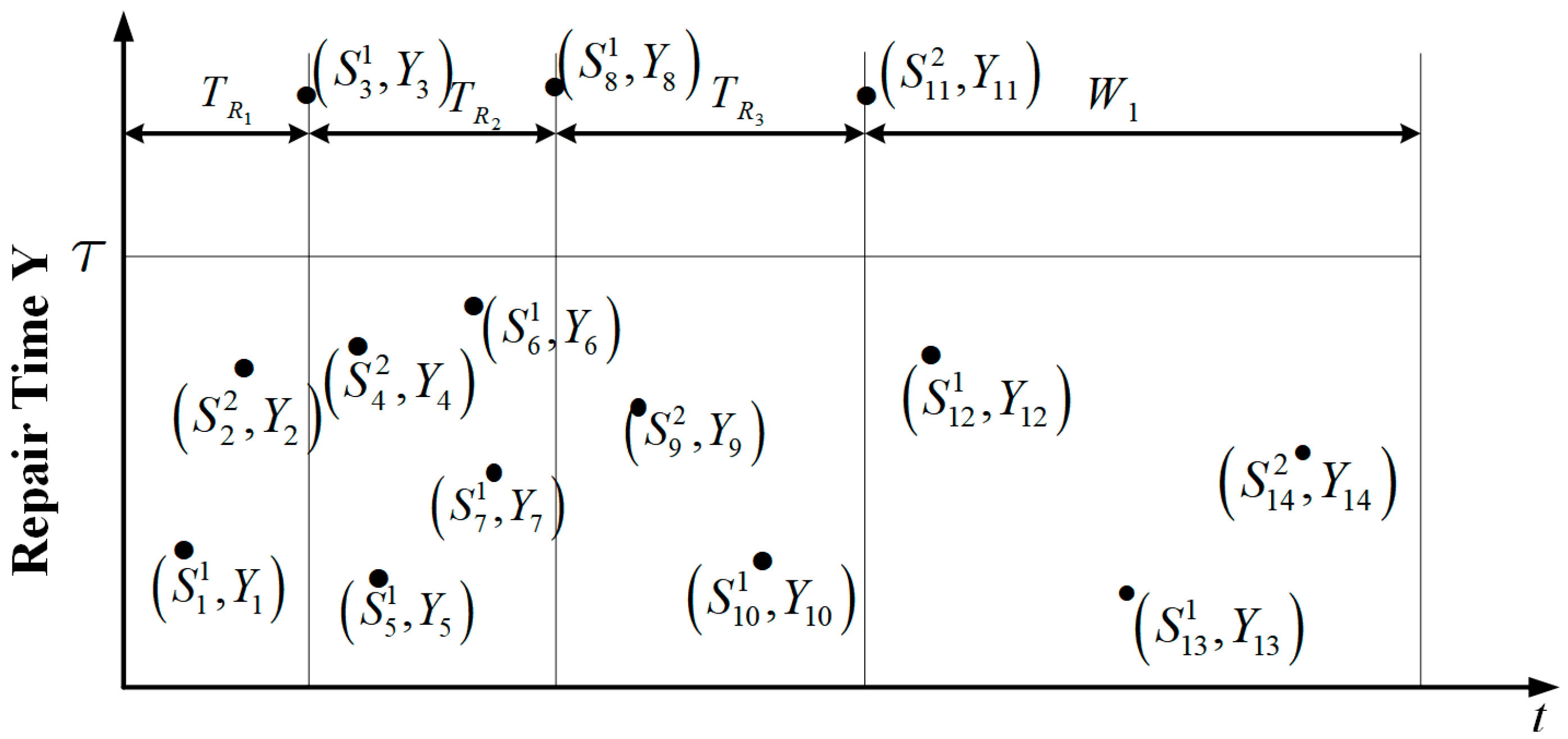
The assumptions and probability analysis of the $\{\tau ,N_1,1\}$ model will be given in the following.

3.1. Assumptions of $\{\tau ,N_1,1\}$ Model

Consider a repairable product sold with a warranty period $W_1$ with the warranty renewed according to the $\{\tau ,N_1,1\}$ model. Under the proposed $\{\tau ,N_1,1\}$ model, within the warranty period $W_1$, the product will be replaced with a new and identical one and the warranty will be renewed at no charge to the customer if the repair time of a failure (regardless of the failure type) is more than $\tau$, the number of visits to the minor failure states set $D_1$ is more than $N_1$, or the number of visits to the catastrophic failure states set $D_2$ is more than 1. Suppose that the lengths of visits to the operating states set are independent random variables having finite expectations, and they are independent from the repair times for minor failures and catastrophic failures.

Assumptions (1) and (2) of the $\{\tau ,N\}$ model are also made for the $\{\tau ,N_1,1\}$ model.

Let $S_i^1/S_i^2(i=1, 2,\cdots )$ denote the time for the $i$th repair completion of a minor failure/catastrophic failure. A possible product state evolution path for such a combined warranty term under $N_1=3$ is shown in Figure 2.

In Figure 2, the first renewal happens due to the ultra-limit of repair time. In the second and third renewals, the numbers of visits to the minor failure states set and catastrophic failure states set are higher than their thresholds 3 and 1, respectively. During the following warranty period, both the times and numbers of visits to the minor (catastrophic) failure states do not exceed the thresholds, and hence the warranty term is not renewed.

3.2. Probability Analysis of $\{\tau ,N_1,1\}$ Model

3.2.1. Renewable Warranty Analysis of $\{\tau ,N_1,1\}$ Model

According to the modeling assumptions, three cases—renewal due to the over-limit of catastrophic failures, minor failures, and repair time—are considered and they are denoted Case 2–1, Case 2–2, and Case 2–3, respectively.

For Case 2–1, the product has gone through one short duration in $D_2$, $m\left(m=1,\cdots ,N_1\right)$ times short duration in $D_1$, and transits to the catastrophic failure states set $D_2$ from the operating states set $U$ within $W_1$. Let $T_{ij}^{mk}$ be the time to complete the above activities regardless of the threshold $W_1$, given the total number of visits to the minor failures set $m(m=0,\cdots ,N_1)$, the serial number of visits to the catastrophic failures set $k(k=1,\cdots ,m+1)$, the entry state $i$$(i\in U)$, and the exit state $j$$(j\in D_2)$. $h_{ij}^{mk}$ is the probability function of $T_{ij}^{mk}$. Assume that ${\mathit{\varphi }}^{mk}(s)=[{\varphi }_{ij}^{mk}(s)](s\ge 0)$ is the Laplace transform matrix of ${\mathit{h}}_{}^{mk}(t)=[h_{ij}^{mk}(t)]$($i\in U,j\in D_2$).

Proposition 4.

For a multi-state product with the failure process modeled by the homogeneous discrete-state continuous-time Markov chain $\{X(t)\}$ and warranty terms renewed according to the $\{\tau , N_1,1\}$ regulation, the Laplace transform of the time that the product has gone through $m\left(m=1,\cdots ,N_1\right)$ short repairs due to minor failures, one catastrophic failure in the $kth(k=1,\cdots ,m+1)$ cycle, and transits to catastrophic failure states is:

$$\begin{array}{ll}{\varphi }^{m1}(s)=& ({\mathit{\mu }}_0{\mathit{G}}_{U{D}_2}(s){\mathit{P}}_{S{D}_{2}U}{\mathit{e}}_U){({\mathit{\mu }}_1{\mathit{G}}_{U{D}_1}(s){\mathit{P}}_{S{D}_{1}U}{\mathit{e}}_U)}^m\times \\ & ({\mathit{\mu }}_1{\mathit{G}}_{U{D}_2}(s){\mathit{e}}_{D_2}), m=0,\cdots ,N_1.\end{array}$$

(22)

$$\begin{array}{ll}{\varphi }^{mk}(s)=& ({\mathit{\mu }}_0{\mathit{G}}_{U{D}_1}(s){\mathit{P}}_{S{D}_{1}U}{\mathit{e}}_U){({\mathit{\mu }}_1{\mathit{G}}_{U{D}_1}(s){\mathit{P}}_{S{D}_{1}U}{\mathit{e}}_U)}^{k-2}\times \\ & ({\mathit{\mu }}_1{\mathit{G}}_{U{D}_2}\left(s\right){\mathit{P}}_{S{D}_{2}U}{\mathit{e}}_U\left)\right({\mathit{\mu }}_1{\mathit{G}}_{U{D}_1}(s){\mathit{P}}_{S{D}_{1}U}{\mathit{e}}_U{)}^{m-(k-1)}\times \\ & ({\mathit{\mu }}_1{\mathit{G}}_{U{D}_2}(s){\mathit{e}}_{D_2}), k=2,\cdots ,m,\hspace{0.33em}m=2,\cdots ,N_1.\end{array}$$

(23)

$$\begin{array}{ll}{\varphi }^{mm+1}(s)=& ({\mathit{\mu }}_0{\mathit{G}}_{U{D}_1}(s){\mathit{P}}_{S{D}_{1}U}{\mathit{e}}_U){({\mathit{\mu }}_1{\mathit{G}}_{U{D}_1}(s){\mathit{P}}_{S{D}_{1}U}{\mathit{e}}_U)}^{m-1}\times \\ & ({\mathit{\mu }}_1{\mathit{G}}_{U{D}_2}(s){\mathit{P}}_{S{D}_{2}U}{\mathit{e}}_U){\mathit{\mu }}_1{\mathit{G}}_{U{D}_2}(s){\mathit{e}}_{D_2}, m=1,\cdots ,N_1.\end{array}$$

(24)

where ${\mathit{G}}_{U{D}_1}(s)={(s\mathbf{I}-{\mathit{Q}}_{UU})}^{-1}{\mathit{Q}}_{U{D}_1},{\mathit{G}}_{U{D}_2}(s)={(s\mathbf{I}-{\mathit{Q}}_{UU})}^{-1}{\mathit{Q}}_{U{D}_2},$ ${\mathit{P}}_{S{D}_{1}U}$, and ${\mathit{P}}_{S{D}_{2}U}$ are the state transition probability matrixes after a short repair due to a minor failure and a catastrophic failure, respectively.

Proof. 

For $k=1$, during the first cycle, a catastrophic failure occurs and the repair time is not more than $\tau$; hence the Laplace transform for the probability density function of the first cycle’s length is ${\mathit{\mu }}_0{\mathit{G}}_{U{D}_2}(s){\mathit{P}}_{S{D}_{2}U}{\mathit{e}}_U$. During the following $m$ cycles, the product has goes through $m$ times of short duration in $D_1$, which gives the term ${({\mathit{\mu }}_1{\mathit{G}}_{U{D}_1}(s){\mathit{P}}_{S{D}_{1}U}{\mathit{e}}_U)}^m$. The last term ${\mathit{\mu }}_1{\mathit{G}}_{U{D}_2}(s){\mathit{e}}_{D_2}$ is the Laplace transform for the probability density function of the time that passes from the working state to the catastrophic failure set. Equations (23) and (24) can be proved in a similar manner. □

Let $h_{}^{mk}(t)$ be the inverse Laplace transform of ${\varphi }^{mk}(s)$. Given the number of visits to the minor failures set $m(m=0,\cdots ,N_1)$ and the serial number of visits to the catastrophic failures set $k(k=1,\cdots ,m+1)$, the probability that the warranty terms will be renewed is:

$$p_{mk}={\displaystyle {\int }_0^{W_1}{h}^{mk}(t)}\mathrm{d}tG{(\tau )}^{m+1}.$$

(25)

For Case 2–2, the product experiences 0 or 1 times of short duration in $D_2$, $N_1$ times of short duration in $D_1$, and transits to the minor failure set $D_1$ from the operating states set $U$ within $W_1$ times. Let $T_{ij}^0$ and $T_{kij}^1$ be the total times of the aforementioned process for the case that the product visits the catastrophic failure set 0 and 1 times, respectively, given the entry state $i$$(i\in U)$ and the exit state $j$$(j\in D)$. Assume that $h_{ij}^0(t)$ and $h_{kij}^1(t)$ are the probability density functions of $T_{ij}^0$ and $T_{kij}^1$, respectively, and ${\mathit{\varphi }}^0(s)=[{\varphi }_{ij}^0(s)] \mathrm{and} {\mathit{\varphi }}_k^1(s)=[{\varphi }_k^1(s)]$$(s\ge 0)$ are the Laplace transform matrices of ${\mathit{h}}^0(t)=[h_{ij}^0(t)]$ and ${\mathit{h}}_k^1(t)=[h_{kij}^1(t)]$, respectively.

Proposition 5.

For a multi-state product with the failure process modeled by the homogeneous discrete-state continuous-time Markov chain $\{X(t)\}$ and warranty terms renewed according to the $\{\tau ,N_1,1\}$ regulation, the Laplace transform of the time that the product has undergone $N_1$ short repairs due to minor failure, no or one catastrophic failure in the $kth(k=1,\cdots ,m+1)$ cycle, and a long repair due to a minor failure is:

$${\varphi }^0(s)=({\mathit{\mu }}_0{\mathit{G}}_{U{D}_1}(s){\mathit{P}}_{S{D}_{1}U}{\mathit{e}}_U){({\mathit{\mu }}_1{\mathit{G}}_{U{D}_1}(s){\mathit{P}}_{S{D}_{1}U}{\mathit{e}}_U)}^{N_1-1}{\mathit{\mu }}_1{\mathit{G}}_{U{D}_1}(s){\mathit{e}}_{D_1}.$$

(26)

$$\begin{array}{lll}{\varphi }_k^1(s)=& ({\mathit{\mu }}_0{\mathit{G}}_{U{D}_1}(s){\mathit{P}}_{S{D}_{1}U}{\mathit{e}}_U){({\mathit{\mu }}_1{\mathit{G}}_{U{D}_1}(s){\mathit{P}}_{S{D}_{1}U}{\mathit{e}}_U)}^{k-2}\times & \\ & ({\mathit{\mu }}_1{\mathit{G}}_{U{D}_2}(s){\mathit{P}}_{S{D}_{2}U}{\mathit{e}}_U\left)\right({\mathit{\mu }}_1{\mathit{G}}_{U{D}_1}(s){\mathit{P}}_{S{D}_{1}U}{\mathit{e}}_U{)}^{N_1-(k-1)}& {\mathit{\mu }}_1{\mathit{G}}_{U{D}_1}(s){\mathit{e}}_{D_1},\\ & & k=2,\cdots ,N_1,\end{array}$$

(27)

$${\varphi }_1^1(s)=({\mathit{\mu }}_0{\mathit{G}}_{U{D}_2}(s){\mathit{P}}_{S{D}_{2}U}{\mathit{e}}_U){({\mathit{\mu }}_1{\mathit{G}}_{U{D}_1}(s){\mathit{P}}_{S{D}_{1}U}{\mathit{e}}_U)}^{N_1-1} {\mathit{\mu }}_1{\mathit{G}}_{U{D}_1}(s){\mathit{e}}_{D_1}.$$

(28)

$$\begin{array}{ll}{\varphi }_{N_1+1}^1(s)=& ({\mathit{\mu }}_0{\mathit{G}}_{U{D}_1}(s){\mathit{P}}_{S{D}_{1}U}{\mathit{e}}_U){({\mathit{\mu }}_1{\mathit{G}}_{U{D}_1}(s){\mathit{P}}_{S{D}_{1}U}{\mathit{e}}_U)}^{N_1-1}\times \\ & ({\mathit{\mu }}_1{\mathit{G}}_{U{D}_2}(s){\mathit{P}}_{S{D}_{2}U}{\mathit{e}}_U){\mathit{\mu }}_1{\mathit{G}}_{U{D}_1}(s){\mathit{e}}_{D_1}.\end{array}$$

(29)

Equations (26)–(29) can be proved in a similar manner for Equation (22).

Let $h^0(t)$ and $h_k^1(t)\left(k=1,\cdots ,N_1+1\right)$ be the inverse Laplace transforms of ${\phi }^0(s)$ and ${\varphi }_k^1(s) (k=1,\cdots ,N_1+1)$, respectively. Then the probability that the warranty term is renewed due to exceeding the threshold number of visits to the minor failure set is:

$$p^0={\displaystyle {\int }_0^{W_1}{h}^0(t)}\mathrm{d}tG{(\tau )}^{N_1},$$

(30)

$$p_k^1={\displaystyle {\int }_0^{W_1}{h}_k^1(t)}\mathrm{d}tG{(\tau )}^{N_1+1},k=1,\cdots ,N_1+1,$$

(31)

For Case 2–3, the product experiences 0 or 1 catastrophic failures of short durations in $D_2$, $m$ short durations in $D_1$, and one longer duration in the failure set within $W_1$. Given the entry state $i$$(i\in U)$, the exit state $j$$(j\in D)$, and the serial number of visits to the catastrophic failures set, the times are denoted by $T_{mij}^0(m=0,\cdots ,N_1)$ and $T_{mkij}^1$, respectively. Let $h_{mij}^0(t)$ and $h_{mkij}^1(t)$ be the probability functions of $T_{mij}^0$ and $T_{mkij}^1$$(k=1,\cdots ,m+1)$, respectively. Assume that ${\mathit{\varphi }}_m^0(s)=[{\varphi }_{0ij}^0(s)] \mathrm{and} {\mathit{\varphi }}_{mk}^1(s)=[{\varphi }_{mk}^1(s)]\hspace{0.33em}(s\ge 0)$ are the Laplace transform matrices of ${\mathit{h}}_m^0(t)=[h_{mij}^0(t)]$ and ${\mathit{h}}_{mk}^1(t)=[h_{mkij}^1(t)]$.

Proposition 6.

For a multi-state product with the failure process modeled by the homogeneous discrete-state continuous-time Markov chain $\{X(t)\}$ and warranty term renewed according to the $\{\tau ,N_1,1\}$ regulation, the Laplace transform of the time that the product has undergone $m$ short repairs due to minor failure, no or one catastrophic failure in the $kth(k=1,\cdots ,m+1)$ cycle, and one longer repair is:

$${\varphi }_0^0(s)={\mathit{\mu }}_0{\mathit{G}}_{UD}(s){\mathit{P}}_{LDU}{\mathit{e}}_U,$$

(32)

$$\begin{array}{l}{\varphi }_m^0(s)=({\mathit{\mu }}_0{\mathit{G}}_{U{D}_1}(s){\mathit{P}}_{S{D}_{1}U}{\mathit{e}}_U){({\mathit{\mu }}_1{\mathit{G}}_{U{D}_1}(s){\mathit{P}}_{S{D}_{1}U}{\mathit{e}}_U)}^{m-1}({\mathit{\mu }}_1{\mathit{G}}_{UD}(s){\mathit{P}}_{LDU}{\mathit{e}}_U), \\ \hfill m=1,\cdots ,N_1-1.\end{array}$$

(33)

$${\varphi }_{N_1}^0(s)=({\mathit{\mu }}_0{\mathit{G}}_{U{D}_1}(s){\mathit{P}}_{S{D}_{1}U}{\mathit{e}}_U){({\mathit{\mu }}_1{\mathit{G}}_{U{D}_1}(s){\mathit{P}}_{S{D}_{1}U}{\mathit{e}}_U)}^{N_1-1}({\mathit{\mu }}_1{\mathit{G}}_{U{D}_2}(s){\mathit{P}}_{L{D}_{2}U}{\mathit{e}}_U).$$

(34)

$${\varphi }_{m1}^1=({\mathit{\mu }}_0{\mathit{G}}_{U{D}_2}(s){\mathit{P}}_{S{D}_{2}U}{\mathit{e}}_U){({\mathit{\mu }}_1{\mathit{G}}_{U{D}_1}(s){\mathit{P}}_{S{D}_{1}U}{\mathit{e}}_U)}^m({\mathit{\mu }}_1{\mathit{G}}_{U{D}_1}(s){\mathit{P}}_{L{D}_{1}U}{\mathit{e}}_U),$$

(35)

$$\begin{array}{ll}{\varphi }_{mk}^1=& ({\mathit{\mu }}_0{\mathit{G}}_{U{D}_1}(s){\mathit{P}}_{S{D}_{1}U}{\mathit{e}}_U){({\mathit{\mu }}_1{\mathit{G}}_{U{D}_1}(s){\mathit{P}}_{S{D}_{1}U}{\mathit{e}}_U)}^{k-2}\times \\ & ({\mathit{\mu }}_1{\mathit{G}}_{U{D}_2}(s){\mathit{P}}_{S{D}_{2}U}{\mathit{e}}_U\left)\right({\mathit{\mu }}_1{\mathit{G}}_{U{D}_1}(s){\mathit{P}}_{S{D}_{1}U}{\mathit{e}}_U{)}^{m-(k-1)}\times \\ & ({\mathit{\mu }}_1{\mathit{G}}_{U{D}_1}(s){\mathit{P}}_{L{D}_{1}U}{\mathit{e}}_U),k=2,\cdots ,m+1, m=1,2,\cdots ,N_1-1.\end{array}$$

(36)

$${\mathit{\varphi }}_{01}^1={\mu }_0{\mathit{G}}_{U{D}_2}(s){\mathit{P}}_{L{D}_{2}U}{\mathit{e}}_U.$$

(37)

In Equation (33), the product has experienced $m\hspace{0.33em}(m<N_1)$ short durations in $D_1$ and 0 visits to $D_2$; hence, the long duration may be in $D_1$ or $D_2$, which gives the term ${\mathit{\mu }}_1{\mathit{G}}_{UD}(s){\mathit{P}}_{LDU}{\mathit{e}}_U$. In Equation (34), the number of visits to $D_1$ reaches the threshold and the long duration would be in $D_2$, which gives the term ${\mathit{\mu }}_1{\mathit{G}}_{U{D}_2}(s){\mathit{P}}_{L{D}_{2}U}{\mathit{e}}_U$. Similarly, in Equations (35) and (36), the time of visits to $D_2$ reaches the threshold and the long duration would be in $D_1$, which gives the last term ${\mathit{\mu }}_1{\mathit{G}}_{U{D}_1}(s){\mathit{P}}_{L{D}_{1}U}{\mathit{e}}_U$. In Equation (37), the product has not experienced minor failures; therefore, the long duration would be the first visit to $D_2$.

Taking inverse Laplace transforms on Equations (32)–(37), the associated probability density functions can be given. The probabilities that the warranty terms are renewed due to exceeding the threshold repair time are as follows:

$$p_m^0={\displaystyle {\int }_0^{W_1}{h}_m^0(t)}\mathrm{d}tG{(\tau )}^m(1-G(\tau )),m=0,\cdots ,N_1-1,$$

(38)

$$p_{N_1}^0={\displaystyle {\int }_0^{W_1}{h}_{N_1}^0(t)}\mathrm{d}tG{(\tau )}^{N_1}(1-G(\tau )),$$

(39)

$$p_{mk}^1={\displaystyle {\int }_0^{W_1}{h}_{mk}^1(t)}\mathrm{d}tG{(\tau )}^{m+1}(G(\tau )), k=1,\cdots ,m+1, m=1,2,\cdots ,N_1-1,$$

(40)

$$p_{01}^1={\displaystyle {\int }_0^{W_1}{h}_{01}^1(t)}\mathrm{d}t(1-G(\tau )).$$

(41)

According to Equations (25), (30)–(31), and (38)–(41), the probability of warranty renewal under $\{\tau ,N_1,1\}$ is:

$$p_{\tau N_1}={\displaystyle \sum _{m=0}^{N_1}{\displaystyle \sum _{k=1}^{m+1}{p}_{mk}}}+p^0+{\displaystyle \sum _{k=1}^{N_1+1}{p}_k^1}+{\displaystyle \sum _{m=0}^{N_1}{p}_m^0}+{\displaystyle \sum _{m=1}^{N_1-1}{\displaystyle \sum _{k=1}^{m+1}{p}_{mk}^1}+}{p}_{01}^1.$$

The expected length of the renewed warranty under Case 2–1 is:

$$L_{mk}=\frac{{\displaystyle {\int }_0^{W_1}t}{h}^{mk}(t)\mathrm{d}t}{p_{\tau N_1}}, m=0,\cdots ,N_1, k=1,\cdots ,m+1.$$

(42)

The expected length of the renewed warranty for Case 2–2 is:

$$L^0=\frac{{\displaystyle {\int }_0^{W_1}t}{h}^0(t)\mathrm{d}t}{p_{\tau N_1}},$$

(43)

$$L_k^1=\frac{{\displaystyle {\int }_0^{W_1}t}{h}_k^1(t)\mathrm{d}t}{p_{\tau N_1}},k=1,\cdots ,N_1+1.$$

(44)

The associated expected lengths of the renewal warranty under Case 2–3 are denoted by $L_m^0\left(m=0,\cdots ,N_1-1\right)$, $L_{N_1}^0$, $L_{mk}^1\left(k=1,\cdots ,m+1,m=1,\cdots ,N_1-1\right)$, and $L_{01}^1$, respectively. They can be given in a similar manner to Equations (42)–(44).

3.2.2. Nonrenewable Warranty Service Analysis of $\{\tau ,N_1,1\}$ Model

According to the modeling assumptions, if warranty terms are not renewed under the $\{\tau ,N_1,1\}$ model, the product has undergone $m\hspace{0.33em}(l=0,\cdots ,N_1)$ short repairs due to minor failures and 0 or 1 catastrophic failure with short repairs over $(0,\hspace{0.33em}{W}_1)$.

The Laplace transform for the probability density function of the time that the product has gone without catastrophic failure, $m(m=1,\cdots ,N_1)$ times in the working state set, and $m(m=1,\cdots ,N_1)$ short repairs due to minor failures is:

$${\phi }_f^{0m}(s)=({\mathit{\mu }}_0{\mathit{G}}_{U{D}_1}(s){\mathit{P}}_{S{D}_{1}U}{\mathit{e}}_U){({\mathit{\mu }}_1{\mathit{G}}_{U{D}_1}(s){\mathit{P}}_{S{D}_{1}U}{\mathit{e}}_U)}^{m-1}.$$

(45)

The associated probability density functions are denoted by $f_m^0(t)$.

Laplace transforms for the probability density functions of the times that the product has experienced 1 short repair due to catastrophic failure at the $k$th cycle and $m(m=1,\cdots ,N_1)$ short repairs due to minor failure are given as:

$$\begin{array}{ll}{\phi }_{kf}^{1m}(s)=& {({\mathit{\mu }}_0{\mathit{G}}_{U{D}_1}(s){\mathit{P}}_{S{D}_{1}U}{\mathit{e}}_U)}^{k-1}({\mathit{\mu }}_1{\mathit{G}}_{U{D}_2}(s){\mathit{P}}_{S{D}_{2}U}{\mathit{e}}_U)\times \\ & ({\mathit{\mu }}_1{\mathit{G}}_{U{D}_1}(s){\mathit{P}}_{S{D}_{1}U}{\mathit{e}}_U{)}^{m-(k-1)}, k=1,\cdots ,m+1, m=1,2,\cdots ,N_1. \end{array}$$

(46)

$${\phi }_{1f}^{10}(s)={\mathit{\mu }}_0{\mathit{G}}_{U{D}_2}(s){\mathit{P}}_{S{D}_{2}U}{\mathit{e}}_U.$$

(47)

The associated probability density functions are denoted by $f_{mk}^1(t)$ and $f_{01}^1(t)$, respectively.

Using the same method as Proposition 3, we can obtain the following two propositions.

Proposition 7.

For a multi-state product with the failure process modeled by the homogeneous discrete-state continuous-time Markov chain $\{X(t)\}$ and warranty terms renewed according to the $\{\tau ,N_1,1\}$ regulation, the probability that the product has undergone $m(m=1,\cdots ,N_1)$ short repairs due to minor failures and the warranty terms are not renewed is:

$${\tilde{p}}_{{}_m}^0=\left({\displaystyle {\int }_0^{W_1}{\displaystyle {\int }_{W_1-t_1}^{+\infty }{f}_m^0\left(t_1\right)f\left(t_2\right)\mathrm{d}{t}_1}\mathrm{d}{t}_2}\right)G(\tau ), m=1,\cdots ,N_1.$$

(48)

where $f\left(t_2\right)$ is the inverse Laplace transform of ${\mathit{\mu }}_1{(s\mathbf{I}-{\mathit{Q}}_{UU})}^{-1}{\mathit{Q}}_{UD}{\mathit{e}}_D$.

Proposition 8.

For a multi-state product with the failure process modelled by the homogeneous discrete-state continuous-time Markov chain $\{X(t)\}$ and warranty terms renewed according to the $\{\tau ,N_1,1\}$ regulation, the probability that the product has undergone one short repair due to catastrophic failure at the $k$th cycle, $m(m=1,\cdots ,N_1)$ short repairs due to minor failures, and the warranty terms are not renewed is:

$${\tilde{p}}_{mk}^1=\left({\displaystyle \sum _{k=1}^{m+1}{\displaystyle {\int }_0^{W_1}{\displaystyle {\int }_{W_1-t_1}^{+\infty }{f}_{mk}^1(t_1)}}} f(t_2)\mathrm{d}{t}_1\mathrm{d}{t}_2\right)G{(\tau )}^{m+1},$$

(49)

$${\tilde{p}}_{01}^1=\left({\displaystyle {\int }_0^{W_1}{\displaystyle {\int }_{W_1-t_1}^{+\infty }{f}_{01}^1(t_1)}} f(t_2)\mathrm{d}{t}_1\mathrm{d}{t}_2\right)G(\tau ).$$

(50)

3.3. Cost Analysis of  $\{\tau ,N_1,1\}$ Model

Using the same method as that of Theorems 1 and 2, we can obtain the following two theorems.

Theorem 3.

For a multi-state product with the failure process modelled by the homogeneous discrete-state continuous-time Markov chain $\{X(t)\}$ and warranty terms renewed according to the $\{\tau ,N_1,1\}$ regulation, the expected length of the warranty service is:

$$E(W_{\{\tau ,N_1,1\}})=\frac{{\displaystyle \sum _{m=0}^{N_1}{\displaystyle \sum _{k=1}^{m+1}{p}_{mk}{L}_{mk}}}+p^0{L}^0+{\displaystyle \sum _{k=1}^{N_1+1}{p}_k^1{L}_k^1}+{\displaystyle \sum _{m=0}^{N_1}{p}_m^0{L}_m^0}+{\displaystyle \sum _{m=1}^{N_1-1}{\displaystyle \sum _{k=1}^{m+1}{p}_{mk}^1{L}_{km}^1}+}{p}_{01}^1{L}_{01}^1}{1-p_{\tau N_1}}+W_1.$$

(51)

Theorem 4.

For a multi-state product with the failure process modeled by the homogeneous discrete-state continuous-time Markov chain $\{X(t)\}$ and warranty terms renewed according to the $\{\tau ,N_1,1\}$ regulation, the expected warranty service costs over the renewable warranty period are:

$$\begin{array}{ll}E(C_{\{\tau ,N_1,1\}}^{rw})=\frac{1}{1-p_{\tau N_1}}& ({\displaystyle \sum _{m=0}^{N_1}{\displaystyle \sum _{k=1}^{m+1}{p}_{mk}(m{c}_{d_1}^s+c_{d_2}^s)}}+p^0{N}_1{c}_{d_1}^s+{\displaystyle \sum _{k=1}^{N_1+1}{p}_k^1(c_{d_2}^s+N_1{c}_{d_1}^s})+\\ & {\displaystyle \sum _{m=0}^{N_1-1}{p}_m^0}(m{c}_{d_1}^s+c_d^l)+p_{N_1}^0(N_1{c}_{d_1}^s+c_{d_2}^l)+{\displaystyle \sum _{m=1}^{N_1-1}{\displaystyle \sum _{k=1}^{m+1}{p}_{mk}^1(m{c}_{d_1}^s+c_{d_2}^s+c_{d_1}^l)}}+\\ & p_{01}^1{c}_{d_2}^l+p_{\tau N_1}(c_{nw}-c_s)),\end{array}$$

(52)

In Equation (52), $c_{d_1}^s$ and $c_{d_2}^s$ are the costs for short repairs of minor and catastrophic failures, respectively. $c_{d_1}^l$ and $c_{d_2}^l$ are the costs for long repairs of minor and catastrophic failures, respectively. $c_d^l$ is the cost for a long repair of a failure.

Similarly, the expected cost over the nonrenewable warranty period is:

$$E(C_{\{\tau ,N_1,1\}}^{nrw})={\displaystyle \sum _{m=1}^{N_1}{\tilde{p}}_m^{0}m{c}_{d_1}^s}+{\displaystyle \sum _{m=1}^{N_1}{\tilde{p}}_{mk}^1(m{c}_{d_1}^s+c_{d_2}^s)}+{\tilde{p}}_{01}^1{c}_{d_2}^s.$$

(53)

From Equations (51)–(53), the expected cost per unit time during the warranty period can be given as follows:

$$C{R}_{\{\tau ,N_1,1\}}=\frac{E(C_{\{\tau ,N_1,1\}}^{rw})+E(C_{\{\tau ,N_1,1\}}^{nrw})}{E(W_{\{\tau ,N_1,1\}})}.$$

(54)

4. Numerical Example

This section is devoted to two numerical examples for the $\{\tau ,N\}$ and $\{\tau ,N_1,1\}$ models.

4.1. Numerical Example for $\{\tau ,N\}$ Model

According to lemon laws in Pennsylvania, personal and family vehicles sold in the state will be recognized as defective if the number of repair actions exceeds three or the repair time for one repair exceeds 30 days over one year ([4]). Based on the aforementioned lemon laws, we consider the following example.

The multi-state product is renewed according to the {30,3} regulation. The whole warranty period $W_1=360$ days and the distribution function of repair time $G(t)=1-\exp (-\lambda t)$ with $\lambda =80$. The product has four working states and four failure states, i.e., 1, 2, 3, 4 and 5, 6, 7, 8, respectively. At the initial time, it is new, that is, ${\mathit{\mu }}_0=\left(\begin{array}{cccc}1& 0& 0& 0\end{array}\right)$. After repairs the product is restored to State 4, that is, ${\mathit{\mu }}_1=\left(\begin{array}{cccc}0& 0& 0& 1\end{array}\right)$. The state transit rate matrices of the failure process are:

$${\mathit{Q}}_{UU}=\left[\begin{array}{cccc}\begin{array}{c}-7.8\\ 3\\ 2.5\\ 2\end{array}& \begin{array}{c}2.5\\ -10.7\\ 3\\ 2.5\end{array}& \begin{array}{c}2\\ 2.5\\ -13\\ 3\end{array}& \begin{array}{c}1.5\\ 2\\ 2.5\\ -14.5\end{array}\end{array}\right], {\mathit{Q}}_{UD}=\left[\begin{array}{cccc}\begin{array}{c}1\\ 1.5\\ 2\\ 2.5\end{array}& \begin{array}{c}0.5\\ 1\\ 1.5\\ 2\end{array}& \begin{array}{c}0.2\\ 0.5\\ 1\\ 1.5\end{array}& \begin{array}{c}0.1\\ 0.2\\ 0.5\\ 1\end{array}\end{array}\right]$$

Since the product cannot be in the same state as the new product after a repair action (no matter short repair or long repair), ${\mathit{P}}_{SDU}$ and ${\mathit{P}}_{LDU}$ are set as follows:

$${\mathit{P}}_{SDU}=\left[\begin{array}{cccc}0& 0& 0.95& 0.05\\ 0& 0& 0.9& 0.1\\ 0& 0& 0.7& 0.3\\ 0& 0& 0.6& 0.4\end{array}\right],{\mathit{P}}_{LDU}=\left[\begin{array}{cccc}0& 0& 0.75& 0.25\\ 0& 0& 0.65& 0.35\\ 0& 0& 0.7& 0.3\\ 0& 0& 0.55& 0.45\end{array}\right].$$

Suppose that the residual value of the old product $c_s$ is $3000, the cost of updating the product $c_{nw}$ is $10,000, and the cost for a short repair and long repair are $300 and $1500, respectively.

According to the cost rate analysis in Section 2.3, the expected length of the warranty service is about 562 days and the expected warranty service cost over the whole warranty period is $11,954. The expected cost rate is $21.27 per day.

4.2. Numerical Example for $\{\tau ,N_1,1\}$ Model

According to the lemon laws in Virginia, pickup trucks, vans, and RVs sold will be recognized as defective if the number of repairs exceeds three, the time for a repair exceeds 30 days, or a catastrophic failure occurs during 18 months ([4]).

Based on the above facts, we set $\tau =30$$, N_1=3$, and $W_1=540$ days under the $\{\tau ,N_1,1\}$ model. States 5, 6 and States 7, 8 are minor and catastrophic failures, respectively. The other parameters are consistent with the $\{\tau ,N\}$ model. ${\mathit{Q}}_{UD}$ in Section 4.1 can be rewritten as:

$$\begin{array}{c}{\mathit{Q}}_{UD}=\left(\begin{array}{cc}{\mathit{Q}}_{U{D}_1}& {\mathit{Q}}_{U{D}_2}\end{array}\right)=\left[\begin{array}{cccc}1& 0.5& 0.2& 0.1\\ 1.5& 1& 0.5& 0.2\\ 2& 1.5& 1& 0.5\\ 2.5& 2& 1.5& 1\end{array}\right],\\ {\mathit{P}}_{SDU}={\mathit{P}}_{SDU}=\left(\begin{array}{c}{\mathit{P}}_{S{D}_{1}U}\\ {\mathit{P}}_{S{D}_{2}U}\end{array}\right)=\left[\begin{array}{cccc}0& 0& 0.95& 0.05\\ 0& 0& 0.9& 0.1\\ 0& 0& 0.7& 0.3\\ 0& 0& 0.6& 0.4\end{array}\right],{\mathit{P}}_{LDU}=\left(\begin{array}{c}{\mathit{P}}_{L{D}_{1}U}\\ {\mathit{P}}_{L{D}_{2}U}\end{array}\right)=\left[\begin{array}{cccc}0& 0& 0.75& 0.25\\ 0& 0& 0.65& 0.35\\ 0& 0& 0.7& 0.3\\ 0& 0& 0.55& 0.45\end{array}\right].\end{array}$$

When the product has undergone one short duration in $D_1$ or $D_2$, the costs for a repair $c_{d_1}^s$ and $c_{d_2}^s$ are $300 and $500, respectively. When the product has undergone one long duration in $D_1$ or $D_2$, the costs for a repair $c_{d_1}^l$ and $c_{d_2}^l$ are $1000 and $2000, respectively. Suppose that the cost for a long repair $c_d^l$ is $1500.

According to the cost rate analysis in Section 3.3, the expected warranty service duration is about 666 days, the expected warranty service cost over the entire warranty period is approximately $6514, and the expected cost rate per unit time during the warranty period is approximately $9.78 per day.

5. Conclusions

Many countries have enacted lemon laws to effectively protect the legitimate rights and interests of consumers. When a product subject to lemon laws is recognized as defective, manufacturers must bear the losses caused by quality problems. Therefore, from the point of view of manufacturers, the warranty cost analysis of these products is important for the design and quality control of the warranty strategy. Based on the terms of lemon laws, two warranty cost models, the $\{\tau ,N\}$ model and the $\{\tau ,N_1,1\}$ model, are proposed. Both consider the main characteristics of lemon laws: the limitations of the number of repair actions and the repair time over the warranty period. The $\{\tau ,N_1,1\}$ model focuses on products with minor and catastrophic failures. Numerical examples are given to illustrate the application of the models.

Warranty cost analysis in this paper is discussed under the assumptions that working times and repair times are independent and their expectations, Laplace and inverse Laplace transforms exist, which are suitable for low-dimensional models and restrict the applications of the results. In the future, we will consider the relevant theory and application problems.

The warranty cost analysis in this paper is discussed under the assumption of a renewable warranty, that is, a product that is recognized as defective will be replaced with a new and identical one and the warranty terms will also be updated accordingly. In certain lemon laws, warranties may be nonrenewable and manufacturers can refund to consumers the purchase cost partly or fully according to the deterioration level of the product. Cost analysis of nonrenewable warranty models with refunds is a future research direction. Other compensation methods, such as offering a free extended warranty service, need to be discussed. The design of the warranty policy and the optimization of products protected by lemon laws are also worthy of investigation.

References

1. Kegley, M.; Hiller, J. Emerging lemon car laws. Am. Bus. Law J. 1986, 24, 87–103. [Google Scholar] [CrossRef]
2. Husniah, H.; Pasaribu, U.; Iskandar, B. Warranty cost analysis for a multi- component product protected by lemon laws. IOP Conf. Ser. Mater. Sci. Eng. 2020, 1003, 012110. [Google Scholar] [CrossRef]
3. Guo, M. Introduction of Lemon Laws in American States (1). World Car 2002, 9, 27–28. (In Chinese) [Google Scholar]
4. Guo, M. Introduction of Lemon Laws in American States (2). World Car 2002, 10, 27–28+41. (In Chinese) [Google Scholar]
5. Wang, X.; He, K.; He, Z.; Li, L.; Xie, M. Cost analysis of a piece-wise renewing free replacement warranty policy. Comput. Ind. Eng. 2019, 135, 1047–1062. [Google Scholar] [CrossRef]
6. Wang, L.; Song, Y.; Pei, Z. Optimal condition-based warranty policy for multi-state products with three guarantees service. Qual. Technol. Quant. Manag. 2022, 19, 473–489. [Google Scholar] [CrossRef]
7. Husniah, H.; Wangsaputra, R.; Iskandar, B. Cost analysis of lemon law warranties for used equipments. Int. J. Artif. Intell. 2020, 18, 86–96. [Google Scholar]
8. Park, M.; Jung, K.; Park, D. Optimal post-warranty policy with repair time threshold for minimal repair. Reliab. Eng. Syst. Saf. 2013, 111, 147–153. [Google Scholar] [CrossRef]
9. Park, M.; Jung, K.; Park, D. Optimization of periodic preventive maintenance policy following the expiration of two-dimensional warranty. Reliab. Eng. Syst. Saf. 2018, 170, 233–245. [Google Scholar] [CrossRef]
10. Wang, L.; Pei, Z.; Zhu, H.; Lie, B. Optimising extended warranty policies following the two-dimensional warranty with repair time threshold. Eksploat. I Niezawodn. Maint. Reliab. 2018, 20, 523–530. [Google Scholar] [CrossRef]
11. Park, M.; Park, D. Two-dimensional Warranty Policy for Items with Refund Based on Korean Lemon Law. J. Appl. Reliab. 2018, 18, 349–355. [Google Scholar] [CrossRef]
12. Hooti, F.; Ahmadi, J.; Longobardi, M. Optimal extended warranty length with limited number of repairs in the warranty period. Reliab. Eng. Syst. Saf. 2020, 203, 107111. [Google Scholar] [CrossRef]
13. Liu, P.; Wang, G.; Su, P. Optimal maintenance strategies for warranty products with limited repair time and limited repair number. Reliab. Eng. Syst. Saf. 2021, 210, 107554. [Google Scholar] [CrossRef]
14. Zhao, X.; Chai, X.; Sun, J.; Qiu, Q. Joint optimization of mission abort and protective device selection policies for multistate systems. Risk Anal. 2022. [Google Scholar] [CrossRef] [PubMed]
15. Iscioglu, F. Dynamic performance evaluation of multi-state systems under non-homogeneous continuous time Markov process degradation using lifetimes in terms of order statistics. J. Risk Reliab. 2017, 231, 255–264. [Google Scholar] [CrossRef]
16. Li, M.; Kang, J.; Sun, L.; Wang, M. Development of optimal maintenance policies for offshore wind turbine gearboxes based on the non-homogeneous continuous-time Markov Process. J. Mar. Sci. Appl. 2019, 18, 93–98. [Google Scholar] [CrossRef]
17. Wang, L.; Jia, X.; Zhang, J. Reliability evaluation for multi-state Markov repairable systems with redundant dependencies. Qual. Technol. Quant. Manag. 2013, 10, 277–289. [Google Scholar] [CrossRef]
18. Wang, L.; Zhang, J.; Chen, W.; Jia, X. Reliability evaluation of a load-sharing parallel system with failure dependence. Commun. Stat. Simul. Comput. 2016, 45, 3094–3113. [Google Scholar] [CrossRef]
19. Du, S.; Zeng, Z.; Cui, L.; Kang, R. Reliability analysis of Markov history-dependent repairable systems with neglected failures. Reliab. Eng. Syst. Saf. 2017, 159, 134–142. [Google Scholar] [CrossRef] [Green Version]
20. Dong, F.; Liu, Z. Research on monitoring and Early warning of Product Warranty Claim based on ACUSUM. Ind. Eng. Manag. 2017, 22, 135–143. [Google Scholar]
21. Liao, H.; Cade, W.; Behdad, S. Markov chain optimization of repair and replacement decisions of medical equipment. Resour. Conserv. Recycl. 2021, 171, 105609. [Google Scholar] [CrossRef]
22. Hokstad, P.; Langseth, H.; Lindqvist, B.; Vatn, J. Failure modeling and maintenance optimization for railway line. Int. J. Perform. Eng. 2005, 1, 51–64. [Google Scholar]
23. Zhao, X.; Sun, J.; Qiu, Q.; Chen, K. Optimal inspection and mission abort policies for systems subject to degradation. Eur. J. Oper. Res. 2021, 292, 610–621. [Google Scholar] [CrossRef]
24. Zhao, X.; Fan, Y.; Qiu, Q.; Chen, K. Multi-criteria mission abort policy for systems subject to two-stage degradation process. Eur. J. Oper. Res. 2021, 295, 233–245. [Google Scholar] [CrossRef]
25. Qiu, Q.; Cui, L. Optimal mission abort policy for systems subject to random shocks based on virtual age process. Reliab. Eng. Syst. Saf. 2019, 189, 11–20. [Google Scholar] [CrossRef]
26. Qiu, Q.; Maillart, L.; Prokopyev, O.; Cui, L. Optimal Condition-Based Mission Abort Decisions. IEEE Trans. Reliab. 2022. [Google Scholar] [CrossRef]
27. Yang, L.; Chen, Y.; Qiu, Q.; Wang, J. Risk Control of Mission-Critical Systems: Abort Decision-Makings Integrating Health and Age Conditions. IEEE Trans. Ind. Inform. 2022, 18, 6887–6894. [Google Scholar] [CrossRef]
28. Colquhoun, D.; Hawkes, A. On the stochastic properties of the bursts of a single ion channel opening and of clusters of bursts. Philos. Trans. R. Soc. Lond. 1982, 300, 1–59. [Google Scholar]
Figure 1. A possible product state evolution path under  { τ , N } model.
Applsci 13 01541 g001
Figure 2. A possible product state evolution path under  { τ , N 1 , 1 } model.
Applsci 13 01541 g002
Disclaimer/Publisher’s Note: The statements, opinions and data contained in all publications are solely those of the individual author(s) and contributor(s) and not of MDPI and/or the editor(s). MDPI and/or the editor(s) disclaim responsibility for any injury to people or property resulting from any ideas, methods, instructions or products referred to in the content.