1. Introduction
Axial moving structures carry important technical meaning and present a series of engineering problems in industrial, mechanical, civil, aerospace, automotive, and electronics applications. In addition, such problems appear in the textile industry with thread lines, chain and belt drives, high-speed paper and tape, band saw blades, filament winding, filaments, aerial cable tracks, cooling tower battens, etc. Further, Wickert [
1] and Pellicano [
2] mentioned in their research on axially moving structures that, even at low speed, the axial velocity of the structure would significantly affect the dynamic characteristics of the structure, thus causing changes in the natural frequency and complex modes. However, when the critical axial velocity is exceeded, the engineering structure may suffer severe instability and coupled chatter, resulting in structural failure. Hence, accurate prediction of the dynamic characteristics and instability of such structures in advance is very important for successful analysis and optimization of the technical equipment design. So far, the differential equations of motion of axially moving beams have been solved by various means, including Galerkin’s method [
3], the assumed mode method [
4], the finite element method [
5,
6], Green’s function method [
7], the transfer function method [
8], the perturbation method [
9], the asymptotic method [
10], and the Laplace transform method [
11]. Lee et al. [
12] established a spectral element model of an axially moving Timoshenko beam under axially uniform tension. Then, the accuracy of the spectral element solution is verified by comparison with the conventional finite element solution and the exact analytical solution.
The FGM is a composite material whose properties vary continuously and smoothly from a ceramic surface to a metal surface in a specific structural direction. The ceramic surface protects the metal surface from corrosion and thermal damage, while the metal part provides strength and stiffness to the functionally graded material structure. Additionally, FGMs can be used in harsh environments with high temperatures. In this case, the use of FGMs can play a constructive role in extending the material service life. Currently, there have been considerable achievements made in the research on the mechanical behavior of FGMs and their components. Based on various beam theories, Mesut [
13] analyzed the dynamic characteristics of functionally graded beams under the action of moving loads. Further considering the transverse shear deformation, Yan et al. [
14] studied the dynamic response of functionally graded beams with boundary cracks on an elastic foundation under transverse loads of constant velocity. Liqun et al. [
15] studied the parametric vibration of an axially moving viscoelastic beam with varying velocity in the range of subharmonic resonance and combined resonance. Zhongmin et al. [
16] used the differential quadrature method to analyze the changes in the real and imaginary transverse vibration complex frequency of a functionally graded, simply supported beam in axial motion with parameters such as axial motion velocity and gradient index. However, in considering that the vibration of axially moving cantilever beams would affect the system’s safety and stability, Liang et al. [
17] analyzed the vibration characteristics of functionally graded cantilever beams. Haibo et al. [
18] analyzed the influences of axial force, axial force derivative, and motion acceleration on the inherent characteristics of the beam, and conducted a comparative study on the influencing factors such as critical load and critical velocity. The free and forced vibrations of an FG porous tube subjected to a moving, distributed load are investigated within the framework of a refined beam theory by Yuewu et al. [
19]. Subsequently, Yuewu et al. [
20] discuss the mechanical behaviors of an axially functionally graded (AFG) beam in microscales subjected to a moving mass. Based on Reddy’s shear deformation theory, Yuewu et al. [
21] developed for the first time a temperature-dependent GPL-reinforced porous beam model to explore the thermal buckling/postbuckling responses of beams.
In this paper, the transverse vibration mechanical properties of an axially moving FGM beam are studied under three boundary conditions: simply supported at two ends (SS), clamp supported at one end and simply supported at the other end (CS), and clamp supported at both ends (CC). Firstly, the displacement field and strain field of any point on the beam section are given based on the Euler-Bernoulli beam theory. In addition, according to the Hamilton principle, the free vibration motion differential equation of the axially moving FGM beam with the natural frequency as the eigenvalue is derived. Based on the basic theory of the interpolating matrix method (IMM) [
22,
23], the solution of the eigenvalue of the free vibration kinematic differential equation of an axially moving FGM beam is transformed into the solution of a set of eigenvalues of standard generalized algebraic equations by using an integral matrix. Finally, all the complex frequencies
Ω of transverse free vibration of an axially moving FGM beam are solved at once by orthogonal trigonometric decomposition (
QR). Meanwhile, the static divergence instability and dynamic coupling flutter characteristics of the axially moving FGM beam are studied.
2. Basic Theory and Calculation Formula
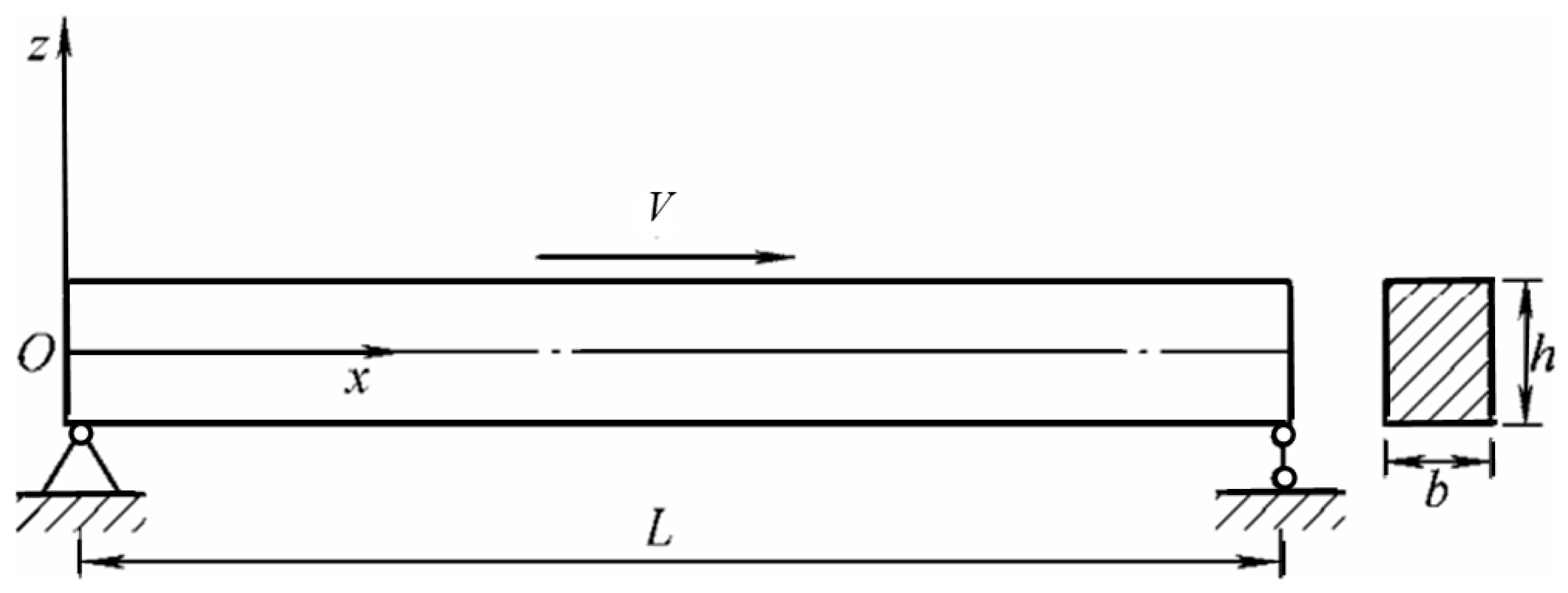
In a rectangular section beam, the elastic modulus
E(
z) and density
ρ(
z) of functionally graded materials change along the
z direction of height. Let beam length be
L, rectangular section height be
h, width be
b, and axial velocity be
V. Then, a rectangular coordinate system is established, as shown in
Figure 1. It is hypothesized that the FGM properties change along the
z direction of height according to the arbitrary functions
f(
z) and
g(
z), with the concrete expression shown as follows:
where, −
h/2 ≤
z ≤
h/2,
Em and
ρm are the elastic modulus and density of the reference material, respectively, and
f(
z) and
g(
z) are arbitrary functions with regard to coordinate
z. According to the Euler-Bernoulli beam theory, the displacement components
and
of any point on the beam in the directions
x and
z can be expressed as:
where,
u(
x,
t) and
w(
x,
t) are the axial displacement and transverse displacement of any point on the beam axis, respectively, and
Vt is the axial rigid body displacement generated by the axial motion velocity
V.
The strain energy
U of an axially moving FGM beam is,
The expressions of
γ0,
γ1, and
γ2 are respectively,
In Equation (6),
A =
bh,
S =
bh2/2,
I =
bh3/12, the same as below. In the transverse vibration of an axially moving FGM beam, the velocity of any point on the beam is,
The kinetic energy
K of the axially moving FGM beam is,
Here, the expressions for
I0,
I1, and
I2 are, respectively,
In Equation (10), the expressions for α
0, α
1, and α
2 are respectively,
According to the Hamilton principle
, due to the arbitrariness of the variable term, its coefficient of the variable term is zero [
18], thus,
By calculating the first-order partial derivatives of both sides of the equal sign in Equation (12) with regard to
x, the value
can be obtained as:
By substituting Equation (14) into Equation (13) for decoupling, the kinematic differential equation of axially moving FGM beam can be obtained,
The boundary conditions of a simply supported beam (SS) at both ends are [
24],
The boundary conditions of the clamp supported beam (CC) at both ends are,
The boundary conditions of a beam (CS) clamp supported at one end and simply supported at the other end are,
Here,
,
, the same as below. In order to facilitate the subsequent programming calculation, the following normalized variables are introduced.
By substituting Equation (17) into the motion differential Equation (15) of an axially moving FGM beam, there is
where,
Here,
λ is the length-height ratio of the FGM beam. If the axial motion velocity of the beam exceeds a certain critical value, the axially moving FGM beam may become unstable. In order to study the stability of the moving beam, it is usually hypothesized that the form of free vibration response is:
where,
Ω is the normalized complex frequency and
is the modal function. By substituting Equation (20) into Equation (18), we have:
The natural frequency
Ω of the complex form can be expressed in the following form:
The instability type of an axially moving FGM beam can be determined by the signs of the real part (Re) and imaginary part (Im) of all eigenvalues in Equation (21). Specifically, when Re(
Ω) = 0, Im(
Ω) ≠ 0, it is static stability; when Re(
Ω) ≠ 0, Im(
Ω) = 0, it is a static instability (divergence instability); and when Re(
Ω) ≠ 0, Im(
Ω) ≠ 0, it is a dynamic instability (coupled flutter). In order to facilitate the derivation and simplification of the following equations, let
By substituting Equation (22) into Equation (21), it can be simplified as,
The boundary conditions at both ends of the axially moving FGM beam after normalization are,
To sum up, the natural frequency calculation of the axially moving FGM beam is transformed into the solution of the eigenvalue of the ordinary differential Equation (23) under the boundary condition in Equation (24). Here, the interpolating matrix method is used for solution [
22,
23].
From a static state, with the increase of beam axial velocity, each order natural frequency of FGM beam decreases gradually. When the axial velocity reaches a certain value so that the first-order natural frequency disappears, the velocity is the critical velocity. If the FGM beam moves in the axial direction at a faster rate than this critical velocity, the beam will lose static stability. According to this law, in Equation (21), if we let
Ω = 0, then the governing equation for solving the critical velocity of the axially moving FGM beam is,
Thus, the interpolating matrix method (IMM) is used to solve the ordinary differential Equation (25) under the boundary condition in Equation (24), and the critical velocity of the axially moving FGM beam can be calculated.
3. Calculation of the Natural Frequency of an Axially Moving FGM Beam Using the Interpolating Matrix Method
The interpolating matrix method (IMM) [
22,
23] is an effective numerical calculation method for solving eigenvalues and two-point boundary values of ordinary differential equations. The method takes the highest derivative function in the ordinary differential equation as the unknown parameter of the discrete system. The solution of the eigenvalue of ordinary differential equations is transformed into the solution of the eigenvalue of standard generalized algebraic equation sets by means of an integral matrix.
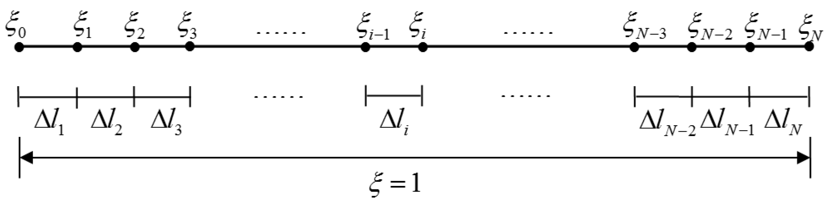
Figure 2 shows the calculation model of an axially moving FGM beam by the interpolating matrix method (IMM). The normalized interval [0,1] is divided into
N discrete elements, ξ
0 = 0, ξ
N= 1. The length of a discrete element is ∆
Li =
ξi-
ξi−1 = 1/
N, and the third derivative of an unknown function
in an ordinary differential Equation (26) is expressed by the function value of a discrete node on the beam length interval using the difference method.
The unknown derivative
in the above equation is approximated by the interpolating function, i.e.,
where,
Li(
ξ) is the basis function of lagrangian interpolation. In this paper, quadratic parabola interpolation is adopted, and its basis function is
By substituting Equations (27) and (28) into Equation (26), there is
Here,
is the integral matrix, which depends on the interpolation basic function
Li(
ξ). In order to facilitate the derivation of the following formulas, the following two (
N + 1)×1-order column vectors,
τ,
σ and an (
N + 1) × (
N + 1)-order unit matrix
I are introduced.
Equation (29) can be written in vector form as follows:
Here, , , ,
, .
If the lower derivatives in the system of ordinary differential equations are gradually replaced by higher derivatives, by recursion, there is
Here,
,
,
Here,
,
,
.
Here, , , .
The highest derivative
of the ordinary differential equation (in Equation (23)) can be written directly in vector form as follows:
Here, , ,
Equation (31) is substituted into Equation (23) and converted into matrix form as follows,
where,
.
Since Equation (32) contains
Ω2, which makes the eigenvalue solution of generalized algebraic equations nonlinear, a new (
N + 1) × 1-order column vector
is introduced to quasi-linearize Equation (32).
By substituting Equation (33) into Equation (32), we have:
By combining Equations (33) and (34) with the boundary condition in Equation (24), we have:
When the axially moving FGM beam is simply supported at both ends (SS), the vector form of the boundary condition is,
When the axially moving FGM beam is clamped at one end and simply supported at the other end (CS), the vector form of the boundary condition is,
When the axially moving FGM beam is clamped at both ends (CC), the vector form of the boundary condition is,
In Equation (36), and . are represented as the row elements of the matrix . The eigenvalue of a standard generalized algebraic equation set, such as Equation (35), can be solved by orthogonal trigonometric decomposition (QR). The method is the most effective and widely used method to solve all the eigenvalues of the matrix, which can obtain several orders of normalized complex frequency Ω and the corresponding modal function of an axially moving FGM beam at one time.
4. Numerical Examples and Problem Discussion
In order to solve a specific problem, suppose the axially moving FGM beam is made of ceramic and metal, and the elastic modulus
E(
z) and density
ρ(
z) of the material can be expressed as:
where
k is the material gradient index, the elastic modulus and density of metal materials are
Em = 210 GPa and
ρm = 7800 kg/m
3, respectively, and the elastic modulus and density of ceramic materials are
Ec = 390 GPa and
ρc = 3960 kg/m
3, respectively. When the functional gradient index of the beam material
k = 0 and
k = ∞, the functional gradient material beam degenerates into a uniform ceramic material beam and a metal material beam.
In order to verify the feasibility and accuracy of the interpolating matrix method (IMM) in solving the natural frequency in free vibration of the FGM beam, the length-height ratio of the FGM beam was set at
λ = 10, and the number of discrete elements
N = 6~22.
Table 1 shows the value of the dimensionless natural frequency of an axially moving FGM beam calculated by the interpolating matrix method (IMM). The value is compared with the results in the literature [
16]. The numerical results show that when the number of discrete beam length elements
N is greater than or equal to 12, the numerical results in this paper gradually converge to the actual value, and with the increase in the number of discrete elements
N, the interpolating matrix method (IMM) presents greater computational stability. The number of beam length discrete elements
N = 20.
Table 2 and
Table 3 illustrate the numerical solutions of the first three-order natural complex frequency using the interpolating matrix method (IMM) for a simply supported beam (SS) with material gradient index
k = 0.1 and 1.0 under different coaxial velocities
v, which are completely consistent with the calculated results of the existing literature [
16]. The feasibility and accuracy of the interpolating matrix method (IMM) in the analysis of transverse free vibration dynamics of axially moving FGM beams are thus further verified.
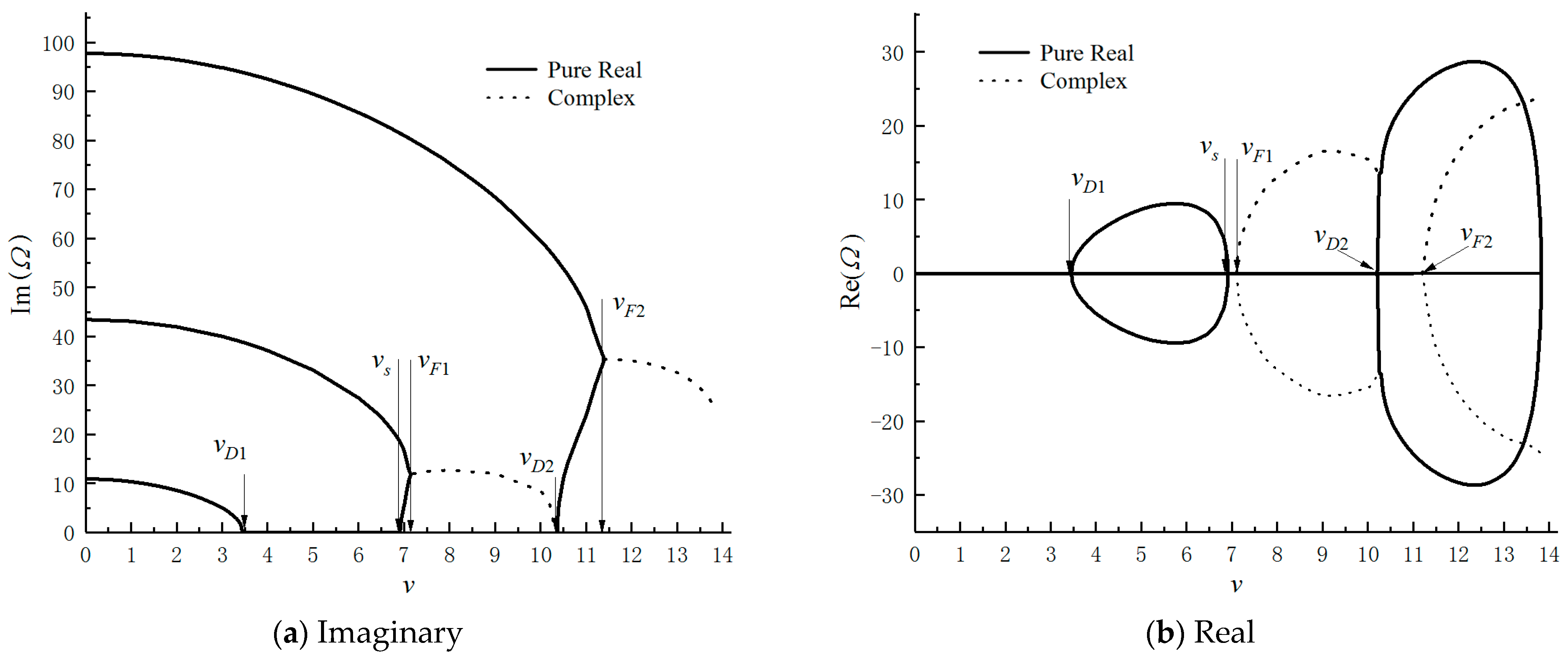
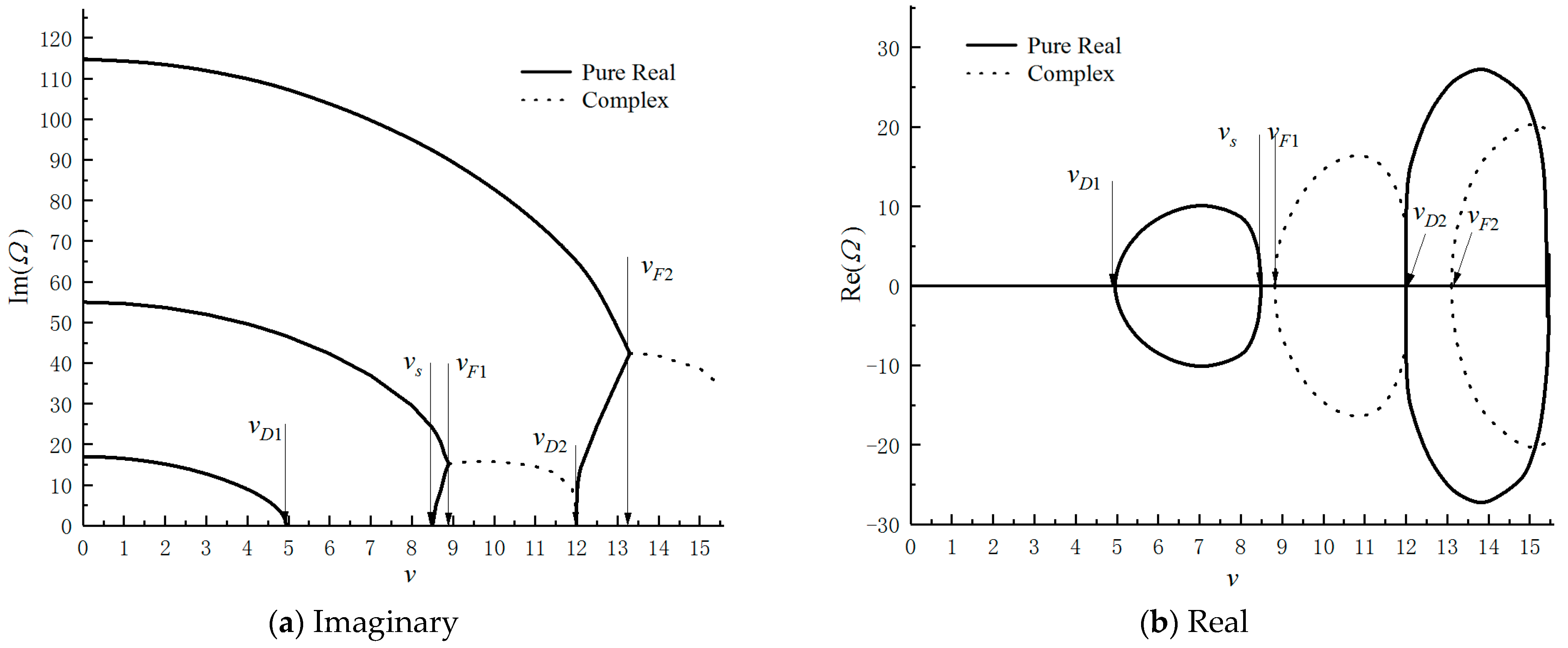
Figure 3,
Figure 4 and
Figure 5 show the change of the dimensionless natural complex frequency value Ω of an axially moving FGM beam with axial velocity
v when the FGM beam length-height ratio is
λ = 10, the material gradient index is
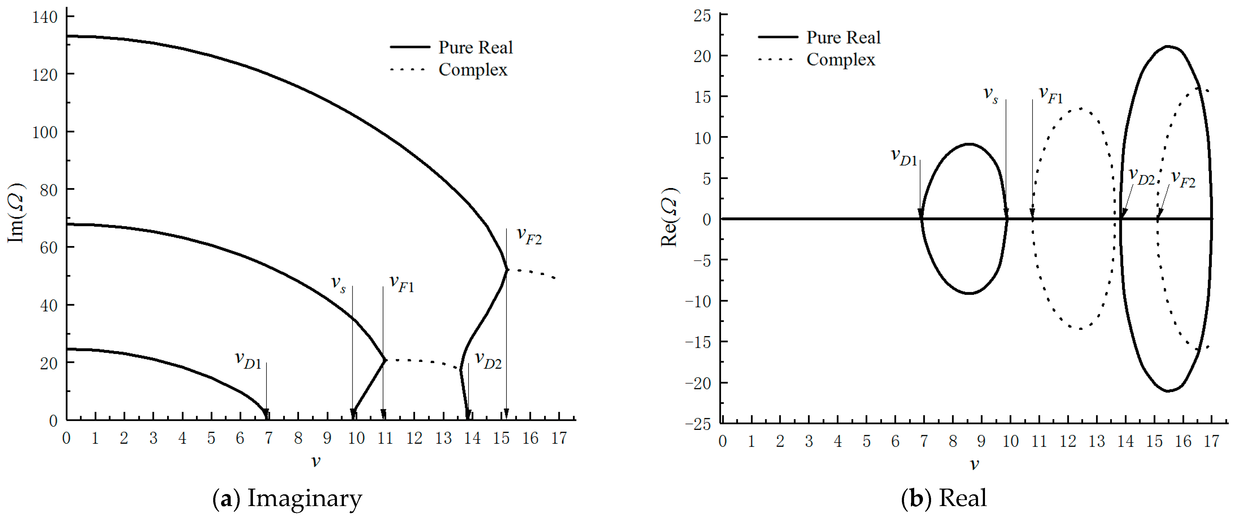
k = 10, and the boundary conditions are simply supported at both ends (SS), clamp supported at one end and simply supported at the other end (CS), and clamp supported at both ends (CC). When the dimensionless axial velocity is lower than
vD1 (
vD1 is the first dimensionless divergence velocity), i.e.,
v ≤
vD1, an axially moving FGM beam is stable because all the dimensionless natural frequency values
Ω are imaginary. However, if the dimensionless axial motion velocity is between
vD1 and
vs (
vs is the dimensionless axial motion velocity at the beginning of the second stability zone), that is, when
vD1 ≤
v ≤
vs, the first-order natural frequency
Ω1 is a real number, indicating the occurrence of static instability (i.e., divergence instability) of the beam.
Figure 3,
Figure 4 and
Figure 5 show that there is a very narrow second stable region between
vs and
vF1, that is, when
vs ≤
v ≤
vF1, all natural frequencies are imaginary. If the dimensionless axial velocity of the beam is greater than
vF1, that is, when
v ≥
vF1, then the first and second order dimensionless natural frequencies are a pair of complex conjugates, indicating that the beam has dynamic instability (that is, the first and second order coupled flutter). Therefore,
vF1 is the minimum coupled flutter velocity of the beam. In
Figure 3,
Figure 4 and
Figure 5,
vD2 is the second dimensionless divergence velocity, and
vF2 is the second dimensionless coupled flutter velocity. When
vD2 ≤
v ≤
vF2, it indicates the second occurrence of static instability of the beam (i.e., the second occurrence of divergence instability). When
v ≥
vF2, it indicates the second occurrence of dynamic instability (i.e., second- and third-order coupled flutter). The values of all critical axial velocities (
vD1,
vs,
vF1,
vD2, and
vF2) in
Figure 3,
Figure 4 and
Figure 5 calculated by the interpolating matrix method (IMM) are listed in
Table 4.
Table 5,
Table 6 and
Table 7 are the IMM calculated values of the dimensionless critical velocity when the gradient index of the functionally graded material is
k = 11~15. The calculation results show that with the increase of the material gradient index
k, the divergence velocity
vD1 and flutter velocity
vF1 of the axially moving FGM beam tend to decrease. The main reason is that when the material gradient index
k gradually increases from 0 to, ∞, the stiffness of the beam material gradually decreases.
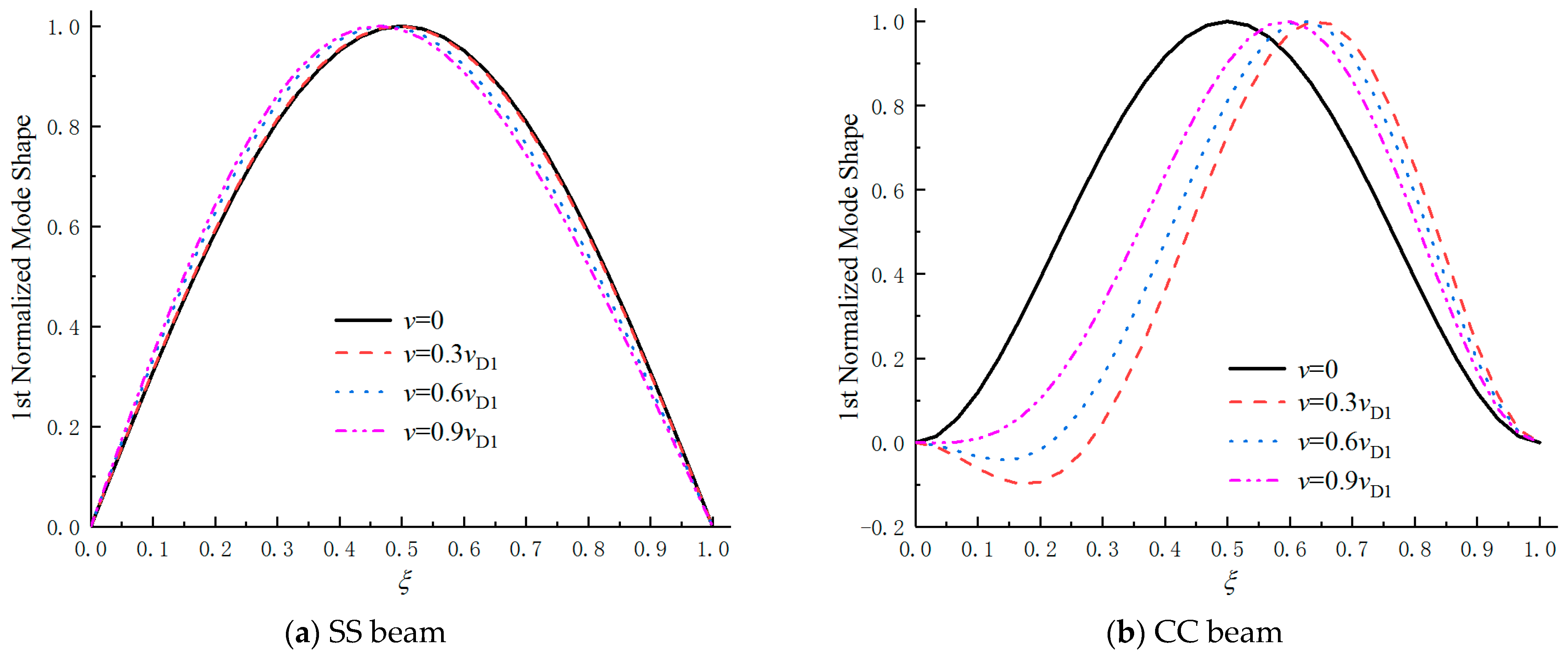
The modal function of an axially moving Euler-Bernoulli beam has a complex mode. In this paper, the interpolating matrix method (IMM) can not only be used to calculate the natural frequencies of several orders before the transverse free vibration of an axially moving FGM beam but also solve the corresponding modal function. Let the material gradient index
k = ∞, and then the FGM beam degenerates into a uniform metal beam.
Figure 6 compares the real part of the first-order mode of the uniform metal beam under different axial velocities (
v). The study found that the static SS beam and CC beam with symmetry in the first order mode are distorted due to the influence of the axial velocities
v. Therefore, the original symmetry of Euler-Bernoulli beams of uniform metal materials under static SS and CC boundary conditions cannot be applied to the case of axially moving beams, especially for beams with great axial velocities. Moreover, axial motion velocities exert a greater influence on the first-order modal distortion of a beam clamped at both ends (CC) compared to a beam simply supported at both ends (SS).
5. Conclusions
Based on the Euler-Bernoulli beam theory and the Hamilton principle, the transverse vibration kinematics control differential equation for an axially moving FGM beam is established. Based on the basic theory of the interpolating matrix method (IMM), the kinematic differential equation with an inherent complex frequency as an eigenvalue is converted into the eigenvalue solution of a standard generalized algebraic equation by using an integral matrix. Finally, the standard generalized algebraic equation set is solved by orthogonal trigonometric decomposition (QR), and the natural frequency of transverse vibration of an axially moving FGM beam is obtained. Meanwhile, the corresponding modal function is obtained. The main conclusions are drawn as follows:
(1) In this paper, the numerical calculation of the dimensionless natural complex frequency of axially moving FGM beams by the interpolating matrix method is in complete agreement with the results obtained in the previous findings, which verifies the calculation accuracy of the interpolating matrix method. At the same time, the numerical results show that, with the increase in the number of discrete elements on the beam length, the algorithm demonstrates strong computational stability.
(2) With the increase of material gradient index k, the divergence velocity and flutter velocity tend to decrease. When the axial velocity is equal to the lowest divergence velocity, vD1, the first-order natural frequency of the axially moving FGM beam disappears. That is, the first-order bending mode disappears, resulting in static instability. At the same time, there is a very narrow stability region between the first static instability region (divergence) and the first dynamic instability region (first- and second-order coupled chatter).
(3) In general, the beam clamp supported at both ends (CC) has the strongest constraint, while the beam simply supported at both ends (SS) has the weakest constraint. The calculation results of the interpolating matrix method (IMM) show that the divergence velocity and flutter velocity of an axially moving FGM beam tend to increase with the increase of boundary constraints.
(4) The axial velocity v causes symmetry distortion in the real part of the first-order complex mode of the simply supported beam (SS) and clamp supported beam (CC) with uniform metal material. The axial velocity v has a more significant effect on the real part distortion of the first order mode of the beam clamp supported at both ends (CC) compared to the beam simply supported at both ends (SS).


