Panchromatic and Multispectral Image Fusion Combining GIHS, NSST, and PCA

Abstract

Spatial and spectral information are essential sources of information in remote sensing applications, and the fusion of panchromatic and multispectral images effectively combines the advantages of both. Due to the existence of two main classes of fusion methods—component substitution (CS) and multi-resolution analysis (MRA), which have different advantages—mixed approaches are possible. This paper proposes a fusion algorithm that combines the advantages of generalized intensity–hue–saturation (GIHS) and non-subsampled shearlet transform (NSST) with principal component analysis (PCA) technology to extract more spatial information. Therefore, compared with the traditional algorithms, the algorithm in this paper uses PCA transformation to obtain spatial structure components from PAN and MS, which can effectively inject spatial information while maintaining spectral information with high fidelity. First, PCA is applied to each band of low-resolution multispectral (MS) images and panchromatic (PAN) images to obtain the first principal component and to calculate the intensity of MS. Then, the PAN image is fused with the first principal component using NSST, and the fused image is used to replace the original intensity component. Finally, a fused image is obtained using the GIHS algorithm. Using the urban, plants and water, farmland, and desert images from GeoEye-1, WorldView-4, GaoFen-7 (GF-7), and Gaofen Multi-Mode (GFDM) as experimental data, this fusion method was tested using the evaluation mode with references and the evaluation mode without references and was compared with five other classic fusion algorithms. The results showed that the algorithms in this paper had better fusion performances in both spectral preservation and spatial information incorporation.

1. Introduction

Spatial and spectral information are significant in remote sensing imaging applications, such as land classification, change detection, and road extraction. However, based on considerations of imaging quality, the high-frequency spatial information is separated from the spectral information during satellite imaging [1], and typical optical remote sensing satellites, such as QuickBird, WorldView-2, GF-1, and GF-2, only provide high-spatial-resolution panchromatic (PAN) images and low-spatial-resolution multispectral (MS) images. The fusion of PAN and MS images effectively solves the problem of this separation of the high-frequency spatial information from the spectral information.

According to the different techniques for high-frequency information injection, PAN-MS fusion can be divided into two categories: spectral and spatial methods [2]. The spectral methods are based on the component replacement method in which the spectral information component (SIC) is separated from the spatial structure component (SSC) by projecting the MS into another vector space. Then, the SSC is replaced by a PAN to incorporate high-frequency spatial information, and, finally, a fused image is obtained through inverse transformation. Typical component substitution (CS) methods include principal component analysis (PCA) and the Gram–Schmidt process (GS). In addition, in recent years, methods based on deep learning [3,4] have also achieved good results, but their computational complexity is high, and they are not suitable for large-scale remote sensing images; thus, this paper does not discuss them in depth.

The spatial methods include multi-resolution analysis (MRA), which decomposes MS and PAN at multiple scales. The high-frequency components are fused with low-frequency components using different rules and, finally, inverted back to the fused image. Typical MRA methods include wavelet transform [5], curvelet transform [6], contourlet transform [7,8], non-subsampled contourlet transform (NSCT) [9], non-subsampled shearlet transform (NSST) [10], and so on. Among these, wavelet transform is the most widely used MRA method, but its direction selectivity is limited and it cannot achieve a stable fusion effect. The curvelet and contourlet transforms have no translation invariance, and the fusion result may be affected by the noise or alignment accuracy of the source image. NCST has high computational complexity, so it is unsuitable for large images. NSST has good directional selectivity, can obtain more information from the source image, and has no down-sampling operation in the decomposition process, thus effectively reducing the pseudo-Gibbs phenomena caused by the registration accuracy.

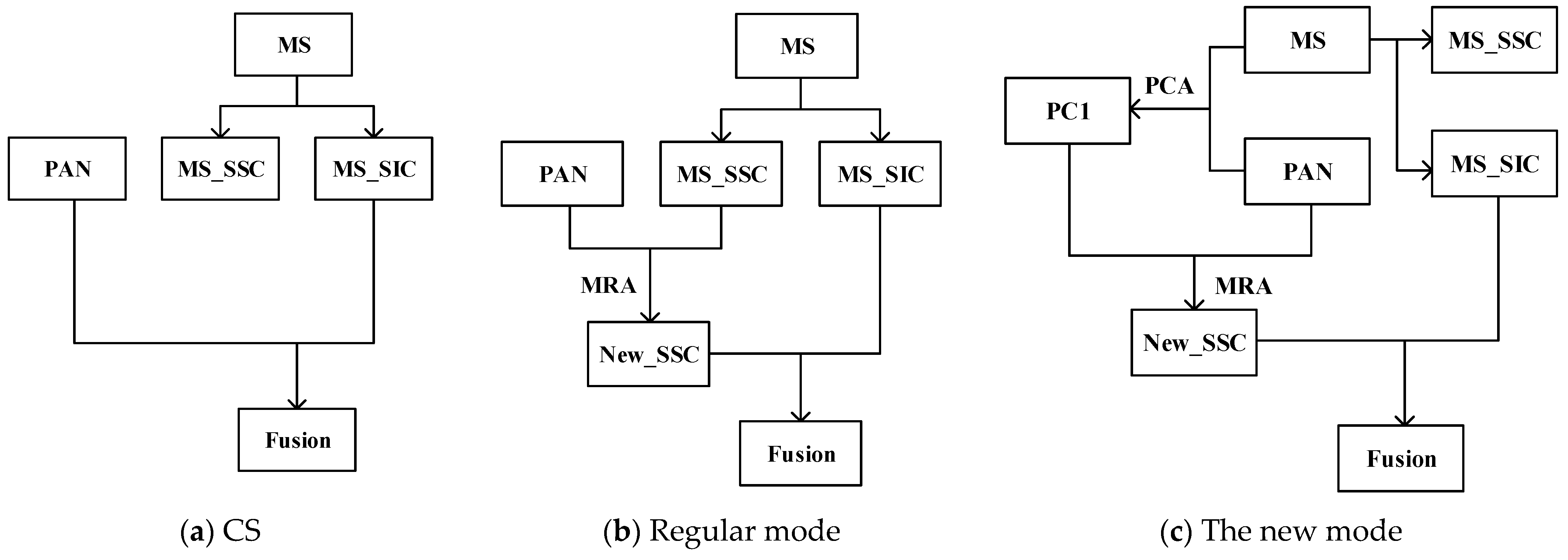
The CS approaches have good spatial quality but severe spectral distortion, while the MRA class methods have high spectral fidelity but poor spatial quality. These two types of method are complementary [11], which has given rise to many coupled methods. The conventional model of coupling method is shown in Figure 1a: (1) project MS into another vector space to separate the spectral information (MS_SIC) and spatial information (MS_SSC); (2) fuse MS_SSC and PAN using MRA-like methods to obtain the new spatial structure component (New-SSC); and (3) invert NEW-SSC and MS_SIC back to the original space to obtain the fused image. The addition of SSC reduces the information mismatch between PAN and MS, thus reducing the spectral distortion. However, the SSC is obtained directly from the MS, which lacks high-frequency spatial information, thus reducing the image’s sharpness. Although the coupling method can overcome the spectral distortion of CS and the spatial distortion of MRA, its spatial information quality (sharpness) is inferior to that of CS, and the spectral information quality (color) is inferior to that of MRA.

Therefore, it is of practical significance to optimize the coupling method to improve the quality of spatial information and the quality of spectral information of the fused images. The PCA technique can partially concentrate the spatial information shared by the bands in the first principal component through a linear transformation of the data. In this paper, a new fusion strategy is proposed, as shown in Figure 1b: (1) project MS into another vector space to separate the spectral information (MS_SIC) and spatial information (MS_SSC); (2) combine PAN and MS for PCA transformation and use the first principal component (PC1) as the spatial component (PC1_SSC); (3) use the MRA-like method to fuse PC1_SSC and PAN to obtain NEW-SSC; and (4) invert NEW-SSC and MS_SIC back to the original space to obtain the fused image. The difference between the new and conventional modes lies in how the spatial structure components are obtained: the conventional mode obtains the spatial structure components directly from MS using color space transformations and others. In contrast, using PCA transformation, the new mode obtains the spatial structure components from PAN and MS.

In the subsequent experiments, we selected the generalized intensity–hue–saturation (GIHS) algorithm from the CS methods and the NSST from the MRA class methods. In terms of fusion rules, this paper proposes a new low-frequency fusion rule using gradient-domain singular value decomposition (SVD) [12] and local structure descriptors to construct the weight coefficients, as well as a bootstrap filter [13], to guide the weights and to increase the spatial continuity of the weights; meanwhile, the high-frequency coefficients use local spatial frequencies to guide them.

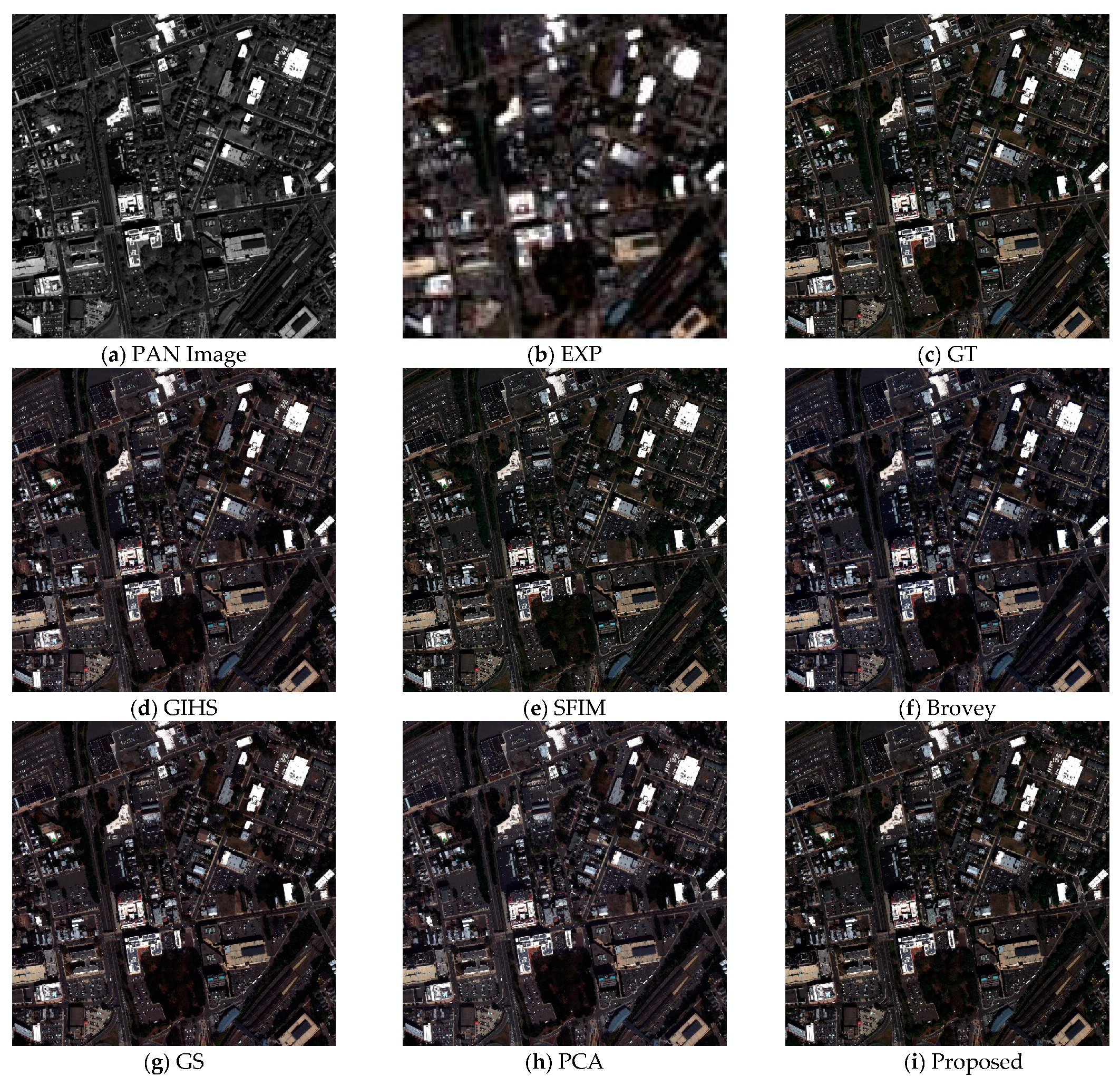
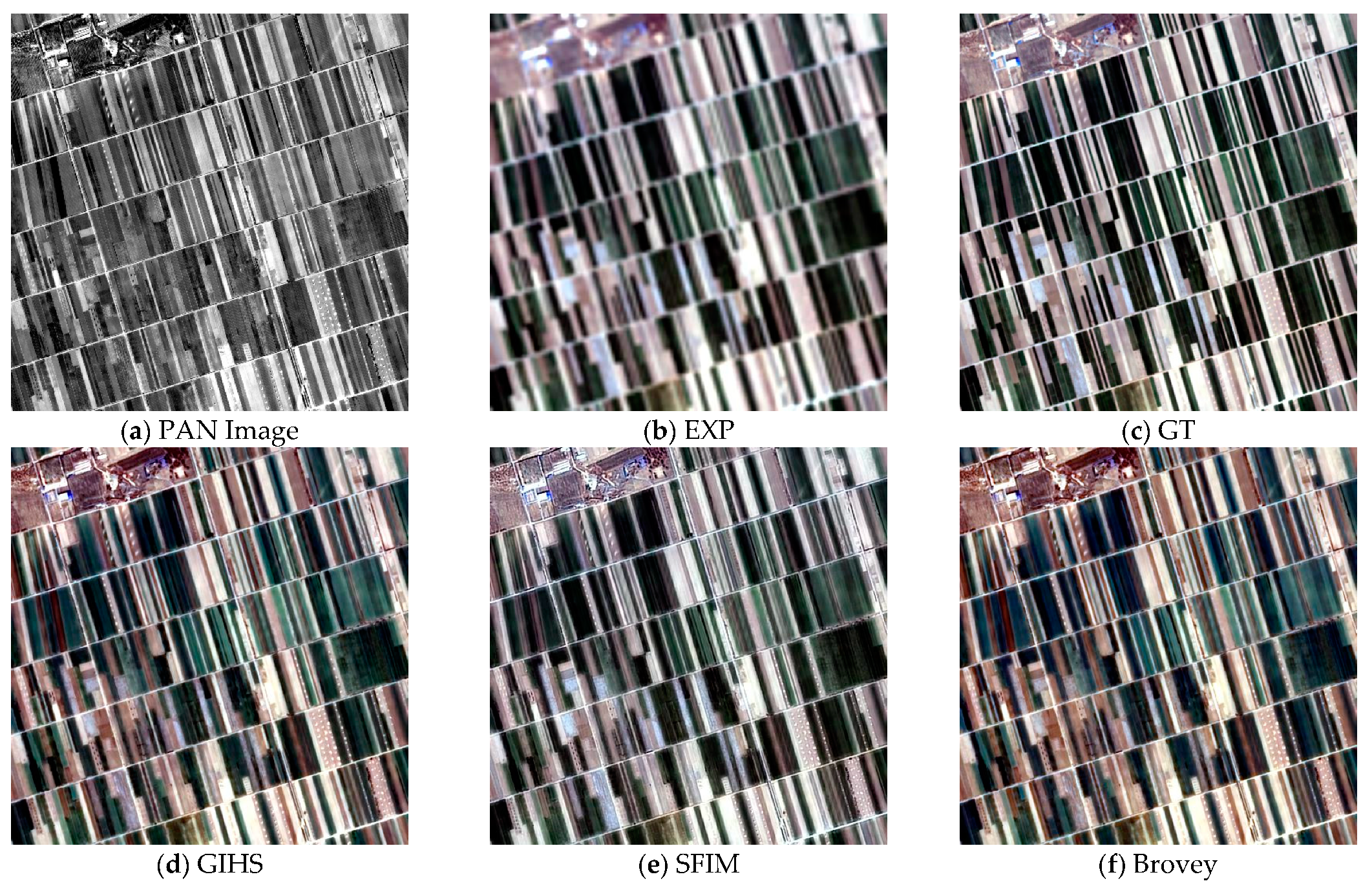
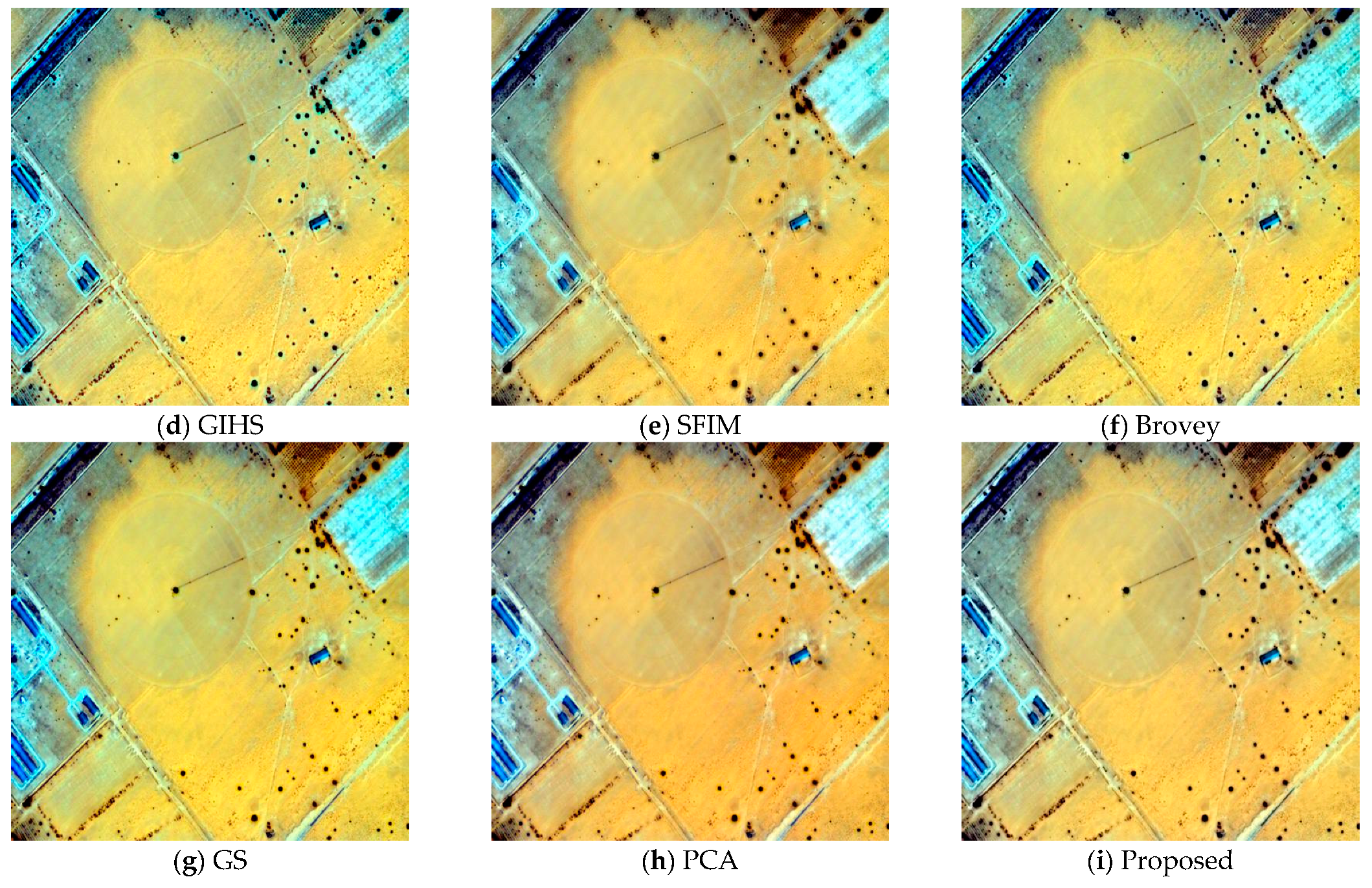
2. Methods

2.1. Overall Process

The GIHS [14,15] fusion algorithm is simple and efficient, with no limitation on the number of bands, and the NSST [16] has an excellent multi-scale decomposition capability and low computational complexity. Therefore, we utilize the GIHS as a CS algorithm and the NSST as an MRA algorithm in the novel coupling model shown in Figure 1c. Figure 2 specifically shows the algorithm flow, and Figure 3 is an expansion upon the subfigure within the solid red line of Figure 2 and shows the specific steps of the fusion of the component and PAN images. Both this paper’s method and GIHS essentially add detailed gain to the up-sampled MS image, while the difference lies in the source of the detailed gain. GIHS uses a difference map from PAN and multispectral intensity component I, as detailed gain. Additionally, this paper’s method first extracted principal component PC1 from PAN and MS using the PCA transform. Then, it used NSST to extract the new spatial structure component (New_SSC) from PC1 and PAN. Finally, the difference map of New_SSC and intensity component I were used as the detailed gain. This improvement meant that the New_SSC contained more detailed information from the MS and PAN images while retaining some spectral information, thus improving both the spatial and spectral accuracy of the final fused image. For the NSST in the framework, we propose a low-frequency coefficient fusion rule, based on a gradient-domain SVD and bootstrap filter (see Section 2.2 for details), and use the local spatial frequency reflecting the pixel neighborhood variation to fuse the high-frequency coefficients (see Section 2.3 for details). The specific steps are as follows:

(1)

Up-sample the MS image using three convolutional interpolations to obtain $M{S}^{*}$, making it the same size as the PAN image.

(2)

Combine intensity component I according to Equation (1), perform PCA transformation on the combination of $M{S}^{*}$ and PAN images, extract the first principal component PC1, and histogram match the PAN images and PC1 with I as the standard to obtain $PA{N}^{*}$ and $P{C}^{*}1$.

(3)

Perform NSST transform decomposition of $P{C}^{*}1$ and $PA{N}^{*}$ to obtain the low-frequency components ($L^{PC},L^{PAN})$ and the high-frequency component ($H_{j,k}^{PC},H_{j,k}^{PAN})$, respectively.

(4)

Fuse the low-frequency coefficients to obtain the new low-frequency components ($L^F),$ and fuse the high-frequency coefficients to obtain the new high-frequency component ($H_j^F,k)$.

(5)

The new low-frequency and high-frequency components are then NSST inverse transformed to obtain the primary fusion image ($F1$), and the GAIN will be obtained ($F1-I)$. Finally, use the f $Fi=Mi+\omega iGAIN$ formula to obtain the fusion image (F), where the detail modulation coefficient ($\omega$) is set to 1.

2.2. Low-Frequency Fusion Rules

The low-frequency coefficients include the primary information of the original images. Takeda [17] proposed an SVD of the image in the gradient domain. For image P, the steps of the gradient domain SVD are as follows:

(1) Calculate the gradients in the row and column directions of the image P.

(2) Form the local gradient values into an N × 2 matrix (G), with N referring to the number of local image elements.

(3) Perform singular value decomposition of G to obtain two singular values, λ1 and λ2.

$$G={\left[\nabla f1,\nabla f2\dots \nabla fN\right]}^T=US{V}^{*}$$

(1)

Here, $\nabla fi={\left[\nabla f_i^x,\nabla f_i^y\right]}^T$ refers to the gradient values of image P in the row and column directions at image element i. U is an N × N orthogonal matrix, S is an N × 2 matrix containing the singular values λ1 and λ2 on its diagonal, and V* is a 2 × 2 orthogonal matrix. The singular values λ1 and λ2 reflect the energy change of G in the eigenvector direction, and the magnitudes of λ1 and λ2 have different characteristics in the image-smoothing region, where the boundary is consistent with the texture direction and/or there is a more richly detailed region. Based on this, Ming Yin [16] proposed a new image structure descriptor based on $lsd\left(i\right)=\lambda 1\left(i\right)+\lambda 2\left(i\right)$ and demonstrated its ability to reflect the basic structural information of image localization. In this paper, a low-frequency coefficient fusion rule based on SVD and a bootstrap filter is proposed, as follows.

First, calculate the local structure descriptors $\left(L^{\mathit{PC}}{, L}^{\mathit{PAN}}\right)$ of the low-frequency component $({\mathit{lsd}}^{\mathit{PC}}{, \mathit{lsd}}^{\mathit{PAN}})$, and determine the initial weight matrices $weigh{t}^{PC}\mathrm{and} weigh{t}^{PAN}$ by comparing their sizes.

$$weigh{t}^{PC}\left(x,y\right)=\{\begin{array}{ll}1& ls{d}^{PC}\left(x,y\right)\ge ls{d}^{PAN}\left(x,y\right)\\ 0& ls{d}^{PC}\left(x,y\right)<ls{d}^{PAN}\left(x,y\right)\end{array},$$

(2)

$$weigh{t}^{PAN}\left(x,y\right)=1-weigh{t}^{PC}\left(x,y\right).$$

(3)

Process the weight matrix using bootstrap filtering to enhance its spatial continuity. Use $PC{1}^{*} \mathrm{and} PA{N}^{*}$ as bootstrap images, and apply bootstrap filtering $weigh{t}^{PC} \mathrm{and} weigh{t}^{PAN}$.

$$\begin{gathered} weigh{t}^{PC}=GF\left(weigh{t}^{PC},PC{1}^{*}\right) \\ weigh{t}^{PAN}=GF\left(weigh{t}^{PAN},PA{N}^{*}\right). \end{gathered}$$

(4)

The low-frequency coefficient fusion rule based on SVD and bootstrap filter can be written as:

$$L^F=weigh{t}^{PC}·L^{PC}+weigh{t}^{PAN}·L^{PAN}.$$

(5)

2.3. High-Frequency Fusion Rules

After NSST decomposition, each source image can be obtained as a series of high-frequency sub-band images. The high-frequency coefficients at different scales of NSST provide rich edge and texture information for the source images. The absolute values of the coefficients are larger when the edge and texture features are more pronounced [18]. Therefore, a considerable absolute value is usually used as the high-frequency coefficient selection rule. However, this rule ignores the correlation between neighboring pixels and may introduce noise into the fused image. The local spatial frequency (LSF) can reflect the pixel neighborhood activity index: the larger the LSF value, the more active the pixel points in the local region. Therefore, LSF is used to fuse high-frequency coefficients. The equation of LSF is as follows:

$$LSF\left(x,y\right)=\sqrt{LR{F}^2\left(x,y\right)+LC{F}^2\left(x,y\right)}.$$

(6)

where LRF and LCF denote the image’s local row frequency and column frequency, respectively, with the following equations:

$$\begin{gathered} LRF\left(x,y\right)= \\ \sqrt{\frac{1}{\left(2M+1\right)\left(2N+1\right)}{{\displaystyle \sum }}_{m=-M}^M{{\displaystyle \sum }}_{n=-N}^N{\left[H_{j,l}\left(x+m,y+m\right)-H_{j,l}\left(x+m,y+m-1\right)\right]}^2}, \end{gathered}$$

(7)

$$\begin{gathered} LCF\left(x,y\right)= \\ \sqrt{\frac{1}{\left(2M+1\right)\left(2N+1\right)}{{\displaystyle \sum }}_{m=-M}^M{{\displaystyle \sum }}_{n=-N}^N{\left[H_{j,l}\left(x+m,y+m\right)-H_{j,l}\left(x+m-1,y+m\right)\right]}^2}, \end{gathered}$$

(8)

where M and N represent the neighborhood size. Then, the SF-based HF coefficient selection rule can be written as:

$$H_{j,l}^F\left(x,y\right)=\left\{\begin{array}{c} H_{j,l}^{PC}\left(x,y\right) LS{F}_{j,l}^{PC}\left(x,y\right)\ge LS{F}_{j,l}^{PAN}\left(x,y\right)\\ H_{j,l}^{PAN}\left(x,y\right) LS{F}_{j,l}^{PC}\left(x,y\right)<LS{F}_{j,l}^{PAN}\left(x,y\right)\end{array}\right..$$

(9)

3. Evaluation Metrics

The purpose of fusion is to create a synthetic image that resembles reality. Ranchin [19] stated that the fused image should be as similar as possible to a high-resolution multispectral image obtained from the same sensor. In order to evaluate the performance of a certain method, there are two main techniques: one is the evaluation method with references, and the other is the evaluation method without references.

3.1. Evaluation Metrics with References

The evaluation model with references down-samples the original MS and PAN images using the cubic convolution method (the down-sampling factor is obtained based on the resolution ratio of the MS image to the PAN image), and the sampled images are fused. In this way, the original MS image is used as the reference image for assessing the image quality, and a method evaluation can be performed using the full reference method. The image quality assessment indexes used in this paper include the average gradient (AG), structural similarity (SSIM), correlation coefficient (CC), universal image quality indexes (UIQI) [20], spectral angle mapper (SAM) [21], and erreur relative global adimensionnelle de synthèse (ERGAS) [22], where AG can be used to measure the spatial quality of the fused image, and a larger value of AG indicates a clearer image; SSIM indicates the structural similarity between the two scenic images, and a higher SSI value indicates that the structure of the fused image is more similar to the reference image and that its spatial quality is better; the size of CC indicates the degree of correlation between the two images; UIQI is used to evaluate the degree of structural preservation of the image, and its optimal value is 1; SAM reflects the size of the spectral distortion between the reference image and the fused image, and a smaller value of SAM indicates a better spectral quality of the fused result; and ERGAS reflects the overall quality of the fused image, and a smaller value indicates a better quality of the fused image.

3.2. Evaluation Index without Reference

The evaluation mode without references fuses the original MS and PAN images directly. There is no actual reference image to evaluate the fusion results in this evaluation mode, so the method is evaluated using a comprehensive evaluation index without a reference. This method uses the spatial information of the PAN image to evaluate the spatial distortion index ($D_s$) of the fused image and the spectral information of the MS image to evaluate the spectral distortion index ($D_{\lambda }$) of the fusion influence, while the hybrid quality with no reference (HQNR) is calculated based on both images [23]. The smaller the values of $D_s$ and $D_{\lambda }$, the smaller the spatial and spectral distortion of the fused image, with the best value being 0. The larger the value of HQNR, the higher the overall evaluation of the fused image, with the best value being 0. This evaluation index can evaluate the performance of different fusion methods without references to real images.

4. Results

4.1. Experiment Preparation

In order to verify the reliability and generalizability of the method, fusion experiments were selected from four satellites with different feature types, as shown in the

Table 1. Experimental datasets.

Satellite	Spatial Resolution	Image Fast Size/Pixels	Feature Type
GE-1	0.46 m PAN, 1.84 m MS	2048 PAN, 512 MS	Urban
WV-4	0.31 m PAN, 1.24 m MS	2048 PAN, 512 MS	Plants and water
GF-7	0.8 m PAN, 3.2 m MS	2048 PAN, 512 MS	Farmland
GFDM	0.5 m PAN, 2 m MS	2048 PAN, 512 MS	Desert

. The four satellites were GeoEye-1 (GE-1), WorldView-4 (WV-4), Gaofen-7 (GF-7), and Gaofen Multi-Mode (GFDM), where the spatial resolutions of the PAN images were all at the sub-meter scale, between 0.31 and 0.8 m, and the spatial resolution of the MS images were at the meter scale, between 1.24 and 3.2 m. The feature types of the four scenes were urban, plants and water, agricultural land, and desert, covering some of the features that frequently appear during satellite observation of Earth. The PAN image block size was 2048 pixels, and the MS image fast size was 512 pixels. The GE-1 and WV-4 data were from the standard fusion dataset [24], GF-7 and GFDM were from the China Resource Satellite observation data, and each dataset was preprocessed using the exact alignment method [25,26].

In the subsequent experiments, for the experimental mode with references, the MS images were down-sampled to 128 × 128 pixels, the PAN images were down-sampled to 512 × 512 pixels, and the original MS images were used as the reference data. The experiments were performed with the original-sized data for the experimental mode without references, and the experimental effects of the different methods were evaluated using the method without references.

Five classic fusion algorithms were used as comparison methods: (1) GIHS fusion algorithm [14,27]; (2) SFIM fusion algorithm [27,28]; (3) Brovey fusion algorithm [14,28]; (4) GS fusion algorithm [13,27]; and (5) PCA fusion algorithm [27,29].

4.2. Experimental Results

4.2.1. Experimental Results with References

The test in this subsection was conducted using the model with references to compare the effects of different methods. Figure 4 shows the fusion images of GE-1 urban features. Figure 4a shows a down-sampled PAN image; Figure 4b shows an up-sampled image after the down-sampling of the MS image, which is noted as being an EXP (expanded) image; Figure 4c shows the original MS image, which was used as the reference image and is a GT (ground true) image; Figure 4d–i show the results under different fusion algorithms; and the subsequent experiments in this section were set up in this manner. It can be seen from the figure that different methods can successfully fuse PAN and MS images. However, the results of the GIHS, Brovey, and GS methods had some spectral distortion, while the spectra of the SIFM, GS, and this paper’s method were better maintained.

Furthermore, in terms of the details, the accuracy was better retained when using the method proposed in this paper. From the quantitative evaluation results in

Table 2. Objective assessment indexes of the GE-1 image fusion results.

	AG	SSIM	CC	UIQI	SAM	ERGAS
GT	59.1614	1.0000	1.0000	1.0000	0.0000	0.0000
EXP	17.2741	0.5551	0.8404	0.3548	6.7234	9.4465
GIHS	33.1363	0.8624	0.9592	0.7738	6.5338	5.9901
SFIM	32.7685	0.8470	0.9510	0.7577	6.1840	5.7623
Brovey	33.0581	0.8555	0.9593	0.7616	6.7234	6.1109
GS	33.0537	0.8630	0.9596	0.7744	6.4007	5.9720
PCA	32.9883	0.8578	0.9580	0.7700	6.4326	6.0185
Proposed	33.1592	0.8757	0.9559	0.7753	6.5093	5.6390

Bold indicates best results.

, it can also be seen that the AG and SSIM of this method were the highest among the various methods, indicating that this method had the best spatial detail retention, in addition to the best performance for the UIQI and ERGAS indexes, indicating its excellent spectral retention ability. The best performances for CC and SAM were found in the results of the GS and SFIM methods, respectively. However, on the whole, the best results were obtained by the method of this paper.

The fusion results for the WV-4 images with different algorithms are shown in Figure 5, and the scene mainly contains plants and water. It can be seen from the figure that the methods did not show any obvious color bias, but the sharpness of the SFIM method was significantly lower than the other methods. The clarity of the method presented in this paper was better than that of the other methods. The quantitative results in

Table 3. Objective assessment indexes of the WV-4 image fusion results.

	AG	SSIM	CC	UIQI	SAM	ERGAS
GT	19.4637	1.0000	1.0000	1.0000	0.0000	0.0000
EXP	6.7747	0.7495	0.9647	0.4070	46.5098	1.9421
GIHS	12.5299	0.9168	0.9845	0.7176	33.7666	2.2510
SFIM	11.5038	0.9169	0.9877	0.7100	30.3048	1.8093
Brovey	12.4041	0.9204	0.9855	0.7184	32.9954	1.9421
GS	12.2915	0.9308	0.9872	0.7311	32.1928	2.0890
PCA	12.2212	0.9089	0.9781	0.7120	39.3873	2.3635
Proposed	12.5323	0.9117	0.9882	0.7436	32.1953	2.1581

Bold indicates best results.

show that this method had the best performance for the AG value, while the SFIM method had the lowest AG value, which is also consistent with the visible results. Moreover, the method in this paper obtained the best performance for the CC and UIQI indexes. In contrast, the SFIM method obtained the best results for SAM and ERGAS, which indicates that the SFIM method had the best spectral retention ability on these data. However, on the whole, the method presented in this paper had the best results.

Figure 6 shows the fusion results of GF-7 images using different algorithms, and the scene is mainly farmland. For this scene’s images, the GIHS, Brovey, GS, and PCA methods showed a more obvious color bias, especially the GIHS and Brovey methods. The scene image is reddish with these two methods, while the GS and PCA methods are greenish. Conversely, the SFIM method and the method in this paper have an excellent overall spectrum. The quantitative evaluation results in

Table 4. Objective assessment indexes of the GF-7 image fusion results.

	AG	SSIM	CC	UIQI	SAM	ERGAS
GT	26.7046	1.0000	1.0000	1.0000	0.0000	0.0000
EXP	13.9148	0.7457	0.9262	0.5906	2.1305	1.7529
GIHS	21.3507	0.7901	0.9346	0.7120	2.1663	1.7281
SFIM	25.1842	0.8235	0.9444	0.7147	2.0730	1.4396
Brovey	21.6986	0.7861	0.9273	0.7061	2.1305	1.7403
GS	22.6489	0.7383	0.9035	0.6493	3.2087	2.0708
PCA	24.7823	0.5646	0.7376	0.4954	4.8963	3.1430
Proposed	21.5021	0.8312	0.9492	0.7149	2.0596	1.5690

Bold indicates best results.

show that the methods in this paper obtained the best results for the SSIM, CC, UIQI, and SAM indexes. At the same time, SFIM had the best results for the AG and ERGAS indexes, which is also consistent with the visual results.

Figure 7 shows the fusion results of the GFDM images using different algorithms, and the scene consists mainly of a desert. The figure shows that the color bias of the GIHS, Brovey, and GS methods is serious, while the color bias of the PCA method is better for the desert scene. Furthermore, the results of the SFIM and this paper’s method are relatively good. In addition, the sharpness of this paper’s method is significantly higher than the other methods. This can also be verified from the quantitative evaluation results in

Table 5. Objective assessment indexes of the GFDM image fusion results.

	AG	SSIM	CC	UIQI	SAM	ERGAS
GT	9.9422	1.0000	1.0000	1.0000	0.0000	0.0000
EXP	3.2438	0.7664	0.9287	0.4348	0.1639	0.2926
GIHS	7.6976	0.8795	0.9487	0.6824	0.2107	0.2290
SFIM	7.8605	0.8993	0.9719	0.6956	0.1554	0.1755
Brovey	7.6017	0.8952	0.9602	0.7043	0.1639	0.2078
GS	7.7288	0.8876	0.9632	0.6821	0.1978	0.2171
PCA	7.8874	0.8890	0.9623	0.6784	0.2139	0.2008
Proposed	7.9766	0.9004	0.9503	0.6841	0.2103	0.2244

Bold indicates best results.

. The AG and SSIM indexes of this paper’s method demonstrate that it had the best performance, while SFIM obtained better results for CC, SAM, and ERGAS, indicating its better spectral retention ability.

4.2.2. Experimental Results without References

In order to further verify the effectiveness of the method in this paper, reference-free metrics were used to evaluate the real fusion images, and the data and methods involved in the validation were consistent with those in the previous subsection, although there was no real GT reference data for the validation in this experiment.

Table 6. Objective assessment indexes of fusion results without references.

Satellite	Index	EXP	GIHS	SFIM	Brovey	GS	PCA	Proposed
GE-1	$D_{\lambda }$	0.0685	0.1090	0.1429	0.1055	0.1064	0.1259	0.0927
	$D_s$	0.1516	0.0298	0.0178	0.0297	0.0298	0.0196	0.0065
	$HQNR$	0.7901	0.8643	0.8417	0.8678	0.8668	0.8568	0.9012
WV-4	$D_{\lambda }$	0.1014	0.2130	0.1123	0.2006	0.1977	0.2737	0.0806
	$D_s$	0.2714	0.1123	0.1411	0.1123	0.1123	0.0923	0.0855
	$HQNR$	0.6545	0.6985	0.7623	0.7094	0.7120	0.6592	0.8406
GF-7	$D_{\lambda }$	0.0086	0.1114	0.0225	0.1082	0.1273	0.2889	0.0153
	$D_s$	0.2004	0.0375	0.0751	0.0375	0.0375	0.0103	0.0705
	$HQNR$	0.7926	0.8552	0.9040	0.8582	0.8398	0.7036	0.9152
GFDM	$D_{\lambda }$	0.0426	0.2020	0.0271	0.1876	0.0312	0.1354	0.0459
	$D_s$	0.0694	0.0312	0.0253	0.0312	0.1372	0.0253	0.0197
	$HQNR$	0.8908	0.7729	0.9482	0.7869	0.8357	0.8425	0.9351

Bold indicates best results.

shows the evaluation results without a reference index for the different methods. The method presented in this paper obtained relatively better results for four different satellites and four scenes, and the spatial aberration index $D_s$ was the best in these four scenes. The comprehensive evaluation index HQNR and spatial aberration index were the best for GE-1, WV-4, and GF-7. In addition, the spectral aberration index had the best performance for these images.

In summary, the method in this paper achieved better results for four different scenes of the GE-1, WV-4, GF-7, and GFDM satellites (urban, plants and water, farmland, and desert) compared with the other methods, which shows that the method presented in this paper has good universality and generality.

5. Discussion

As demonstrated by the previous experimental results, the proposed method achieved good results for both the evaluation system with references and the evaluation system without references and was obviously better than the comparison methods, especially in the index test on the retention of spatial structure information. The conventional mode of extracting spatial structure information through conventional spectral methods and spatial methods mainly uses color space transformation and other techniques to obtain spatial structure components from images. In contrast, the method proposed in this paper uses PCA transformation to jointly extract spatial structure components from PAN and MS images, which can better preserve and fuse the obtained spatial information. The above experiments also verified this point of view. Compared with the conventional method, it can be seen that the method in this paper retained more spatial details. Compared with a single spectral method and a spatial method, the method given in this paper combines the advantages of the two. The optimized coupling method used in this paper can improve the quality of the spatial information and spectral information of the fused image. In this paper, PCA technology was used to concentrate the part of the spatial information shared by the bands in the first principal component; to obtain the spatial components through linear transformation of the data; to make full use of the acquired spatial information of all the bands; and, on this basis, to extract the MS image. The spectral information is fused with this to obtain the final fused image. However, the method given in this paper uses PCA transformation when extracting spatial structure information. Although this transformation can concentrate the main information in the first component, it will inevitably lose part of the spatial structure information. In the future, we could study how to use deep learning to extract spatial structure information from the original image and then inject this into the low-frequency spectral component to avoid interference by human factors.

6. Conclusions

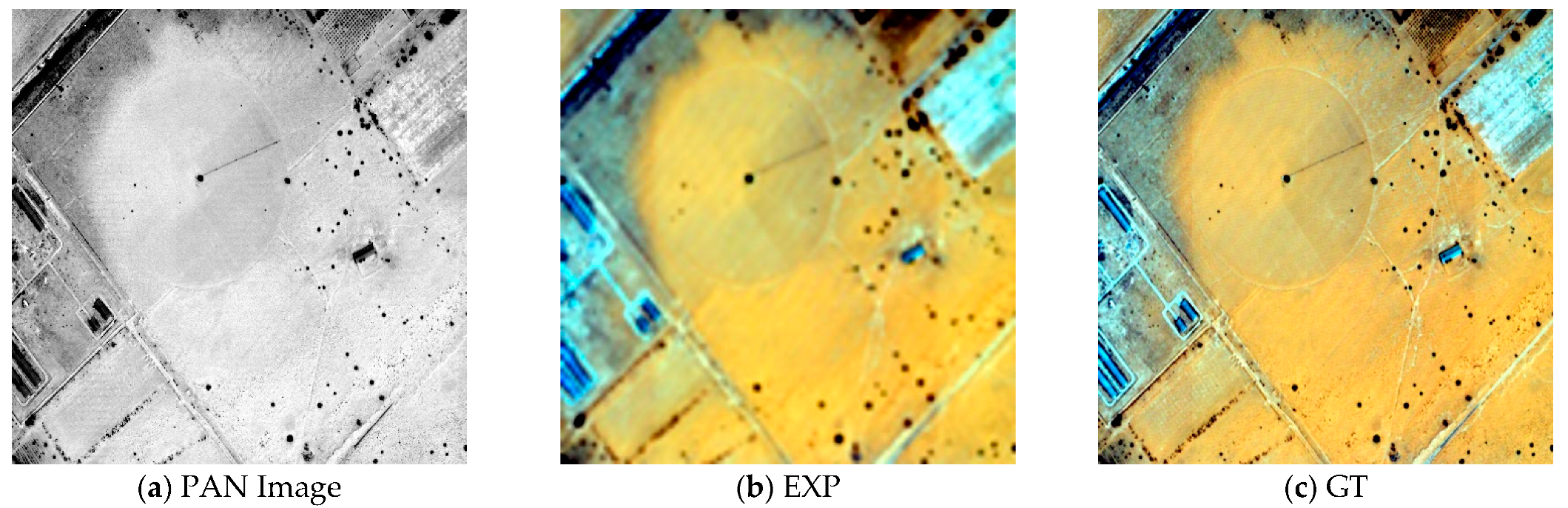
For the fusion of PAN and MS images, a fusion framework combining GIHS, NSST, and PCA was proposed in this paper. The GIHS method was improved to take advantage of its concise formulas and high execution efficiency, while there was no limitation on the number of bands of input data. The constructed fusion algorithm contains more spatial structure information of MS and PAN images and retains some spectral information of MS. PCA is applied to each band of the PAN image and MS image to obtain the first principal component, and then NSST decomposition is used in the fusion with the PAN image. Finally, the fused image is used to replace the original intensity component, which can enhance the fusion effect and reduce the spectral distortion. Compared with the traditional algorithms, the algorithm in this paper obtained more spatial structure components from PAN and MS and could preserve spectral information with high fidelity while effectively retaining spatial structure information. In the process of low-frequency coefficient fusion, this paper proposed a new fusion rule based on the gradient-domain SVD, using a local structure description operator to obtain the initial fusion weights and bootstrap filtering to increase the spatial continuity of these weights. Four scenes of urban, plants and water, farmland, and desert images from GeoEye-1, WorldView-4, Gaofen-7, and GFDM were used as experimental data for a fusion method study. The method was compared with five other fusion algorithms, using the average gradient, structural similarity, correlation coefficient, common image quality index, spectral angle mapping, and relative global error, with and without evaluation indexes, including the spectral aberration index, spectral distortion index, and comprehensive evaluation index in the reference mode. The results showed that the method proposed in this paper achieved outstanding results in spectral preservation and spatial information incorporation.

References

1. Wang, M.; He, L.; Cheng, Y.; Chang, X. Panchromatic and Multi-spectral Fusion Method Combined with Adaptive Gaussian Filter and SFIM Model. Acta Geod. Cartogr. Sin. 2018, 47, 82–90. [Google Scholar]
2. Kang, X.; Li, S.; Benediktsson, J.A. Pansharpening With Matting Model. IEEE Trans. Geosci. Remote Sens. 2014, 52, 5088–5099. [Google Scholar] [CrossRef]
3. Xing, Y.; Zhang, Y.; Yang, S.; Zhang, Y. Hyperspectral and multispectral image fusion via variational tensor subspace decomposition. IEEE Geosci. Remote Sens. Lett. 2021, 19, 5001805. [Google Scholar] [CrossRef]
4. Xing, Y.; Yang, S.; Feng, Z.; Jiao, L. Dual-collaborative fusion model for multispectral and panchromatic image fusion. IEEE Trans. Geosci. Remote Sens. 2020, 60, 5400215. [Google Scholar] [CrossRef]
5. Aiazzi, B.; Alparone, L.; Baronti, S.; Garzelli, A. Context-driven fusion of high spatial and spectral resolution images based on oversampled multiresolution analysis. IEEE Trans. Geosci. Remote Sens. 2002, 40, 2300–2312. [Google Scholar] [CrossRef]
6. Candes, E.J.; Donoho, D.L. Recovering edges in ill-posed inverse problems: Optimality of curvelet frames. Ann. Stat. 2002, 30, 784–842. [Google Scholar] [CrossRef]
7. Do, M.N.; Vetterli, M. The contourlet transform: An efficient directional multiresolution image representation. IEEE Trans. Image Process. 2005, 14, 2091–2106. [Google Scholar] [CrossRef] [Green Version]
8. Da Cunha, A.L.; Zhou, J.; Do, M.N. The nonsubsampled contourlet transform: Theory, design, and applications. IEEE Trans. Image Process. 2006, 15, 3089–3101. [Google Scholar] [CrossRef] [Green Version]
9. Gao, Y.; Jia, Z.; Qin, P.; Wang, L. Medical Image Fusion Based on Compressive Sensing and Adaptive PCNN. Comput. Eng. 2018, 44, 224–229. [Google Scholar]
10. Kong, L.; Zhang, Z.; Zeng, X.; Wang, Q. Infrared and Visible Image Fusion Algorithm Based on NSST and SWT. Packag. Eng. 2018, 39, 216–222. [Google Scholar]
11. Ghassemian, H. A review of remote sensing image fusion methods. Inf. Fusion 2016, 32, 75–89. [Google Scholar] [CrossRef]
12. He, K.; Sun, J.; Tang, X. Guided Image Filtering. In European Conference on Computer Vision 2010; Springer: Berlin/Heidelberg, Germany, 2010. [Google Scholar]
13. Aiazzi, B.; Baronti, S.; Selva, M. Improving component substitution pansharpening through multivariate regression of MS + Pan data. IEEE Trans. Geosci. Remote Sens. 2007, 45, 3230–3239. [Google Scholar] [CrossRef]
14. Tu, T.M.; Su, S.C.; Shyu, H.C.; Huang, P.S. A new look at IHS-like image fusion methods. Inf. Fusion 2001, 2, 177–186. [Google Scholar] [CrossRef]
15. Easley, G.; Labate, D.; Lim, W.Q. Sparse directional image representations using the discrete shearlet transform. Appl. Comput. Harmon. Anal. 2008, 25, 25–46. [Google Scholar] [CrossRef] [Green Version]
16. Yin, M.; Liu, W.; Zhao, X.; Yin, Y.; Guo, Y. A novel image fusion algorithm based on nonsubsampled shearlet transform. Optik 2014, 125, 2274–2282. [Google Scholar] [CrossRef]
17. Takeda, H.; Farsiu, S.; Milanfar, P. Kernel regression for image processing and reconstruction. IEEE Trans. Image Process. 2007, 16, 349–366. [Google Scholar] [CrossRef] [Green Version]
18. Deng, L.; Yao, X. Research on the Fusion Algorithm of Infrared and Visible Images Based on Non-subsampled Shearlet Transform. Acta Electron. Sin. 2017, 45, 2965–2970. [Google Scholar]
19. Ranchin, T.; Wald, L. Fusion of high spatial and spectral resolution images: The ARSIS concept and its implementation. Photogramm. Eng. Remote Sens. 2000, 66, 49–61. [Google Scholar]
20. Wang, Z.; Bovik, A.C. A universal image quality index. IEEE Signal Process. Lett. 2002, 9, 81–84. [Google Scholar] [CrossRef]
21. De Carvalho, O.A.; Meneses, P.R. Spectral correlation mapper (SCM): An improvement on the spectral angle mapper (SAM). In Summaries of the 9th JPL Airborne Earth Science Workshop; JPL Publication: Pasadena, CA, USA, 2000. [Google Scholar]
22. Wald, L. Quality of high resolution synthesised images: Is there a simple criterion? In Proceedings of the Third Conference Fusion of Earth data: Merging Point Measurements, Raster Maps and Remotely Sensed Images, Sophia Antipolis, France, 26–28 January 2000; pp. 99–103. [Google Scholar]
23. Vivone, G.; Mura, M.D.; Garzelli, A.; Restaino, R.; Scarpa, G.; Ulfarsson, M.O.; Alparone, L.; Chanussot, J. A new benchmark based on recent advances in multispectral pansharpening: Revisiting pansharpening with classical and emerging pansharpening methods. IEEE Geosci. Remote Sens. Mag. 2020, 9, 53–81. [Google Scholar] [CrossRef]
24. Vivone, G.; Dalla Mura, M.; Garzelli, A.; Pacifici, F. A benchmarking protocol for pansharpening: Dataset, preprocessing, and quality assessment. IEEE J. Sel. Top. Appl. Earth Obs. Remote Sens. 2021, 14, 6102–6118. [Google Scholar] [CrossRef]
25. Xie, G.; Wang, M.; Zhang, Z.; Xiang, S.; He, L. Near real-time automatic sub-pixel registration of panchromatic and multispectral images for pan-sharpening. Remote Sens. 2021, 13, 3674. [Google Scholar] [CrossRef]
26. Wang, M.; Xie, G.; Zhang, Z.; Wang, Y.; Xiang, S.; Pi, Y. Smoothing Filter-Based Panchromatic Spectral Decomposition for Multispectral and Hyperspectral Image Pansharpening. IEEE J. Sel. Top. Appl. Earth Obs. Remote Sens. 2022, 15, 3612–3625. [Google Scholar] [CrossRef]
27. Vivone, G.; Alparone, L.; Chanussot, J.; Mura, M.D.; Garzelli, A.; Licciardi, G.A.; Restaino, R.; Wald, L. A critical comparison among pansharpening algorithms. IEEE Trans. Geosci. Remote Sens. 2015, 53, 2565–2586. [Google Scholar] [CrossRef]
28. Liu, J.G. Smoothing filter-based intensity modulation: A spectral preserve image fusion technique for improving spatial details. Int. J. Remote Sens. 2000, 21, 3461–3472. [Google Scholar] [CrossRef]
29. Kwarteng, P.; Chavez, A. Extracting spectral contrast in Landsat Thematic Mapper image data using selective principal component analysis. Photogramm. Eng. Remote Sens. 1989, 55, 339–348. [Google Scholar]
Figure 1. Hybrid model of the CS method and MRA method.
Applsci 13 01412 g001
Figure 2. Flowchart of the proposed method.
Applsci 13 01412 g002
Figure 3. Fusion flowchart of PC1 and the PAN image using the NSST transform.
Applsci 13 01412 g003
Figure 4. Fusion results for GE-1 images using different methods.
Applsci 13 01412 g004
Figure 5. Fusion results for the WV-4 images using different methods.
Applsci 13 01412 g005
Figure 6. Fusion results for the GF-7 images using different methods.
Applsci 13 01412 g006aApplsci 13 01412 g006b
Figure 7. Fusion results for the GFDM images using different methods.
Applsci 13 01412 g007aApplsci 13 01412 g007b