Article

Vehicle Trajectory Prediction Based on Graph Convolutional Networks in Connected Vehicle Environment

1
School of Mechanical Engineering, Beijing Institute of Technology, Beijing 100081, China
2
School of Vehicle and Energy, Yanshan University, Qinhuangdao 066004, China
*
Author to whom correspondence should be addressed.
Appl. Sci. 2023, 13(24), 13192; https://doi.org/10.3390/app132413192
Submission received: 8 November 2023 / Revised: 5 December 2023 / Accepted: 6 December 2023 / Published: 12 December 2023

Abstract

:
Vehicle trajectory prediction is an important research basis for the decision making and path planning of the intelligent and connected vehicle. In the connected vehicle environment, vehicles share information and drive cooperatively, and the intelligent and connected vehicles are able to obtain more accurate and rich perception information, which provides a data basis for accurate prediction of vehicle trajectories. However, attaining accurate and effective vehicle trajectory predictions poses technical challenges due to insufficient extraction of vehicular spatial–temporal interaction features. In this paper, we propose a vehicle trajectory prediction model based on graph convolutional neural network (GCN) in a connected vehicle environment. Specifically, using the driving scene information obtained by the intelligent and connected vehicle, the spatial graph and temporal graph are constructed based on the spatial interaction coefficient (SIC) and self-attention mechanism, respectively. Then, the graph data are entered into the interaction extraction module, and the spatial interaction features and temporal interaction features are extracted separately using the graph convolutional networks, which are fused to obtain the spatial–temporal interaction information. Finally, the interaction features are learned based on the convolutional neural networks to output the future trajectory information of all vehicles in the scene by one forward operation rather than a step-by-step process. The ablation experiment results show that the method proposed in this study to model the spatiotemporal interaction among vehicles based on SIC and self-attention mechanism reduces the prediction error by 5% and 12%, respectively. The results from the model comparison experiment show that the proposed method engenders an 8% improvement in prediction accuracy over the state-of-the-art solution, providing technical and theoretical support for trajectory prediction research of intelligent and connected vehicles.

1. Introduction

Intelligent and connected vehicles (ICVs) are equipped with cameras, lidar, and other on-board sensors as well as controllers, actuators, and other devices, integrating modern network communication technology which can fulfil the functions of environment perception, intelligent decision making, and cooperative control [1]. As the bridge between environment perception and decision making, the accuracy and rationality of trajectory prediction results directly affect the rationality and safety of subsequent decision making and path planning of ICVs. However, due to the complex interactions among vehicles, the generation of accurate and efficient predictions with respect to the vehicle trajectories in the future has become a recognized problem and challenge in both academia and industry.
In response to the above problem, researchers have conducted in-depth studies, and the existing vehicle trajectory prediction methods can be roughly grouped into four categories [2]: (1) physics-based methods; (2) classic machine-learning-based methods; (3) deep-learning-based methods; (4) reinforcement-learning-based methods. However, the physics-based vehicle trajectory prediction methods [3,4] are only applicable to short-term trajectory predictions with a prediction horizon of no more than 1s, and cannot effectively complete the medium- and long-term prediction tasks; classic machine-learning-based methods [5,6], on the other hand, are mostly only applicable to simpler driving scenes, and have poor trajectory prediction effects in complex driving scenes. Reinforcement-learning-based methods [7,8] require higher computational and time costs compared to other prediction methods.
Vehicle trajectory prediction methods based on deep learning consider not only physics-related factors but also interaction-related factors and are able to adapt to more complex traffic scenes. Thus, deep-learning-based [9,10,11,12] vehicle trajectory prediction methods have been gaining popularity in recent years. Early prediction models based on recurrent neural networks (RNNs) only use a single RNN module, as available literature [13] uses a module based on a three-layer long short-term memory (LSTM) stack to extract feature information for the prediction of the future trajectory of the vehicle. Subsequent scholars have mostly used multiple RNN modules with different functions. For example, the first LSTM-based module in the literature [14] was used to identify driving intentions, which were then fed into the second LSTM-based module along with vehicle longitudinal feature parameters for trajectory prediction. Inspired by the great success of convolutional neural networks (CNNs) in the field of computer vision in recent years, researchers have tried to apply CNNs to the field of vehicle trajectory prediction. CS-LSTM [15] introduces convolutional layers to replace the fully connected layers in the Social-LSTM network [16] to extract the vehicle spatial interaction information stored in the social tensor, which further improves the accuracy of prediction. The MANTRA algorithm [17] uses CNN-based memory enhancement networks to process historical trajectories and semantic map information to understand and learn scene pictures and scene features. The emergence of transformers (TFs) [18] has encouraged scholars to focus on attention mechanisms (AMs). The ST-attention module [19] introduces the AM into the prediction network to extract temporal affinity, i.e., the importance weights of historical trajectory information at different moments. Available literature [20] extracts vehicle and road information based on multi-head attention to output the probability distribution of future vehicle trajectories.
Although the abovementioned vehicle trajectory prediction methods based on RNN, CNN, and AM have achieved good prediction accuracy and promoted the development of the field of vehicle trajectory prediction to a certain extent, most of them extract the spatial interaction features among vehicles based on Euclidean data, while, in fact, the spatial interaction relations among vehicles are non-Euclidean [21]; this leads to the above methods having important limitations. As an efficient method to process non-Euclidean data, graph neural networks (GNNs) can avoid this problem by applying the algorithmic principle. The GRIP model [22] converts the raw vehicle data into graph data and then extracts the spatial–temporal interaction features in the graph data based on the convolution operation, further improving the accuracy of vehicle trajectory prediction. A further example is afforded by the GSTCN algorithm [21], which uses the reciprocal of the distance between two vehicles to construct the weighted adjacency matrix based on prior knowledge, and then learns the spatial–temporal interaction relations among vehicles based on graph convolutional networks (GCNs).
However, GNN-based prediction methods still have the problem of inadequate spatial–temporal interaction modeling. Specifically, most of these methods only construct spatial graphs based on the raw vehicle position coordinate data, without making full use of other parameters of the vehicle. Moreover, they model temporal dependencies based on the extracted spatial interaction information which, to some extent, destroys the original temporal interaction structure and eventually leads to inadequate extraction of spatial–temporal interaction relations.
To solve the above problems, this paper proposes a new trajectory prediction model called VTP-GCN. First, we comprehensively consider the historical coordinates and vehicle movement velocity information of the vehicles, propose the concept of spatial interaction coefficient (SIC) to characterize the intensity of spatial interaction between two vehicles, and optimize the weighted adjacency matrix of the existing spatial graph based on this coefficient. Meanwhile, to ensure the integrity of the temporal interaction structure entered into the temporal interaction extraction module, we construct a temporal graph based on the vehicle historical parameters rather than the extracted intra-spatial interaction features and utilize the self-attention mechanism to automatically capture and learn the interaction weights in the temporal weighted adjacency matrix. The interaction features hidden in the spatial and temporal graphs are extracted separately using GCN and then the two are fused to obtain the spatial–temporal interaction features of vehicles in the driving scene. In the trajectory prediction module, the spatial–temporal interaction features are used as input based on a fully convolutional operation to generate the trajectory positions of the vehicles in the next 5 s with only one forward step needed.
The main contributions of our work are as follows.
  • A new vehicle trajectory prediction framework, VTP-GCN, is proposed to model the spatial–temporal interaction behavior and output the future motion trajectories of vehicles based on GCN and fully convolutional layers, with the data from the comparative experiments showing that this method is effective in improving the accuracy of vehicle trajectory prediction.
  • The concept of spatial interaction coefficient is proposed to mark the intensity of spatial interaction between two vehicles, with the results from the ablation test showing that the weighted adjacency matrix based on the spatial interaction coefficient can better model the spatial interaction behavior among vehicles and the corresponding model has a better prediction performance.
  • A temporal graph construction method based on the self-attention mechanism is proposed to model the temporal interaction of vehicles at different historical moments, with the ablation test results showing that the relevant model is associated with smaller prediction errors than those associated with the reciprocal of the time interval.
The rest of this paper is arranged as follows. Section 2 describes the research problem object of this paper. Section 3 introduces the VTP-GCN model in detail. Section 4 presents the experiment results and discusses the trajectory prediction effect of VTP-GCN. Section 5 concludes this paper.

2. Problem Description

Reasonable and accurate trajectory prediction results can help ICVs understand the current driving scene, perceive driving risks in advance, and then make effective decisions and plans. In this paper, we assumed that the position coordinates and velocity information of vehicles in the scene had been obtained through the networked environment. We denote the feature information X of vehicles in the scene over a past time horizon th as:
X = [ P 1 , P 2 , , P t h ]
P t = [ ( x t 1 , y t 1 , v t 1 ) , ( x t 2 , y t 2 , v t 2 ) , , ( x t N , y t N , v t N ) ]
where Pt is the feature information of all vehicles in the scene at the time t, N is the number of vehicles in the scene, x and y are the position coordinates of the vehicle, and v is the velocity of the vehicle. We denote the predicted trajectories in the future time horizon tf as:
Y = [ P ^ t h + 1 , P ^ t h + 2 , , P ^ t h + t f ]
where,
P ^ t h + t = [ ( x ^ t h + t 1 , y ^ t h + t 1 ) , ( x ^ t h + t 2 , y ^ t h + t 2 ) , , ( x ^ t h + t N , y ^ t h + t N ) ]
are the predicted vehicles coordinates at the time th + t’.
Therefore, the vehicle trajectory prediction in this paper can be summarized as: enter the historical feature information X into the prediction model and hope that the model can generate the future position coordinates Y of the vehicles in the scene.

3. The VTP-GCN Model

The overall framework of the trajectory prediction model proposed in this paper is shown in Figure 1 and mainly includes three parts: the spatial graph and time graph representation module based on the raw vehicle data, the spatial–temporal interaction feature extraction module based on GCN, and the trajectory prediction module based on the fully convolutional operations.

3.1. Graph Representation Based on Raw Vehicle Motion Data

The complex spatial and temporal dependencies among vehicles in driving scenes are crucial to vehicle trajectory prediction. In order to effectively extract the vehicle spatial–temporal interaction information existing in the historical vehicle data, this paper presents the raw data as X i n _ s N × C × t h and X i n _ t t h × C × N , respectively, where N represents the number of the vehicles in the driving scene, and C = 3 represents the number of features (coordinates and velocity). Then, X i n _ s and X i n _ t are entered into the spatial graph representation module and the temporal graph representation module, respectively.
(1)
Spatial Graph Representation Learning
The spatial graph is defined as a sparse undirected graph G s p a = { G s p a _ t | t { 1 , 2 , , t h } } , where G s p a _ t represents the spatial interactions of vehicles at the time t . Supposing that there are N vehicles in the driving scene, we define G s p a _ t as G s p a _ t = { V s p a _ t , E s p a _ t } , where V s p a _ t = { υ t i | i { 1 , 2 , , N } } is the set of vehicles in the scene, and the coordinates ( x , y ) are the attribute of every vertex representing a vehicle. Meanwhile, E s p a _ t = { e t i j | i , j { 1 , 2 , , N } } is the set of all edges which indicate whether two vertices are connected, that is, whether there is a spatial interaction between the two vehicles, with e t i j = 1 if the interaction is present, e t i j = 0   if the interaction is not present. The spatial interaction range of the two vehicles is shown by the blue dotted line in Figure 2. In this research, the spatial interaction range is limited to ± L m in the longitudinal direction and two adjacent lanes in the lateral direction. The gray vehicles in Figure 2 indicate the predicted vehicles, the yellow vehicles indicate the neighbor vehicles that interact spatially with the predicted vehicles, and the green vehicles indicate the unrelated vehicles that do not interact spatially with the predicted vehicles.
In previous research on vehicle trajectory prediction based on graph neural networks, in order to simplify calculations, researchers have assumed that each edge has the same weight when constructing the spatial graph, that is, the intensity of spatial interactions between the vehicle and its neighboring vehicles are the same. However, this assumption completely violates the natural driving situation, and the different motion states of different neighboring vehicles have completely different effects on the vehicle. For example, when a vehicle is driving on a lane at a certain speed, a neighboring vehicle located 10 m ahead will interact more strongly with said vehicle than a neighboring vehicle 60 m ahead. At the same time, neighboring vehicles that are separated from the vehicle in question by the same distance but travel at different velocities will also have different effects on the vehicle. Therefore, to mark the intensity of spatial interactions among vehicles, we propose the concept of spatial interaction coefficient (SIC). Its numerical value is inversely proportional to the Euclidean distance between two vehicles and directly proportional to the velocity difference, something which is in line with people’s conventional cognition. Subsequent ablation experiments have proven that constructing the spatial interaction graph based on the SIC can help improve the accuracy of vehicle trajectory prediction. We will elaborate on the specific content in Section 4.4. SIC is calculated with the following formula:
S I C i j = { | v i v j | D i j ,   i j   and   d i j L 0         ,   Otherwise
where v i is the velocity of vehicle i , D i j is the Euclidean distance between vehicle i and vehicle j , and d i j is the longitudinal distance between the two vehicles. Based on the SIC, we constructed a weighted adjacency matrix A s p a _ t N × N to represent the spatial interdependencies of all vehicles in the scene. Thus, A s p a _ t can be obtained by the following equation:
A s p a _ t = ( 0 S I C 1 , 2 S I C 1 , 3 S I C 1 , N S I C 2 , 1 0 S I C 2 , 3 S I C 2 , N S I C 3 , 1 S I C 3 , 2 0 S I C 3 , N S I C N , 1 S I C N , 2 S I C N , 3 0 )
We can obtain the adjacency matrix A s p a N × N × t h of the spatial graph G s by stacking A s p a _ t at each historical time moment, and obtain the vertex feature matrix V s p a t h × N × C g of the spatial graph G s by stacking the V s p a _ t , where C g = 2 represents the position coordinates ( x , y ) .
(2)
Temporal Graph Representation Learning
Most of the existing studies on GCN-based vehicle trajectory prediction [21,22] use a single spatial graph to extract spatial and temporal interaction features successively, and this method based on the extracted spatial interaction information may lead to insufficient extraction of temporal interaction features. To overcome this problem, we propose the construction of the temporal graph based on the raw vehicle data to extract the interaction relations of vehicles at different historical time instants and, successively, its fusion with the spatial interaction feature to obtain the spatial–temporal interaction feature. Since the historical state of the vehicle can affect its future trajectory, and the future trajectory cannot affect the past historical state of the vehicle, we define the temporal graph as a spare directed graph G t m p = { G t m p _ i | i { 1 , 2 , , N } } , where G t m p _ i = { V t m p _ i , E t m p _ i } represents the temporal graph of the ith vehicle, and V t m p _ i = { υ t i | t 1 , 2 , t h } is the set of all historical time instants. E t m p _ i = { e k q i | k , q { 1 , 2 , , t h } } is the set of all temporal edges, where e k q i = 1 if v k i is connected to v q i , that is, the time instant k < q , and e k q i = 0 if v k i is not connected to v q i .
The movement status of a vehicle at different historical moments has different impacts on its future movement trajectory. How to accurately mark this temporal interaction intensity is crucial to generate accurate predictions of vehicle trajectories. With the proposal of Transformer networks, the self-attention mechanism has received widespread attention. With the introduction of the Transformer network, the self-attention mechanism has received widespread attention, as it can automatically capture and learn the similarity of features between different moments. Inspired by this, this study uses the self-attention mechanism to model the temporal interaction intensity of vehicles at different historical moments, then constructs the temporal weighted adjacency matrix A t m p _ i t h × t h :
Q t m p _ i = ϕ ( V t m p _ i , W Q )
K t m p _ i = ϕ ( V t m p _ i , W K )
A t m p _ i = softmax ( Q t m p _ i K t m p _ i T d k )
where Q t m p _ i and K t m p _ i are the query and key of the self-attention mechanism, respectively, ϕ ( ) denotes linear transformation, W Q and W K are the weights of the linear transformation, and d k is a scaled factor. By stacking A t m p _ 1 , A t m p _ 2 , …, A t m p _ N , we can obtain the weighted adjacency matrix of the temporal graph A t m p t h × t h × N .

3.2. Spatial-Temporal Interaction Feature Extraction

The graph convolutional neural network has proved its effectiveness in extracting information from graph data in previous research [23,24,25]. Therefore, this paper builds a spatial interaction feature extraction module and a temporal interaction feature extraction module based on GCN. The difference between the 2D convolution and graph convolution is shown in Figure 3. Both are aggregation operations of neighbor information, but the 2D convolution processes data with a fixed 2D grid structure, while the graph convolution processes more general unstructured graph data.
To obtain the spatial–temporal interaction features, V s p a , A s p a , and V t e m p , A t m p were fed into the spatial feature extraction module and temporal feature extraction module, respectively. To speed up the operation of GCN, we symmetrically normalized the weighted adjacency matrices.
A ˜ s p a = A s p a + I s p a
A ˜ t m p = A t m p + I t m p
A ^ s p a = Λ s p a 1 2 A ˜ s p a Λ s p a 1 2
A ^ t m p = Λ t m p 1 2 A ˜ t m p Λ t m p 1 2
where I s p a N × N and I t m p t h × t h are identity matrices, and Λ s p a and Λ t m p are diagonal node degree matrices. Then, spatial and temporal interaction features can be obtained through the following graph convolution operation:
h s p a ( l ) = σ ( A ^ s p a h s p a ( l 1 ) W s p a ( l ) )
h t m p ( l ) = σ ( A ^ t m p h t m p ( l 1 ) W t m p ( l ) )
where W s p a ( l ) and W t m p ( l ) are the matrices of trainable parameters at layer l , σ is an activation function, and h s p a ( l ) and h t m p ( l ) are the features matrices of vertices at layer l . The term h s p a ( 0 ) is initialized as V s p a , and h t m p ( 0 ) is initialized as V t m p . We denoted the spatial–temporal interaction feature h s t t h × N × C as follows:
h s t = h s p a + h t m p

3.3. Vehicle Trajectory Prediction

Previous vehicle trajectory prediction networks, such as CS-LSTM, GRIP, and GSTCN, use LSTM or GRU-based encoder–decoder structures to encode the interaction information, and then to predict the future position coordinates of the target vehicles by step-by-step inference. However, these RNN-based prediction methods parameterize the output with certain vehicle trajectory prediction errors in the previous prediction time step into the current prediction time step, leading to a prediction error accumulation problem during the inference phase. To minimize this problem, we constructed a multi-vehicle trajectory prediction module based on a fully convolutional operation whose input H s t C × N × t h was generated from h s t by the transposition of dimensions. Through this module, future trajectories of vehicles can be generated by one forward step, simultaneously avoiding cumulative error spreading. The operations of the prediction module in the temporal dimensions are shown in Figure 4.
Similarly to previous papers [15,21], we assumed that the predicted trajectory coordinates at the time step t h + t of the vehicle i followed a bivariate Gaussian distribution:
( x t h + t i , y t h + t i ) N ( μ ^ t h + t i , σ ^ t h + t i , ρ ^ t h + t i )
where μ ^ t h + t i = ( μ ^ x , μ ^ y ) t h + t i is the mean, σ ^ t h + t i = ( σ ^ x , σ ^ y ) t h + t i is the standard deviation, and ρ ^ t h + t i is the correlation. Hence, our prediction module was trained by minimizing the negative log-likelihood loss:
L o s s ( W ) = i = 1 N t = t h + 1 t h + t f log ( ( x t i , y t i | μ ^ t i , σ ^ t i , ρ ^ t i ) )
where W denotes all trainable parameters in the model.

4. Experimental Evaluation and Analysis

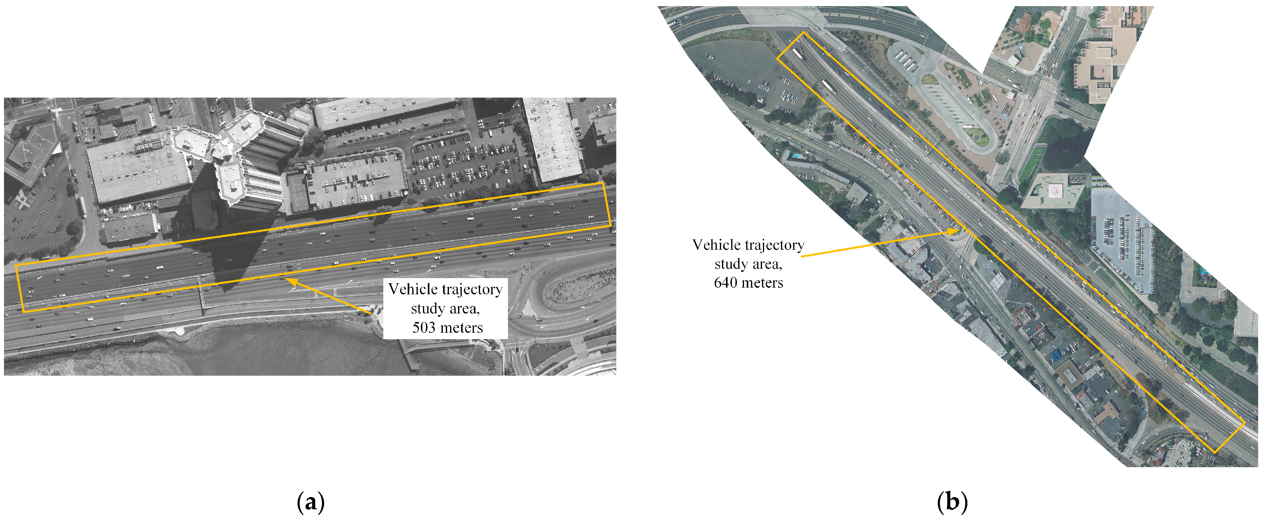
4.1. Evaluation Datasets and Mertics

Our prediction model VTP-GCN was trained and tested on two public vehicle trajectory datasets: I-80 and US-101 in NGSIM [26] which are the most widely used benchmarks for the task of vehicle trajectory prediction. The datasets both contain 45 min vehicle states information (coordinates, velocity, acceleration, etc.) in various traffic scenes with a sampling frequency of 10Hz, and the rich traffic scenes (mild, moderate, and heavy) are suitable for the training and evaluation of the proposed model. The vehicle trajectory study areas of I-80 and US-101 are shown in Figure 5.
For the fairness and effectiveness of the comparison experiments, we followed the data processing method available in the literature [22]: the raw data were downsampled to 5 Hz, and then the trajectories were divided into segments of 8 s each, the first 3 s of which were taken as the historical time horizon to model the interaction among vehicles and the last 5 s were taken as the prediction time horizon to calculate the prediction errors between the predicted trajectories and ground truth data. For the purpose of this paper, the division ratio of training set, verification set, and test set was 6:2:2.
In order to compare the prediction accuracy with the previous excellent vehicle trajectory models, we chose the root mean square error (RMSE) between the prediction trajectory and the ground truth data as evaluation metrics. The smaller the RMSE, the better the prediction accuracy. At the time t h + t , the calculation formula of RMSE is:
R M S E t h + t = 1 N n = i N [ ( x ^ t h + t n x t h + t n ) 2 + ( y ^ t h + t n y t h + t n ) 2 ]
where x t h + t n and y t h + t n are the true position coordinates of a vehicle n at the time t h + t . Since the output of the VTP-GCN is the trajectory distributions, we report the smallest RMSE based on 20 random samplings.

4.2. Implementation Details

Our prediction model was run using Python and Pytorch, and the implementation details are as follows.
(1)
Spatial interaction range: we set the longitudinal spatial interaction range within ±100 m, which is similar to that in Ref [21].
(2)
Input embedding: we used 1 × 1 convolution to increase the number of channels to five, an approach which is beneficial to improve the learning ability of the network.
(3)
Residual connection: the residual connections were introduced in the interaction feature extraction module and the trajectory prediction module to avoid the problems of overfitting and gradient vanishing.
(4)
Training process: the VTP-GCN was trained on the NVIDIA GTX3080 GPU. The batch size and the learning rate were set to 128 and 0.01, respectively. We trained the prediction module for 250 epochs using a stochastic gradient descent (SGD) optimizer.
(5)
Model configuration: to obtain the best prediction accuracy, the number of GCN layers in the interaction feature extraction module and the number of CNN layers in the trajectory prediction module were set to different numbers, so as to select the best model configurations, i.e., two GCN layers and five CNN layers.

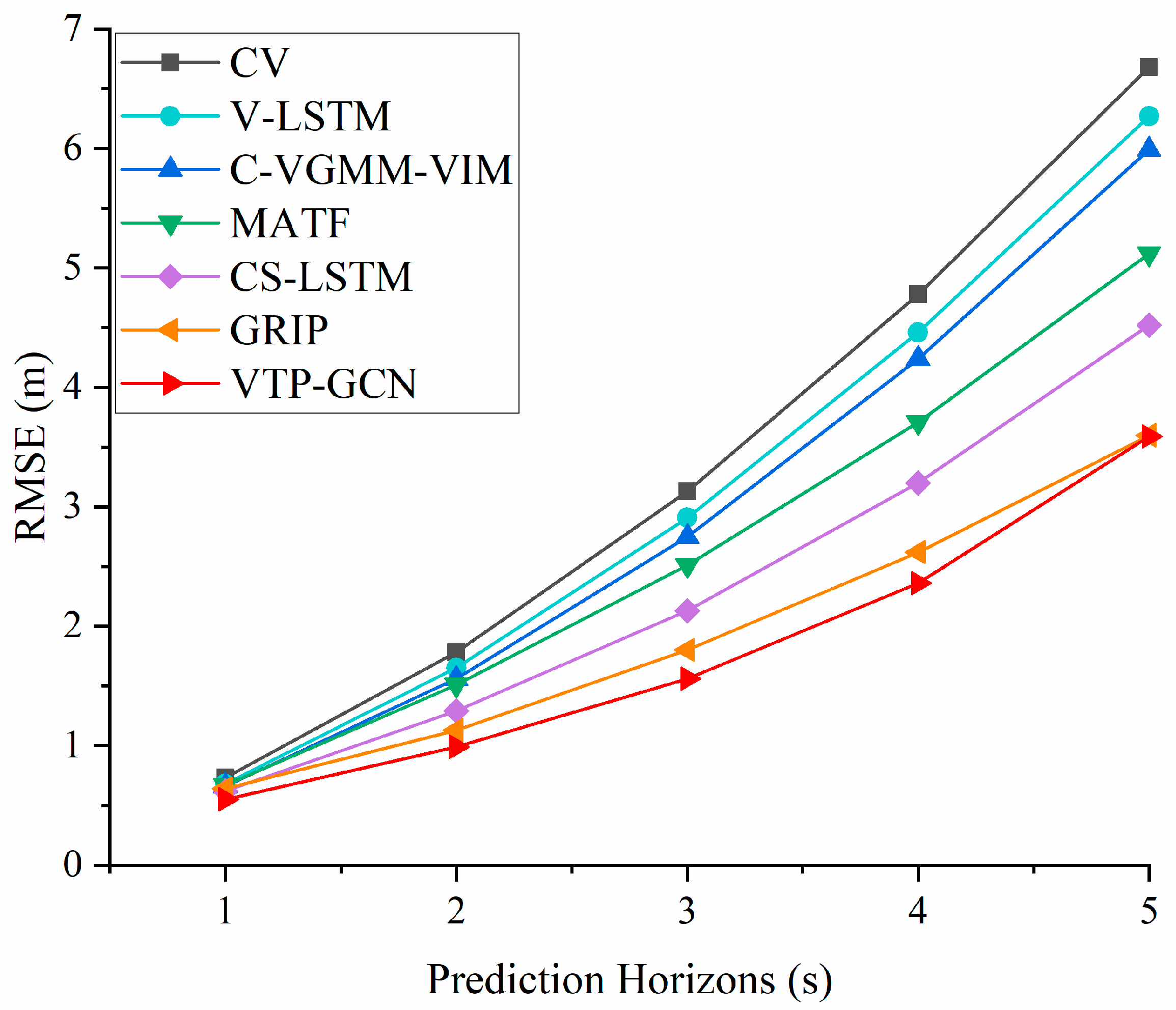
4.3. Quantitative Analysis

In order to evaluate the accuracy of our proposed model, some excellent vehicle trajectory prediction models were selected for quantitative comparison. These were:
(1)
CV: this baseline uses a constant velocity Kalman filter to predict the trajectory of a single vehicle and does not consider the interaction between the predicted vehicle and the surrounding neighbor vehicles.
(2)
V-LSTM: this baseline learns the information hidden in the historical trajectory data based on an LSTM encoder–decoder, and then generates the trajectory distribution of the target vehicle. V-LSTM also does not consider the interdependencies among vehicles.
(3)
C-VGMM+VIM [27]: this baseline first estimates the maneuver intentions based on a hidden markov model (HMM), and then generates the future trajectory based on the variational gaussian mixture models.
(4)
MATF [28]: this baseline encodes the historical trajectory data of vehicles and the information of the driving scene into a multi-agent tensor, and then applies CNNs to extract spatial interactions, decode, and predict the trajectories of all vehicles based on LSTM.
(5)
CS-LSTM: this baseline uses convolutional social pooling as an improvement to social pooling layers to robustly learn spatial interdependencies in vehicle motion.
(6)
GRIP: this baseline uses GCNs to model the spatial–temporal interactions among vehicles and generate the trajectories of all vehicles based on an LSTM encoder–decoder.
We compared the prediction errors of our model with the above baselines on I-80 and US-101 datasets. The RMSE values are shown in Table 1, and the comparison line chart is shown in Figure 6. In Table 1, we can see that the RMSE values of the VTP-GCN model are lower in all prediction horizons, demonstrating the superior spatial–temporal interaction feature modeling ability and future trajectory inference ability of our proposed model. In addition, we found that the baselines (CV, V-LSTM, and C-VGMM-VIM) have larger prediction errors than the models that consider interdependencies, indicating that the interaction information is crucial for the accurate prediction of trajectories. The RMSE values of the models that consider the spatial interactions in the driving scene are reduced, but the trajectory prediction accuracy is still not as good as that of the models considering the spatial–temporal interaction information, showing the necessity of temporal interaction modeling for vehicle trajectory prediction. Although both are vehicle trajectory prediction models based on spatial–temporal interaction modeling, the VTP-GCN model that we proposed attained an 8% average accuracy improvement compared with the GRIP model. That is because we not only improved the modeling of spatial interactions based on the proposed SIC, but also constructed a temporal graph based on raw vehicle data for extracting temporal interactions. The above modifications make the spatial–temporal interaction features obtained by fusion more adequate, while GRIP only extracts interaction features based on the single spatial graph. Therefore, the more effective spatial–temporal interaction feature modeling method helps improve the accuracy of vehicle trajectory prediction.

4.4. Ablation Study

(1)
Spatial Graph with Different Weighted Adjacency Matrices
In this paper, we propose the concept of spatial interaction coefficient and use it as the kernel function to construct a weighted adjacency matrix of the spatial graph to mark the intensity of the spatial interactions between two vehicles within the driving scene. To verify the effectiveness of the above method, the spatial interaction kernel function in the prediction model was modified to the reciprocal of the Euclidean distance. As shown in Table 2, the RMSE values of the SIC-based model are smaller than those of the reciprocal-of-Euclidean-distance-based model at all prediction horizons. Specifically, compared with VTP-GCN, the average RMSE value of the model based on the reciprocal of the Euclidean distance is 5% higher, which proves the effectiveness of the proposed spatial interaction kernel function SIC. The comparison line chart is shown in Figure 7a.
(2)
Temporal Graph with Different Weighted Adjacency Matrices
In order to effectively extract the temporal dependencies of the vehicles, we propose two methods to construct a weighted adjacency matrix of the temporal graph: one based on the reciprocal of the time interval, and one based on the self-attention mechanism. Generally, we think that the influence of the vehicle historical motion state on its current trajectory will weaken as the time interval increases, so we used the reciprocal of the time interval to mark the intensity of temporal interactions. At the same time, the temporal dependency of vehicle is unidirectional, that is, the future trajectory of the vehicle cannot affect the past movement state of the vehicle. Therefore, the weighted adjacency matrix of the temporal graph is defined as:
A t m p _ i = ( 0 1 | Δ T 1 , 2 | 1 | Δ T 1 , 3 | 1 | Δ T 1 , N | 0 0 1 | Δ T 2 , 3 | 1 | Δ T 2 , N | 0 0 0 1 | Δ T 3 , N | 0 0 0 0 )
where Δ T k , q is the difference between the historical time instant k and q . We describe in detail the matrix construction method based on the self-attention mechanism in Section 3.1. (2), and the RMSE values of the prediction models based on the above two methods trained separately are shown in Table 3. The prediction accuracy of the model based on the self-attention mechanism is higher than the other. Specifically, compared with VTP-GCN, the average RMSE value of the model based on the reciprocal of the time interval is 12% higher, meaning that the temporal interaction strength of the vehicle is not linearly related to the time interval, and the method based on self-attention can more fully represent the intensity of temporal interaction. The comparison line chart of the two methods is shown in Figure 7b.
(3)
Effectiveness of Feature Extraction Modules
To validate the effectiveness of the two interaction extraction modules in vehicle trajectory prediction, we trained the two variants of VTP-GCN: VTP-GCN without spatial interaction extraction (variant I: W/O SGCN) and VTP-GCN without temporal interaction extraction (variant II: W/O TGCN). We then compared their prediction results with those from the complete model. The RMSE values of the three models are shown in Table 4. It can be seen from Table 4 that the prediction performance of variant II is superior to that of the complete model at the final prediction horizon. However, VTP-GCN exhibits better prediction accuracy than the two variants at the remaining prediction horizons, exhibiting the smallest RMSE average. It is worth noting that the increase in the average prediction error caused by the absence of the spatial interaction extraction module is larger than that caused by the temporal interaction extraction module, indicating that the spatial interaction behavior of the vehicle within the driving scene has a greater impact on the future motion trajectory of the vehicle compared to the temporal interaction. The comparison line chart of the three methods is shown in Figure 8.

4.5. Qualitative Analysis

The effectiveness of the VTP-GCN proposed in this paper is qualitatively analyzed by visualizing several representative driving scenes using the datasets I-80 and US-101. As shown in Figure 9, the coordinates and velocity data of all vehicles in the scene in the past 3 s are entered into VTP-GCN, and then our model generates the trajectories of the vehicles in the following 5 s.
Figure 9a shows a mild driving scene in which there are no neighboring vehicles that can interact with the predicted vehicle; the predicted vehicle, therefore, chooses to go straight at a high speed. The prediction trajectory of our model fits the solid blue line well, which proves that the proposed model is fully capable of performing vehicle trajectory prediction tasks in simple scenes. In Figure 9b, the traffic density is moderate and there are complex interaction behaviors between vehicles. It is noteworthy that a vehicle in the middle lane will change lanes to the left in search of a better driving experience. Our VTP-GCN accurately predicted the lane change intention, and the error between the predicted trajectory and the ground truth is small. Meanwhile, the predicted trajectories of the rest of the vehicles in this scene are also accurate. In Figure 9c, we show a prediction result in a heavy traffic scene with 13 vehicles. The observation shows that the vehicles in the upper lane move faster, while vehicles in the other lanes drive at relatively slow speeds. Faced with the complex driving scene, our proposed VTP-GCN still predicted the future trajectories of all vehicles accurately. Through the above analysis, we can conclude that the VTP-GCN model that we propose in this paper is applicable to most traffic scenes and that it is able to operate with accuracy and robustness.

5. Conclusions

In this paper, we propose a novel vehicle trajectory prediction scheme, VTP-GCN, in a connected vehicle environment. The model extracts spatial–temporal interaction features in the graph based on GCNs and performs trajectory prediction based on a fully convolutional operation in the temporal dimension. Based on the publicly available datasets I-80 and US-101, the following main conclusions are drawn:
  • The comparative experiment data show that, compared with the baseline models, the vehicle trajectory prediction model VTP-GCN based on graph convolutional neural networks proposed in this manuscript is associated with smaller prediction errors. Specifically, compared with GRIP, the average RMSE value of VTP-GCN is lower by 8%, effectively improving the prediction effectiveness of the future motion trajectories of all vehicles in the driving scene.
  • We model the spatial–temporal interactions among vehicles based on the SIC and the self-attention mechanism. The ablation experiment results of spatial interactions show that the prediction errors of the spatial interaction modeling method based on the traditional reciprocal Euclidean distance are larger, and its average RMSE value increases by 5% compared with the method based on the SIC. The results of the temporal interaction ablation experiment show that the trajectory prediction errors of the temporal interaction modeling method based on the reciprocal of the time interval are larger, and its average RMSE value increases by 12% compared with the method proposed in this study.
  • The ablation experiment data on the effectiveness of the feature extraction module show that the absence of any interaction module will lead to an increase in vehicle trajectory prediction errors. It is worth noting that the absence of SGCN causes the model average prediction error to increase by 6%, while the absence of TGCN causes the model average prediction error to increase by 4%. Therefore, we speculate that spatial interaction modeling is of greater importance than temporal interaction modeling for vehicle trajectory prediction.
In conclusion, the VTP-GCN vehicle trajectory prediction model proposed in this study can model the spatial–temporal interaction behavior among vehicles based on 3 s of historical motion state data, and effectively predict the motion trajectories of all vehicles within the set scene range in the following 5 s. However, the model proposed in this study operates under ideal conditions, that is, we assume that the historical movement data of all vehicles in the scene can be accurately obtained, and does not consider the occlusion, noise, or uncertainty that exist in the networked environment. Therefore, in the subsequent work, we strive to address the issue. At the same time, we will evaluate our prediction model using other datasets, e.g., the HighD dataset or Interaction dataset, in which driving scenes are richer. In addition, we will further enrich the research based on this paper, so that the prediction model can effectively generate the future motion trajectories of all participants in the scenes, including pedestrians and two-wheelers.

Author Contributions

J.S., D.S. and B.G. contributed equally to the formulation of the idea, the design of experiments, the analysis and interpretation of results, and the writing and improvement of the manuscript. All authors have read and agreed to the published version of the manuscript.

Funding

This research was funded by National Natural Science Foundation of China, grant number 52202503. Science and Technology Project of Hebei Education Department, grant number BJK2023026. Hebei Natural Science Foundation, grant number F2022203054.

Institutional Review Board Statement

Not applicable.

Informed Consent Statement

Not applicable.

Data Availability Statement

Conflicts of Interest

The authors declare no conflict of interest.

References

  1. Li, K.; Chang, X.Y.; Li, J.W.; Qing, X.; Bolin, G.; Jian, P. Cloud control system for intelligent and connected vehicles and its application. Automot. Eng. 2020, 42, 1595–1605. [Google Scholar]
  2. Huang, Y.; Du, J.; Yang, Z.; Zhou, Z.; Zhang, L.; Chen, H. A Survey on Trajectory-Prediction Methods for Autonomous Driving. IEEE Trans. Intell. Veh. 2022, 7, 652–674. [Google Scholar] [CrossRef]
  3. Ammoun, S.; Nashashibi, F. Real Time Trajectory Prediction for Collision Risk Estimation between Vehicles. In Proceedings of the IEEE 5th International Conference on Intelligent Computer Communication and Processing (ICCP), Cluj-Napoca, Romania, 27–29 August 2009; pp. 417–422. [Google Scholar]
  4. Jin, B.; Jiu, B.; Su, T.; Liu, H.; Liu, G. Switched Kalman filter-interacting multiple model algorithm based on optimal autoregressive model for manoeuvring target tracking. IET Radar Sonar Navig. 2015, 9, 199–209. [Google Scholar] [CrossRef]
  5. Guo, Y.; Kalidindi, V.V.; Arief, M.; Wang, W.; Zhu, J.; Peng, H.; Zhao, D. Modeling Multi-Vehicle Interaction Scenarios using Gaussian Random Field. In Proceedings of the IEEE Intelligent Transportation Systems Conference (ITSC), Auckland, New Zealand, 27–30 October 2019; pp. 3974–3980. [Google Scholar]
  6. Deng, Q.; Soffker, D. Improved Driving Behaviors Prediction Based on Fuzzy Logic-Hidden Markov Model (FL-HMM). In Proceedings of the IEEE Intelligent Vehicles Symposium (IV), Changshu, China, 26–30 June 2018; pp. 2003–2008. [Google Scholar]
  7. Kiran, B.R.; Sobh, I.; Talpaert, V.; Mannion, P.; Al Sallab, A.A.; Yogamani, S.; Perez, P. Deep Reinforcement Learning for Autonomous Driving: A Survey. IEEE Trans. Intell. Transp. Syst. 2021, 23, 4909–4926. [Google Scholar] [CrossRef]
  8. Fernando, T.; Denman, S.; Sridharan, S.; Fookes, C. Deep Inverse Reinforcement Learning for Behavior Prediction in Autonomous Driving: Accurate Forecasts of Vehicle Motion. IEEE Signal Process. Mag. 2020, 38, 87–96. [Google Scholar] [CrossRef]
  9. Das, K.; Kumar, R.; Krishna, A. Analyzing electric vehicle battery health performance using supervised machine learning. Renew. Sustain. Energy Rev. 2024, 189, 113967. [Google Scholar] [CrossRef]
  10. Das, K.; Kumar, R.; Krishna, A. Supervised learning and data intensive methods for the prediction of capacity fade of lithium-ion batteries under diverse operating and environmental conditions. Water Energy Int. 2023, 66, 53–59. [Google Scholar]
  11. Kumar, R.; Pachauri, R.K.; Badoni, P.; Bharadwaj, D.; Mittal, U.; Bisht, A. Investigation on parallel hybrid electric bicycle along with issuer management system for mountainous region. J. Clean. Prod. 2022, 362, 132430. [Google Scholar] [CrossRef]
  12. Das, K.; Kumar, R. Assessment of Electric Two-Wheeler Ecosystem Using Novel Pareto Optimality and TOPSIS Methods for an Ideal Design Solution. World Electr. Veh. J. 2023, 14, 215. [Google Scholar] [CrossRef]
  13. Zyner, A.; Worrall, S.; Nebot, E. A recurrent neural network solution for predicting driver intention at unsignalized intersections. IEEE Robot. Autom. Lett. 2018, 3, 1759–1764. [Google Scholar] [CrossRef]
  14. Xin, L.; Wang, P.; Chan, C.-Y.; Chen, J.; Li, S.E.; Cheng, B. Intention-Aware Long Horizon Trajectory Prediction of Surrounding Vehicles using Dual LSTM Networks. In Proceedings of the 2018 21st International Conference on Intelligent Transportation Systems (ITSC), Maui, HI, USA, 4–7 November 2018; pp. 1441–1446. [Google Scholar]
  15. Deo, N.; Trivedi, M.M. Convolutional Social Pooling for Vehicle Trajectory Prediction. In Proceedings of the IEEE Conference on Computer Vision and Pattern Recognition (CVPR) Workshops, Salt Lake City, UT, USA, 18–22 June 2018; pp. 1468–1476. [Google Scholar]
  16. Alahi, A.; Goel, K.; Ramanathan, V.; Robicquet, A.; Fei-Fei, L.; Savarese, S. Social LSTM: Human Trajectory Prediction in Crowded Spaces. In Proceedings of the IEEE Conference on Computer Vision and Pattern Recognition (CVPR), Las Vegas, NV, USA, 27–30 June 2016; pp. 961–971. [Google Scholar]
  17. Marchetti, F.; Becattini, F.; Seidenari, L.; Del Bimbo, A. Multiple Trajectory Prediction of Moving Agents with Memory Augmented Networks. IEEE Trans. Pattern Anal. Mach. Intell. 2020, 45, 6688–6702. [Google Scholar] [CrossRef] [PubMed]
  18. Vaswani, A.; Shazeer, N.; Parmar, N.; Uszkoreit, J.; Jones, L.; Gomez, A.N.; Kaiser, Ł.; Polosukhin, I. Attention is All You Need. In Proceedings of the 1st Conference on Neural Information Processing Systems (NIPS 2017), Long Beach, CA, USA, 4–9 December 2017; pp. 5998–6008. [Google Scholar]
  19. Zhao, X.; Chen, Y.; Guo, J.; Zhao, D. A spatial-temporal attention model for human trajectory prediction. IEEE/CAA J. Autom. Sin. 2020, 7, 965–974. [Google Scholar] [CrossRef]
  20. Kim, H.; Kim, D.; Kim, G.; Cho, J.; Huh, K. Multi-Head Attention Based Probabilistic Vehicle Trajectory Prediction. In Proceedings of the IEEE Intelligent Vehicles Symposium (IV), Las Vegas, NV, USA, 19 October–13 November 2020; pp. 1720–1725. [Google Scholar]
  21. Sheng, Z.; Xu, Y.; Xue, S.; Li, D. Graph-based spatial-temporal convolutional network for vehicle trajectory prediction in autonomous driving. IEEE Trans. Intell. Transp. Syst. 2022, 23, 17654–17665. [Google Scholar] [CrossRef]
  22. Li, X.; Ying, X.; Chuah, M.C. GRIP: Graph-Based Interaction-Aware Trajectory Prediction. In Proceedings of the IEEE Intelligent Transportation Systems Conference (ITSC), Auckland, New Zealand, 27–30 October 2019; pp. 3960–3966. [Google Scholar]
  23. Su, Y.; Du, J.; Li, Y.; Li, X.; Liang, R.; Hua, Z.; Zhou, J. Trajectory Forecasting Based on Prior-Aware Directed Graph Convolutional Neural Network. IEEE Trans. Intell. Transp. Syst. 2022, 23, 16773–16785. [Google Scholar] [CrossRef]
  24. Mohamed, A.; Qian, K.; Elhoseiny, M.; Claudel, C. Social-STGCNN: A Social Spatio-Temporal Graph Convolutional Neural Network for Human Trajectory Prediction. In Proceedings of the IEEE/CVF Conference on Computer Vision and Pattern Recognition (CVPR), Seattle, WA, USA, 13–19 June 2020; pp. 14424–14432. [Google Scholar]
  25. Shi, L.; Wang, L.; Long, C.; Zhou, S.; Zhou, M.; Niu, Z.; Hua, G. SGCN: Sparse Graph Convolution Network for Pedestrian Trajectory Prediction. In Proceedings of the IEEE/CVF Conference on Computer Vision and Pattern Recognition (CVPR), Nashville, TN, USA, 20–25 June 2021; pp. 8994–9003. [Google Scholar]
  26. Traffic Analysis Tools: Next Generation Simulation-FHWA Operations. Available online: https://ops.fhwa.dot.gov/trafficanalysistools/ngsim.htm (accessed on 24 November 2020).
  27. Deo, N.; Rangesh, A.; Trivedi, M.M. How Would Surround Vehicles Move? A Unified Framework for Maneuver Classification and Motion Prediction. IEEE Trans. Intell. Veh. 2018, 3, 129–140. [Google Scholar] [CrossRef]
  28. Zhao, T.; Xu, Y.; Monfort, M.; Choi, W.; Baker, C.; Zhao, Y.; Wang, Y.; Wu, Y.N. Multi-Agent Tensor Fusion for Contextual Trajectory Prediction. In Proceedings of the IEEE/CVF Conference on Computer Vision and Pattern Recognition (CVPR), Long Beach, CA, USA, 15–20 June 2019; pp. 12118–12126. [Google Scholar]
Figure 1. The framework of VTP-GCN model.
Applsci 13 13192 g001
Figure 2. An illustration of the spatial interaction range between two vehicles.
Applsci 13 13192 g002
Figure 3. An illustration of the difference between 2D-CNN (a) and GCN (b).
Applsci 13 13192 g003
Figure 4. An illustration of the vehicle trajectory prediction module.
Applsci 13 13192 g004
Figure 5. Bird view of naturalistic traffic recorded within I-80 (a) and US-101 (b) freeway study area.
Applsci 13 13192 g005
Figure 6. Prediction errors of different models.
Applsci 13 13192 g006
Figure 7. Prediction errors of models with different spatial weighted adjacency matrices (a) and different temporal weighted adjacency matrices (b).
Applsci 13 13192 g007
Figure 8. Prediction errors of VTP-GCN and its variants.
Applsci 13 13192 g008
Figure 9. Visualization of predicted trajectories. Green solid lines are the observed history, blue solid lines are the ground truth in the future, red dashed lines are the predicted trajectories (5 s) generated by our VTP-GCN. (a) Only one vehicle with temporal dependencies, (b) seven vehicles in a moderate traffic scene in which a vehicle will engage in lane changing, (c) thirteen vehicles in a heavy traffic scene with complex spatial–temporal dependencies.
Applsci 13 13192 g009aApplsci 13 13192 g009b
Table 1. RMSE values for vehicle trajectory prediction using I-80 and US-101 datasets. Data are converted into meters. The performance of models denoted by * is published in [21,22]. All results except ours are extracted from previous studies. The smaller the RMSE value, the better the prediction accuracy.
Prediction Horizon (s)CV *V-LSTM *C-VGMM-VIM *MATF *CS-LSTM *GRIP *VTP-GCN
(∆GRIP)
10.730.680.660.670.620.640.55 (↓14%)
21.781.651.561.511.291.130.99 (↓12%)
33.132.912.752.512.131.801.56 (↓13%)
44.784.464.243.713.202.622.36 (↓9%)
56.686.275.995.124.523.603.59 (↓0%)
Average3.423.303.042.702.351.961.81 (↓8%)
Table 2. Comparison of RMSE values for models with different spatial weighted adjacency matrices. Data are converted into meters.
Prediction Horizon (s)12345
1 D 0.63(+0.08)1.08(+0.09)1.65(+0.09)2.43(+0.07)3.73(+0.04)
S I C 0.550.991.562.363.59
Table 3. Comparison of RMSE values for models with different temporal weighted adjacency matrices. Data are converted into meters.
Prediction Horizon (s)12345
Reciprocal of time interval0.72(+0.17)1.23(+0.24)1.79(+0.23)2.57(+0.21)3.80(+0.21)
Self-attention0.550.991.562.363.59
Table 4. Comparison of RMSE values for the variants of VTP-GCN. Data are converted into meters.
Prediction Horizon (s)W/O SGCNW/O TGCNVTP-GCN
10.62(+0.07)0.67(+0.12)0.55
21.05(+0.06)1.16(+0.17)0.99
31.63(+0.07)1.69(+0.13)1.56
42.48(+0.12)2.40(+0.04)2.36
53.82(+0.23)3.49(−0.10)3.59
Average1.92(↑6%)1.88(↑4%)1.81
Disclaimer/Publisher’s Note: The statements, opinions and data contained in all publications are solely those of the individual author(s) and contributor(s) and not of MDPI and/or the editor(s). MDPI and/or the editor(s) disclaim responsibility for any injury to people or property resulting from any ideas, methods, instructions or products referred to in the content.

