Optimal Control for a Three-Rotor Unmanned Aerial Vehicle in Programmed Flights

Abstract

In this study, we propose a new approach to selecting PID controller parameters for a UAV tricopter during programmed flights. The approach uses optimization techniques to determine the optimal values of the PID controller parameters based on the desired performance of the UAV. The proposed method is particularly effective for repeated programmed flights in which the UAV follows a defined flight path. The use of a PID control provides a reliable and robust control system that can cope with various disturbances and uncertainties in UAV dynamics. The proposed method provides an alternative to adaptive control, which requires a significant amount of system identification and parameter tuning. The effectiveness of the proposed method has been verified in simulation studies, and the results show its ability to achieve satisfactory performance with low tracking error and fast response time. The result of the work is an improvement in control for a specific object at a specific mission. We present how the recipients can perform this procedure for their object and their mission to be able to improve the control gain in the physical controller.

1. Introduction

Unmanned aerial vehicles are the subject of many publications, and their applications are growing every year. New possibilities for implementing this technology to improve various areas of life, such as medical rescue [1], management of large buildings [2] and their inspection [3], creating models of existing buildings [4] and their assessment [5], as well as for public safety by state authorities [6], are being discovered. Due to the responsibility and complexity of the tasks performed, reliable and mission-adapted flying objects are necessary.

The quadcopter is the most popular type of multi-rotor unmanned aerial vehicle (UAV). There are many scientific articles available on its control [7] and dynamics [8]. The tricopter, which uses three motors to generate thrust, is a much less common type of UAV in the literature. It requires a suitable design due to the odd number of motors. Examples of using a tricopter with a tail servo [9] or without [10] can be found in the literature. Scientists have mainly focused on design projects [11] and construction [12] of tricopters, with less attention given to simulation studies of their flight dynamics. The literature on modeling this type of object does not provide sufficient attention to control and quality regulation. Sababha Belal et al. [13] presented simulations of the motion of a tricopter in their work but did not indicate how to choose the coefficients of regulators for this type of object. Daniel Abara has focused his dissertation [14] on considering what type of controller is best for a tricopter-type object. However, he did not consider the universality of the implementation of the controller types in question and the possibility of tuning their parameters to the needs of users. On the other hand, the authors of the paper [15], subjecting to their considerations an object of the tricopter type, considered a design that is not commonly used due to the lack of a tail servo. The tail servo not only makes it difficult to consider the control of this object but also provides opportunities for better control during dynamic movements. In a number of papers, including [16], the authors have considered the control of the chosen design but have not considered the choice of controller settings depending on the mission to be performed by the UAV. Most of the research conducted does not focus on using the tricopter to perform a specific task but only on experiments testing the correctness of derived models [10]. The authors believe that there is a gap in the optimization of program flights and the methodology for selecting tricopter regulator gains for program flights presented in this paper.

The authors of this paper addressed the issue of selecting proportional–integral–derivative (PID) regulator parameters for tricopters for altitude, rotational, and linear motion, which, according to the authors’ current knowledge, has not yet been accomplished using the proposed method. The choice of the type of regulators was conditioned by its common implementation in flight control software such as PX4, ArduPilot, and BetaFlight. Common optimization methods were used to achieve the intended goal of selecting parameters. The use of optimization methods for all gains of specific trajectories is innovative. The authors first considered which optimization method is best, for example, a hovering task. They then proceeded to use the best optimization method to realize specific trajectories that may be useful for, for example, monitoring buildings. The author’s contribution to the paper was to optimize controller coefficients not for general tasks but to consider individual tasks and present a procedure for how the recipients of this paper can perform optimizations not only for their object but for a specific object and a specific trajectory, which has not been the subject of research work before.

A computer-aided design (CAD) modeled object that can be printed in 3D was used in this paper. We hypothesized that in order to select optimal gains for a tricopter, it is necessary to do this separately for each program task. This is a method similar to adaptive control, but it requires much greater computational complexity, so an optimizing simulation must be performed first, and the received gains should be loaded into the tricopter controller. Attention was focused on the quality of the control system, for which the criterion of the integral of the absolute error value was used for evaluation. The PID controller tuning was performed using the “control systems” toolbox in Matlab R2023a to determine the initial values, and optimization functions were also used to improve the quality of regulation. Simpler types of control algorithms, which can be obtained by zeroing individual PID controller settings, such as PD and PI, are also taken into account during the optimization process. Controllers of this type are considered in the paper due to their ubiquity in implementation in commercially available flight controllers. Adjustment values can be corrected in them, but the control structure cannot be changed to another type of controller. The aim of the paper is to provide a scheme of operation that the reader can use to improve regulation on their own object.

The structure of the paper is as follows: Section 2 is devoted to the topic of the tricopter objects and their advantages and disadvantages as an unmanned object are discussed. The physical model is presented, followed by the mathematical model of the specific object. Section 3 presents the issue of control and a possible way of implementation. The methods used for tuning the PID controller coefficients are explained, and the evaluation indicator for the regulation quality used in the research is presented. Section 4 contains simulation results in graphical form. They show the object’s response to the specified angular and linear position values. This chapter is organized into subsections in which the different scenarios are analyzed together with their qualitative assessment. Section 5 is a discussion of the results, including a summary of the paper and an assessment of the usefulness of the presented results.

2. Control Object

2.1. Tricopter Characteristics

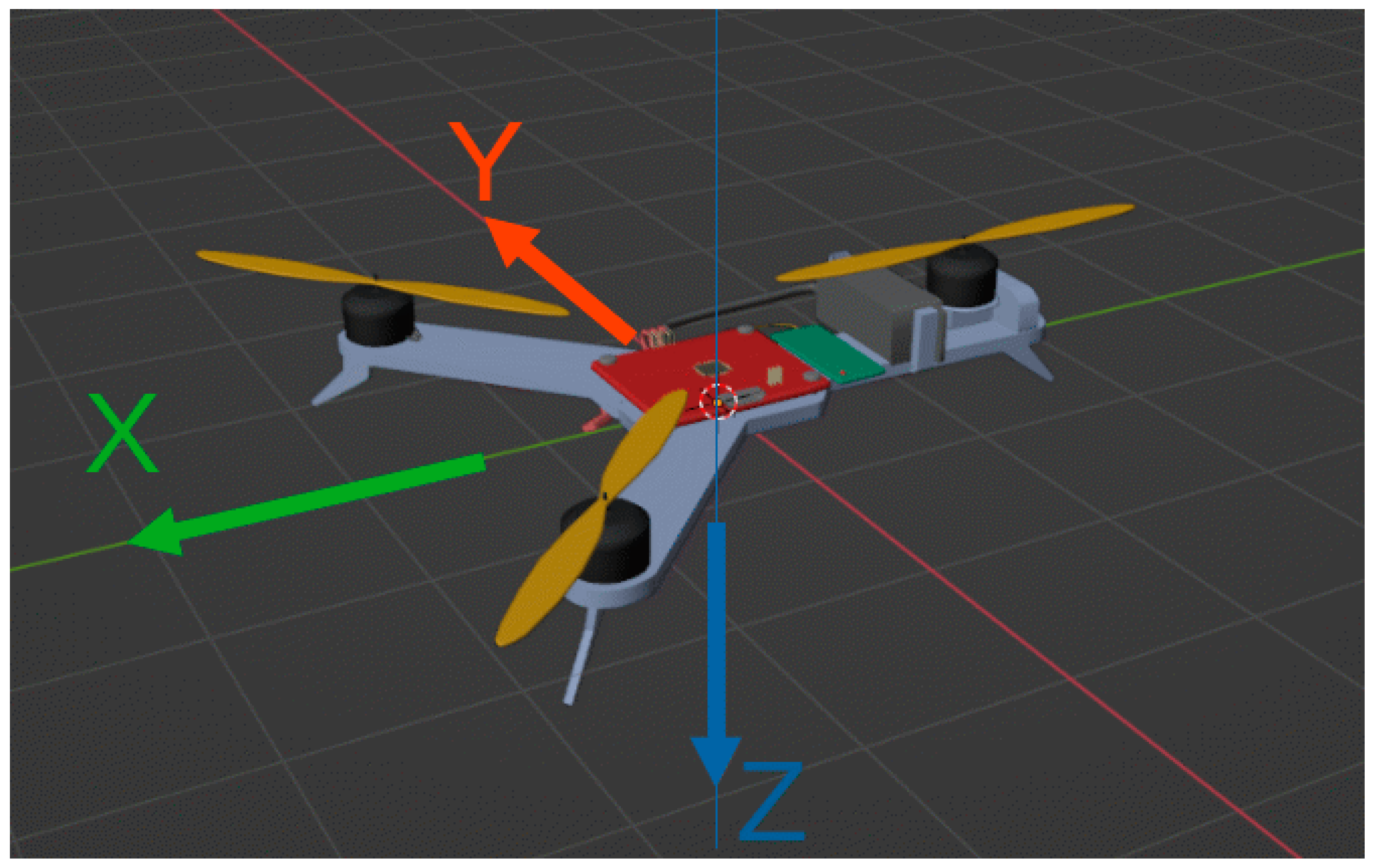
The tricopter is a highly complex object in terms of its construction [12] and, consequently, also in terms of control. With the increasing interest in this type of unmanned flying object, it has received support in the flight controller software of the most popular open-source distributions (Figure 1).

Depending on the concept adopted, the motors may rotate in the same direction or in a configuration where two rotate in one direction and the third in the opposite direction. As mentioned in the introduction, a servo is used on the tail, whose task is to rotate the motor around the tricopter’s tail axis. This is necessary to balance the gyroscopic moments generated by the motor movements during operation. In objects without a servo [10], the object will rotate minimally around its axis while hovering. However, in the presence of a servo and motor rotation on the tail, an additional force is present, which is further discussed in Section 4.2.

Comparing tricopters with other multirotor UAVs, such as quadcopters, we can say that their complexity is one of their drawbacks. Also, in terms of landing maneuver, the tricopter’s structure is less stable and, as a result, less durable. Due to the smaller number of motors, its payload capacity is also reduced, but the lower number of motors translates into a lower cost for the entire object, which is usually lower in the case of tricopters. Additionally, the weight of the object is lower than that of a quadrotor, which translates into longer battery life during flight. With the additional servo, the maneuverability in the z-axis (yaw angle) is increased. The analyzed tricopter is presented in the figure below (Figure 2).

The concept was adopted in which the angle of the tail motor can be changed by a servo mechanism. The two remaining motors rotate in opposite directions. By shifting the center of mass closer to the front of the tricopter, the need to apply a large angle of deflection to the tail motor has been reduced.

2.2. Physical Model

The adopted reference frame is the one related to the object. The Z-axis is directed towards the Earth (Figure 3).

It has been assumed that the thrust forces and rotational moments generated by individual motors are proportional to the square of the motor speed value [19]. The coefficients determining the thrust force and rotational moment values can be expressed by the following equation:

$$f_i=k_t·{\omega }_i^2,$$

(1)

$${\tau }_i=k_d·{\omega }_i^2,$$

(2)

where:

• τ_i—torque,
• f_i—thrust force,
• k_t—thrust coefficient,
• k_d—torque coefficient,
• ω_i—motor speed,
• i—motor numer {1, 2, 3}.

Similarly to the commonly used equations for a quadcopter [20], the control forces for a tricopter are expressed as:

$$U_z=-k_t{\omega }_1^2-k_t{\omega }_2^2-k_t{\omega }_3^{2}cos\left(\alpha \right),$$

(3)

$$U_{\varphi }=-d_1{k}_t{\omega }_1^2+d_1{k}_t{\omega }_2^2,$$

(4)

$$U_{\theta }=d_2{k}_t{\omega }_1^2+d_2{k}_t{\omega }_2^2-d·k_t{\omega }_3^{2}cos\left(\alpha \right),$$

(5)

$$U_{\psi }=-k_d{\omega }_1^2-k_d{\omega }_2^2-k_d{\omega }_3^{2}cos\left(\alpha \right)+d{·k}_t{\omega }_3^{2}sin\left(\alpha \right),$$

(6)

where:

• U_z—thrust force,
• U_Φ—rotation force around the X-axis,
• U_θ—rotation force around the Y-axis,
• U_ψ—rotation force around the Z-axis,
• d₁—distance between the center of the tricopter and the right or left motor, measured in the Y-axis,
• d₂—distance between the center of the tricopter and the right or left motor, measured in the X-axis,
• d—distance between the center of the tricopter and the tail motor,
• α—angle of inclination of the tail motor.

In addition, there is a fifth force resulting from the inclination of the tail motor, called $U_Y$. It is equal to:

$$U_Y={k_t\omega }_3^{2}sin\left(\alpha \right).$$

(7)

To minimize this force, it is important for the right and left motors to rotate in opposite directions and for the center of mass to be shifted forward.

The flight controller on board the tricopter is responsible for generating the desired engine speeds and tail motor angles. The equations derived by the authors from Equations (3)–(7) are as follows:

$${\omega }_1=\sqrt{\frac{-d}{2k_t\left(d+d_2\right)}{U}_z-\frac{1}{2d_1{k}_t}{U}_{\varphi }+\frac{1}{2k_t\left(d+d_2\right)}{U}_{\theta }},$$

(8)

$${\omega }_2=\sqrt{\frac{-d}{2k_t\left(d+d_2\right)}{U}_z+\frac{1}{2d_1{k}_t}{U}_{\varphi }+\frac{1}{2k_t\left(d+d_2\right)}{U}_{\theta }},$$

(9)

$${\omega }_3=\sqrt[4]{\frac{\left[k_t^2{U}_{\psi }^2{\left(d+d_2\right)}^2+k_d^2{U}_z^2{\left(d+d_2\right)}^2-2k_t{k}_d{U}_{\psi }{U}_z{\left(d+d_2\right)}^2+d_2^2{U}_z^2{k}_t^2{d}^2+U_{\theta }^2{k}_t^2{d}^2+2d_2{U}_z{U}_{\theta }{k}_t^2{d}^2\right]}{\left(d^2{k}_t^4{\left(d+d_2\right)}^2\right)}},$$

(10)

$${cos}^2\alpha =\frac{\left(d_2^2{U}_z^2+U_{\theta }^2+2d_2{U}_z{U}_{\theta }\right)}{k_t^2{\left(d+d_2\right)}^2{·\omega }_3^4}.$$

(11)

2.3. Mathematical Model

The tricopter is treated as a rigid body with a mass m, and the total force acting on it is the sum of the force generated by the rotors and the force due to gravity. The equations of motion derived using the Newton–Euler method derived by reference [20], only for a tricopter-type object are:

$$\begin{array}{c}\ddot{x}=\frac{1}{m}\left[U_y\right(sin\left(\varphi \right)\mathrm{s}\mathrm{i}\mathrm{n}\left(\theta \right)\cos \left(\psi \right)-cos\left(\varphi \right)\sin \left(\psi \right))+U_z(\mathrm{s}\mathrm{i}\mathrm{n}\left(\theta \right)cos\left(\varphi \right)\cos \left(\psi \right)+\\ sin\left(\varphi \right)\sin \left(\psi \right)\left)\right],\end{array}$$

(12)

$$\begin{array}{c}\ddot{y}=\frac{1}{m}\left[U_y\right(sin\left(\varphi \right)\mathrm{s}\mathrm{i}\mathrm{n}\left(\theta \right)\sin \left(\psi \right)+cos\left(\varphi \right)\cos \left(\psi \right))+U_z(\mathrm{s}\mathrm{i}\mathrm{n}\left(\theta \right)cos\left(\varphi \right)\sin \left(\psi \right)-\\ sin\left(\varphi \right)\cos \left(\psi \right)\left)\right],\end{array}$$

(13)

$$\ddot{z}=\frac{1}{m}[U_{y}sin\left(\varphi \right)cos\left(\theta \right)+U_{z}cos\left(\varphi \right)\cos \left(\theta \right)+mg],$$

(14)

$$\ddot{\varphi }=\frac{1}{J_{xx}}\left[\right(J_{yy}-J_{zz})\dot{\theta }\dot{\psi }+U_{\varphi }],$$

(15)

$$\ddot{\theta }=\frac{1}{J_{yy}}\left[\right(J_{zz}-J_{xx})\dot{\varphi }\dot{\psi }+U_{\theta }],$$

(16)

$$\ddot{\psi }=\frac{1}{J_{zz}}\left[\right(J_{xx}-J_{yy})\dot{\varphi }\dot{\theta }+U_{\psi }],$$

(17)

where:

• J_xx—moment of inertia about the X-axis,
• J_yy—moment of inertia about the Y-axis,
• J_zz—moment of inertia about the Z-axis.

Since the experiments generally involve the tricopter operating close to the hover point, the linear equations of motion (12)–(17) can be linearized. It is assumed that $\varphi \approx 0$, $\theta \approx 0$, so $\sin \left(\varphi \right)\approx 0,\sin \left(\theta \right)\approx 0$, $\cos \left(\varphi \right)\approx 0,\cos \left(\theta \right)\approx 1$. In addition, based on [20], it can be assumed that the initial speed of the motors is the speed at which the object is maintained at the desired altitude:

$$U_z=-mg+\mathsf{\Delta }{U}_z,$$

(18)

where:

• ΔU_z—required control to keep the UAV hovering.

Using Equation (18), we can derive the following equations of linear and spherical motion:

$$\ddot{x}=-g·\theta ,$$

(19)

$$\ddot{y}=g·\varphi +\frac{U_Y}{m},$$

(20)

$$\ddot{z}=\frac{U_z}{m}+g,$$

(21)

$$\ddot{\varphi }=\frac{U_{\varphi }}{J_{xx}},$$

(22)

$$\ddot{\theta }=\frac{U_{\theta }}{J_{yy}},$$

(23)

$$\ddot{\psi }=\frac{U_{\psi }}{J_{zz}}.$$

(24)

3. Control and Optimization

The experimental parameter is the ascent of the tricopter to a height of 0.5 m. The control system diagram created in Simulink program is presented in Figure 4.

The individual blocks correspond to the tricopter control elements and model its dynamics. The “reference velocities” block, together with the PID controller, performs the flight controller’s tasks by generating rotational speeds for all motors. The next block generates control signals. These signals are processed by “linear motion” and “rotational motion” blocks, which include modeled tricopter dynamics.

Using a dedicated toolbox and the PID tuner function [21], the initial gains for the PID controller controlling the height of the tricopter were selected. The PID tuner block (Figure 5) allows for optimizing the gains for a given controller during simulation.

The authors then proceeded to select gains using optimization methods. The following methods were used: fmincon, fminimax, lsqnonlin, and fminsearch [22]. Fmincon is a function that finds the minimum of a constrained function using a quasi-Newton algorithm that makes quadratic approximations at each iteration. Fminimax uses the sequential quadratic programming (SQP) method, which solves a sequence of quadratic programming subproblems. Lsqnonlin is a function that finds the minimum using the Levenberg–Marquardt algorithm, which makes a linear approximation at a large distance from the minimum and a quadratic approximation in the vicinity of the minimum. Fminsearch finds the minimum of an unconstrained function using the Nelder–Mead simplex method, which does not use function derivatives. In this method, constraints were imposed programmatically.

The integral of the absolute error criterion (IAE) was used to evaluate the control quality:

$$J=\underset{-\mathrm{\infty }}{\overset{\mathrm{\infty }}{\int }}f\left(\right|e\left(t\right)|,t)dt,$$

(25)

where:

• J—calculated error,
• e(t)—error,
• t—time.

This criterion was chosen based on available literature [23] as the most suitable for a measurable assessment of control quality.

To achieve the goal of selecting PID controller parameters, an optimization function was called to search for three gains for the altitude controller.

$$\begin{array}{c}\left[{Kp}_z,{Ki}_{z },{Kd}_z\right]=\\ fmin\left(tricopter dynamic function,PID starting parameters,options\right),\end{array}$$

(26)

where:

• Kp_z, Ki_z, Kd_z—sought altitude PID controller gains,
• fmin—optimization function called as minimizing the IAE error,
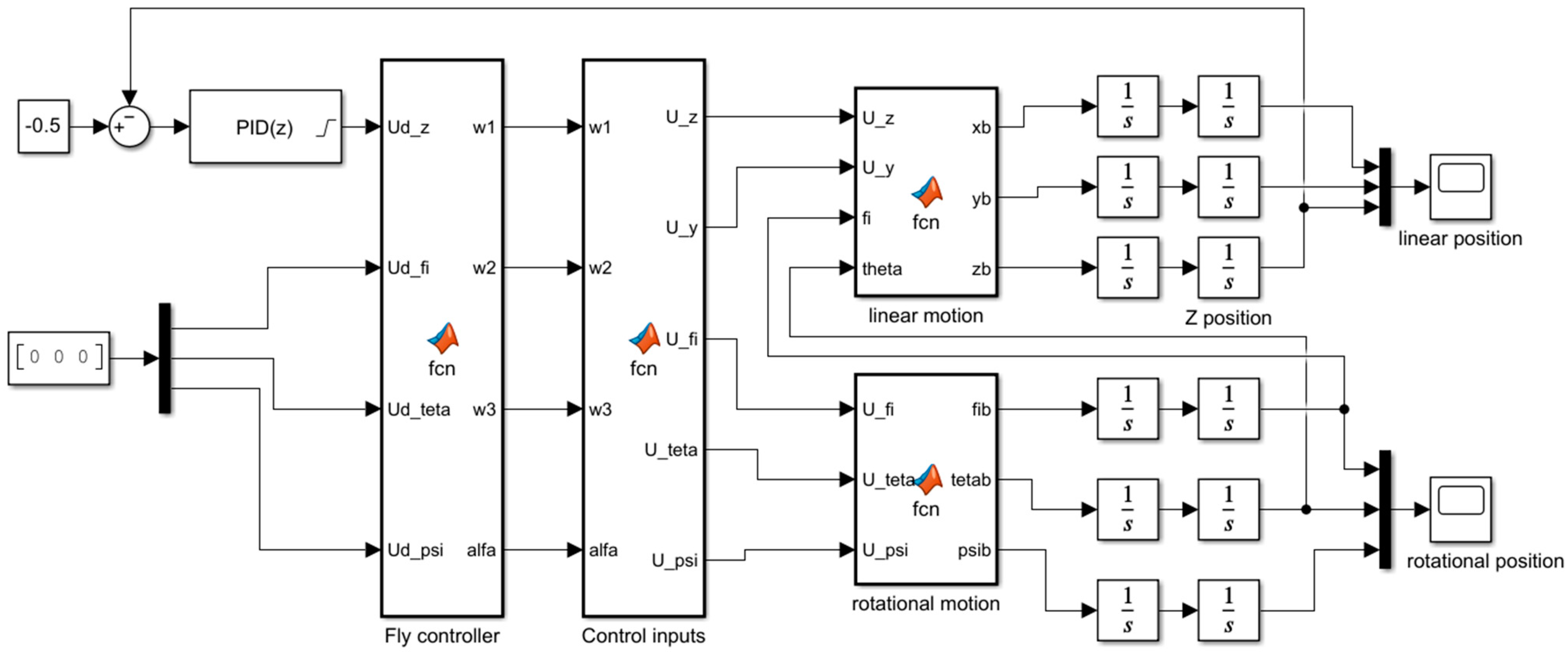
• tricopter dynamic function—modeled dynamics, graphically presented in Figure 4,
• starting parameters—initial gains selected using PID Tuner,
• options—simulation parameters, responsible for, among other things, the number of iterations.

Each of the optimization functions described above—fmincon, fminimax, lsqnonlin, and fminsearch—was called in sequence using fmin. The comparison of the obtained results is presented in tabular form in Section 4.2. Subsequent experiments, in which values for the remaining controllers were selected, were performed analogously to Equation (26), with the difference that gains for all controllers were searched for. In this case, the optimization function takes the form:

$$\begin{array}{r}\left[{Kp}_x,{Ki}_{x },{Kd}_{x },{Kp}_y,{Ki}_{y },{Kd}_y,{Kp}_z,{Ki}_{z },{Kd}_{z },{Kp}_{\varphi },{Ki}_{\varphi },{Kd}_{\varphi },{Kp}_{\theta },{Ki}_{\theta },{Kd}_{\theta },{Kp}_{\psi },{Ki}_{\psi },{Kd}_{\psi }\right]\\ \hspace{1em}\hspace{1em}=fmin\left(tricopter dynamic function,PID starting parameters,options\right).\end{array}$$

(27)

The structure of the optimization methods allows for searching for the minimum based on a single error criterion. To use the optimization methods, weights were assigned to each value controlled by PID.

$$w_x+w_y+w_z+w_{\varphi }+w_{\theta }+w_{\psi }=1$$

(28)

By using weights, it is possible to obtain a single output for the minimization function. The values of individual weights were selected for each experiment by searching the space, taking into account the authors’ experience in flight.

4. Results

4.1. Simulation Parameters

The simulation studies were carried out in Matlab with a constant integration step of 0.001, using the ode3 method. Moments of inertia, together with tricopter parameters, were obtained from the CAD model using SolidWorks 2022 software. The maximum motor speed, ${\omega }_{max}$, was limited.

Table 1. Tricopter parameters.

Parameters	Value
d	0.1625 m
d1	$\sqrt[]{2d}$
d2	0.5d
m	0.703 kg
kt	1.591 × 10−6 kg·m
kd	2.354 × 10−8 kg·m2
Jxx	2.33 × 10−3 kg·m2
Jyy	2.71 × 10−3 kg·m2
Jzz	4.36 × 10−3 kg·m2
ωmax	1440 rad/s

presents a summary of the adopted tricopter parameters. All the methods of selecting regulator gains and the obtained control effects were compared with the settings of the ArduPilot 4.4.2 software and the results obtained for them.

The speed was limited to 90% of the speed of 1600 rad/s, which is the maximum for the used motors powered by a three-cell battery.

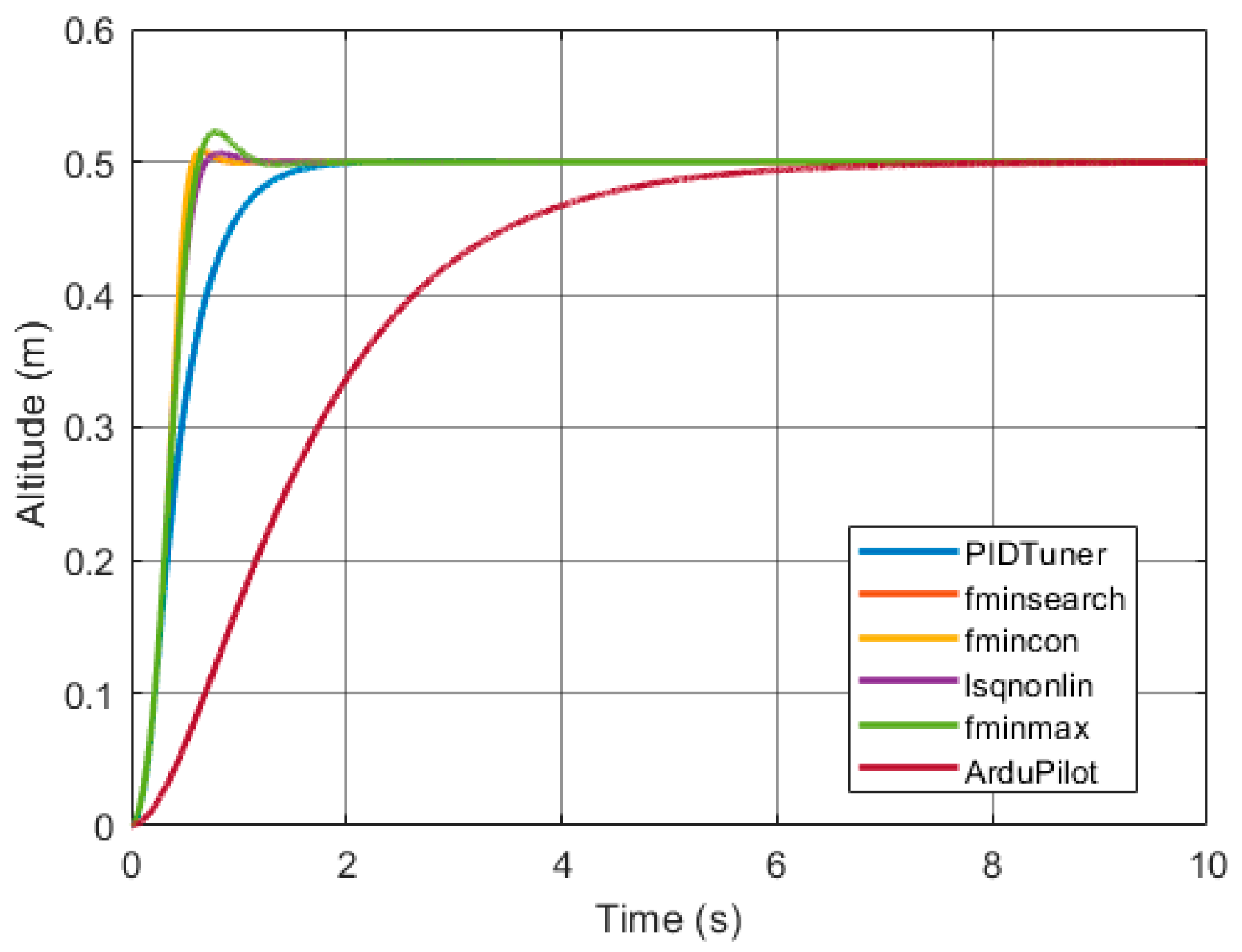
4.2. Tricopter Hovering at Desired Height

4.2.1. Conditions of the Experiment

The first task was to perform a tricopter flight at a height of 0.5 m and to select optimal PID controller coefficients only for controlling the altitude of the object. In this case, the weights for optimization methods can be presented as follows:${ w}_z=1$, $w_x,w_y,w_{\varphi },w_{\theta },w_{\psi }=0.$

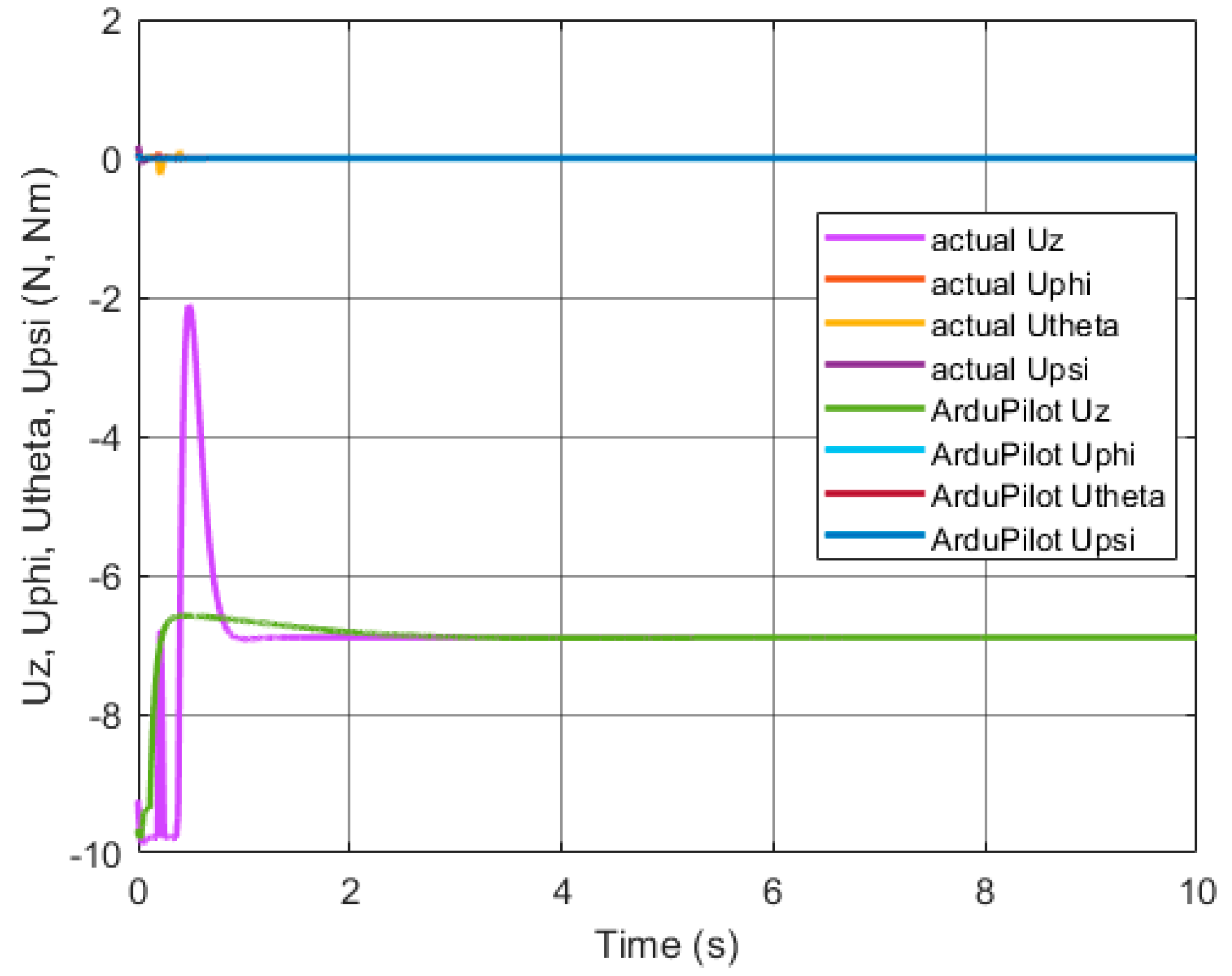
4.2.2. Simulation Studies and Summary of the Experiment

The results presented in Figure 6 are similar to each other. To better compare the effect of selecting gains on the quality of regulation, the data was collected in tabular form.

Table 2. Selected PID regulator gains and comparison of regulation quality according to the specified criterion.

Method of Selection	ArduPilot	Fminsearch	Fmincon	Lsqnonlin	Fminimax	PID Tuner
The selected coefficient Kp	42	138.32	42.99	55.76	42.98	54.95
The selected coefficient Ki	3.5	41.58	41.31	41.61	41.29	48.22
The selected coefficient Kd	7	14.79	7.44	8.67	7.44	15.25
IAE	3.934	0.168	0.181	0.176	0.181	0.241

presents a summary of all the methods for selecting the PID height regulator parameters for the tricopter, together with the obtained gains. The last row contains a comparison according to the previously mentioned IAE criterion. The result obtained by the fminsearch was the best. The results of fmincon, lsqnonlin, and fminimax methods were almost identical. Despite the worst results according to the specified criterion, the PID tuner allowed for object control without overshooting, although it should be noted that in the case of other methods, this overshooting is slight and was particularly small when using the fminsearch method.

Taking the above into account, in the following simulation studies presented in the next sections, the fminsearch method was used to select the parameters of the PID gains because of its quality.

4.3. Height and Rotational Movement Regulator

4.3.1. Conditions of the Experiment

The tricopter’s task was to fly at a constant height while maintaining constant rotation angles. The set values assumed were: height 0.5, pitch angle 1 degree, roll angle 1 degree, and yaw angle 1 degree. The weights for optimization methods were as follows: $w_z=0.6$, $w_x,w_y=0$, $w_{\varphi },w_{\theta }=0.$1, and $w_{\psi }=0.2$. They were selected based on the authors’ flight experiences. The gains of ArduPilot, as in the previous example, were downloaded from the controller after appropriate configuration.

4.3.2. Simulation Studies and Summary of the Experiment

Figure 7, Figure 8, Figure 9, Figure 10, Figure 11 and Figure 12 show the responses of the modeled drone system. As can be seen, it reaches the set values in less than one second. The PID controller coefficients selected by optimization are presented in

Table 3. Controller gains for height and rotational position control.

Variable	Kp	Ki	Kd
Altitude	102.16	38.61	14.38
Roll	7.75	0.03	0.33
Pitch	28.11	0.00	0.19
Yaw	61.73	0.00	1.31

.

The tricopter with optimized gains completed the task in approximately 0.5 s. From this point in time, the value of the control signals stabilizes at a constant level. Looking at Table 3, it can be concluded that PD controllers are optimal for pitch and yaw angles for the considered task. Comparatively, the ArduPilot only reached the set altitude after 4.5 s. Its dynamics are slightly less responsive, which translates into time to complete the set mission. The integral of the absolute value of the error for the settings selected during optimization was 0.434, while for the simulation with the ArduPilot settings, it was 4.245.

4.4. Spiral Flight

4.4.1. Desired Trajectory and Conditions of the Experiment

The next task is a simulation of a real task that UAVs often have to cope with. The tricopter is to perform an ascending flight along a spiral with a constant radius. The trajectory is planned in advance. To place the task in real conditions, the tricopter starts at a random point, which does not have to coincide with the beginning of the trajectory. This is to simulate a situation where we plan for the UAV to patrol a skyscraper by taking off, circling it several times, and creating a spiral. The starting point of the desired trajectory is constant, while the launch point of the tricopter may differ in each repetition.

The equations determining the form of the desired trajectory were as follows [24]:

$$z_d\left(t\right)=t,$$

(29)

$$x_d\left(t\right)=2\sin \left(\frac{2\mathsf{\pi }}{30}t\right),$$

(30)

$$y_d\left(t\right)=2\sin \left(\frac{2\mathsf{\pi }}{30}t-\frac{\mathsf{\pi }}{2}\right),$$

(31)

$${\psi }_d\left(t\right)=\mathsf{\pi }\sin \left(\frac{2\mathsf{\pi }}{30}t\right).$$

(32)

Based on the previously described procedure for selecting PID controller parameters, parameters for position controllers were selected. These are gains selected for a specific task described above. The weights for optimization methods were as follows: $w_z=0.4$, $w_x,w_y=0.1$, $w_{\varphi },w_{\theta }=0.$1, and $w_{\psi }=0.2$ (see Equation (28)).

The selected gains are shown in

Table 4. Controller gains for spiral flight.

Variable	Kp	Ki	Kd
X	6.98	4.73	3.45
Y	6.78	4.23	4.26
Altitude	80.47	59.28	10.76
Roll	7.41	0.00	0.26
Pitch	13.08	12.10	1.47
Yaw	3.07	0.00	0.66

.

The gains for the ArduPilot were the same as in the previous experiment—downloaded from the controller. The gains for the X and Y controllers were taken from the Table above.

4.4.2. Simulation Studies and Summary of the Experiment

The simulation results are presented in Figure 13, Figure 14, Figure 15, Figure 16, Figure 17, Figure 18, Figure 19, Figure 20 and Figure 21.

Additional constraints adopted for this experiment are the tilt and tilt angles, which, due to the tricopter’s design, were assumed not to exceed the range of −20 degrees to 20 degrees. During the simulation, the UAV followed the planned trajectory after 5 s and continued to follow it. The trajectory was planned so that the UAV could use 2/3 of its power while following it. This allowed the UAV to initially catch up to the planned trajectory by using the power reserve. The control signals $U_{\varphi },U_{\theta },U_{\psi }$ were small. The object has flown stably since the beginning of the experiment. Compared with the experiment obtained from the ArduPilot gains, it can be concluded that the settings selected by the optimizers for the specific task were better. When comparing using the IAE criterion, an improvement from 8.546 to 0.589 was obtained. This is mainly due to the start of the maneuver, which was executed much more efficiently using the specially selected gains.

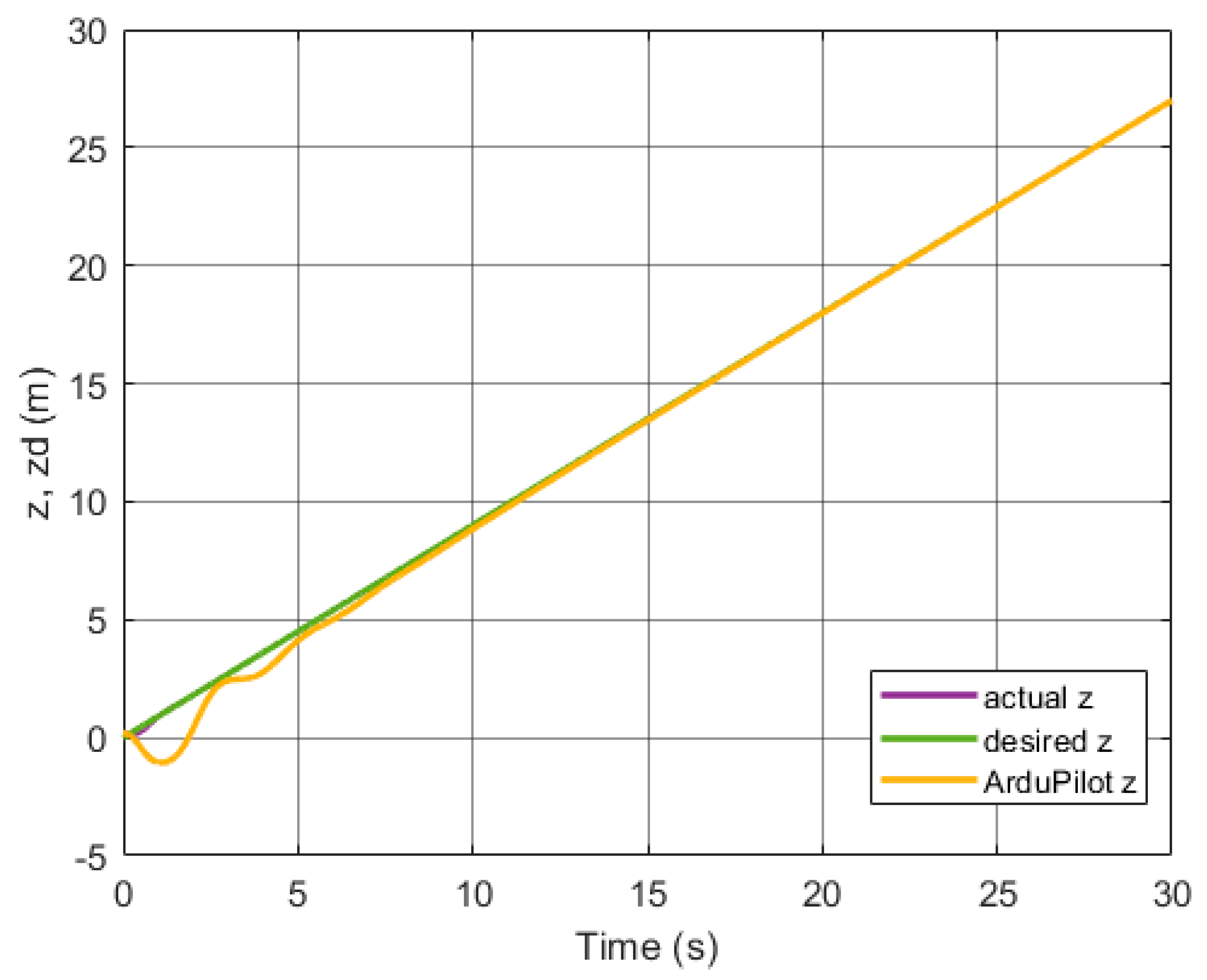
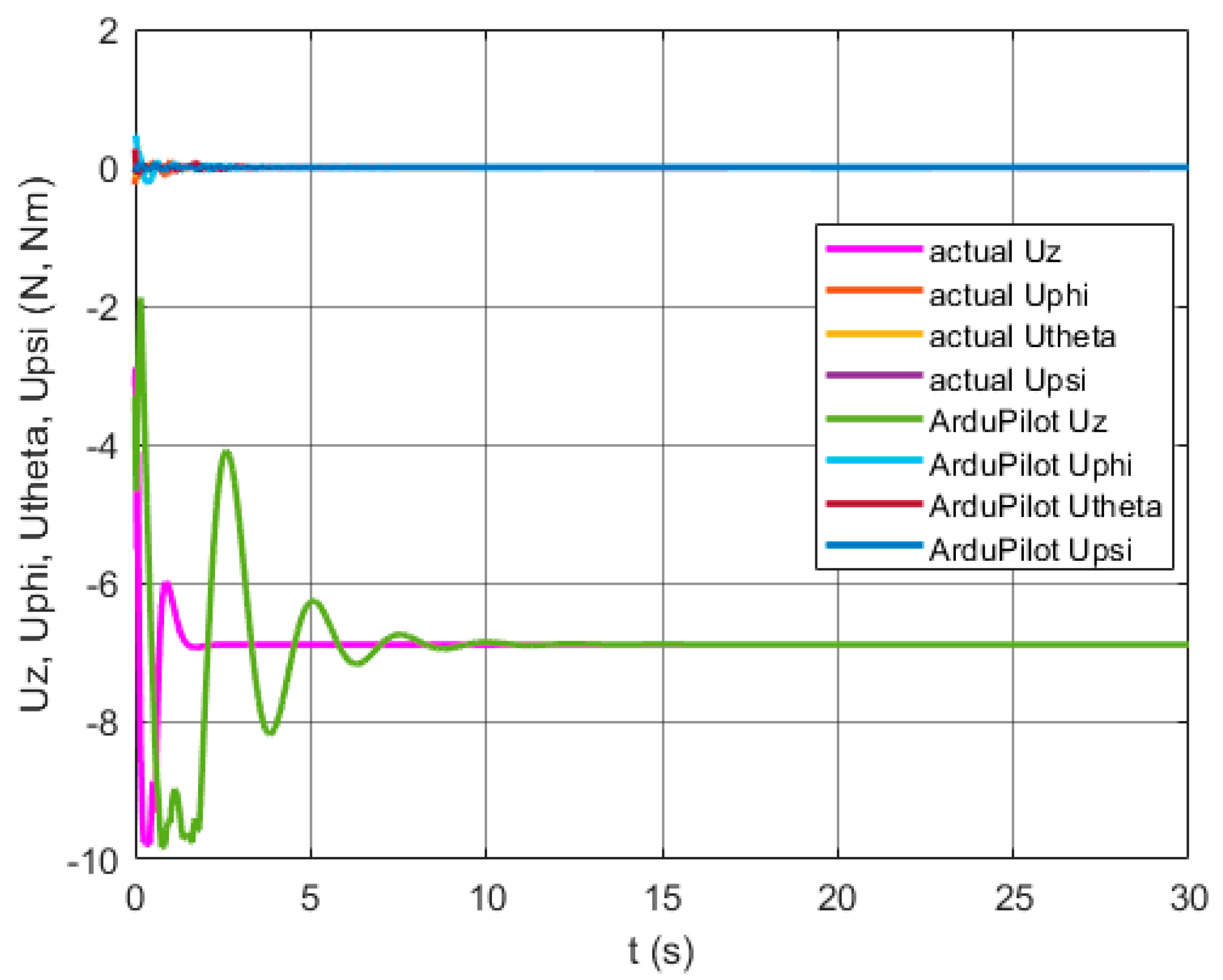
4.5. Vertical Patrol Flight

4.5.1. Desired Trajectory and Conditions of the Experiment

In the next study, a vertical patrol flight was considered. This is a programmed task that can be used, for example, to visually assess the condition of a building [5]. The assumption is that the building has a width of approximately 12 m and a height of 30 m. Once again, a reference trajectory was prepared for the drone to follow, and it was assumed that the UAV could be launched not necessarily precisely at the starting point of the trajectory.

The form of the specified trajectory was determined from the following dependencies [24]:

$$z_d\left(t\right)=0.1t,$$

(33)

$$x_d\left(t\right)=4\sin \left(\frac{2\mathsf{\pi }}{8}t\right),$$

(34)

$$y_d\left(t\right)=4\sin \left(\frac{2\mathsf{\pi }}{8}t\right),$$

(35)

$${\psi }_d\left(t\right)=0.$$

(36)

The weights for the optimization methods are as follows: $w_z=0.4$, $w_x,w_y=0.1$, $w_{\varphi },w_{\theta }=0.$1 and $w_{\psi }=0.2$. To compare the values of the gains obtained using the optimization methods with the gains included in Section 4.3, the same weights were used. By optimizing the PID controller gains for this specific task, the following values were obtained (

Table 5. Controller gains for vertical patrol flight.

Variable	Kp	Ki	Kd
X	11.82	14.55	7.38
Y	13.31	13.68	7.89
Altitude	49.24	104.84	9.33
Roll	2.27	0.01	0.03
Pitch	5.41	9.18	0.16
Yaw	13.08	10.47	0.41

).

4.5.2. Simulation Studies and Summary of the Experiment

The simulation results have been presented in Figure 22, Figure 23, Figure 24, Figure 25, Figure 26, Figure 27, Figure 28, Figure 29 and Figure 30.

Additional constraints for this experiment are the tilt and yaw angles, which, due to the tricopter’s design, are assumed to not exceed the range from −20 degrees to 20 degrees. In the case of the patrol flight motion study, the UAV achieves convergence with the specified trajectory before 1 s has elapsed. From that moment on, the tail angle stabilizes at a pitch of approximately 17 degrees. The object continues to perform a stable flight throughout the simulation, and in the case where the modeled wall was higher, it can be assumed that the UAV would continue to follow the trajectory. In this case, a set of gains from the ArduPilot allowed a satisfactory adjustment measured in the IAE criterion assessment of 6.546 to be achieved. Again, gains selected specifically for the set mission proved to be better, obtaining a quantitative value in the same criterion of 0.896. The main improvement in navigation quality was achieved in the turns of the UAV’s trajectory.

5. Conclusions

The paper describes methods for selecting PID controller gains for controlling the height of a tricopter. A comparison of the IAE criterion shows that each of the four methods used: fmincon, fminimax, lsqnonlin, fminsearch selected better coefficients than the dedicated PID Tuner function [18]. The best function is fminsearch, and for further experiments, this method was used. The regulation was carried out for a larger number of controllers, gradually reaching the control of the tricopter flight, for real tasks that are often performed by unmanned aerial vehicles.

A universal procedure for selecting PID controller gains using optimization methods, which can also be used for other mobile objects, has been presented. The weights were arbitrarily chosen to be able to compare the obtained gains resulting from optimization for both considered trajectories. This highlighted the discrepancies in the optimization of tricopter gains.

The paper demonstrates that by knowing the conditions and trajectory, it is possible to select PID controller coefficients for a specific task using known optimization methods. The optimal coefficients differ depending on the established trajectory, and if the UAV is to be used for a repetitive mission, it is worth selecting specific controller gains for this task. It can also be noted that the UAV does not have to be launched precisely at the starting point of the trajectory, but when planning the trajectory, a reserve of engine power should be left. It is worth selecting weights appropriately for UAV parameters based on experience in flights on the object. The results were compared with analogous experiments obtained for ArduPilot flight controller settings. The settings were downloaded from the controller. Based on the individual simulation experiments, it was shown that better ones can replace the default settings. Updating them from the technical side of the controller only requires connecting it to a computer and saving the new settings. Optimizing the trajectory to the maximum exorbitant results involves operating close to the narrow stability margin. Care must be taken to set boundary conditions well, such as maximum swing angles. As shown, if the planned trajectory is changed, new coefficients should be adjusted so that the stability margin is not exceeded.

This paper can be used by other researchers to select optimal PID controller gains for tricopter objects or by people using other types of UAVs for repetitive, programmed tasks.

References

1. Sanz-Martos, S.; López-Franco, M.D.; Álvarez-García, C.; Granero-Moya, N.; López-Hens, J.M.; Cámara-Anguita, S.; Pancorbo-Hidalgo, P.L.; Comino-Sanz, I.M. Drone Applications for Emergency and Urgent Care: A Systematic Review. Prehospital Disaster Med. 2022, 37, 502–508. [Google Scholar] [CrossRef] [PubMed]
2. Esch, P.V.; Leslie, C. Drones in Facilities Management: Disruptive Innovation to Reduce HSEQ High-Risk Activities. Facil. Perspect. Mag. 2016, 10. Available online: https://www.researchgate.net/publication/304134845_Drones_in_Facilities_Management_Disruptive_Innovation_to_Reduce_HSEQ_High-Risk_Activities (accessed on 17 March 2023).
3. Eschmann, C.; Kuo, C.M.; Kuo, C.H.; Boller, C. Unmanned Aircraft Systems for Remote Building Inspection and Monitoring. In Proceedings of the 6th European Workshop on Structural Health Monitoring, Dresden, Germany, 3–6 July 2012; Available online: https://www.ndt.net/?id=14139 (accessed on 7 March 2023).
4. Vacanas, Y.; Themistocleous, K.; Agapiou, A.; Hadjimitsis, D. Building Information Modelling (BIM) and Unmanned Aerial Vehicle (UAV) Technologies in Infrastructure Construction Project Management and Delay and Disruption Analysis. In Proceedings of the SPIE 9535—Third International Conference on Remote Sensing and Geoinformation of the Environment, 2015, Paphos, Cyprus, 16–19 March 2015. [Google Scholar] [CrossRef]
5. Liang, H.; Lee, S.; Bae, W.; Kim, J.; Seo, S. Towards UAVs in Construction: Advancements, Challenges, and Future Directions for Monitoring and Inspection. Drones 2023, 7, 202. [Google Scholar] [CrossRef]
6. Mohsan, S.A.H.; Othman, N.Q.H.; Li, Y. Unmanned aerial vehicles (UAVs): Practical aspects, applications, open challenges, security issues, and future trends. Intel Serv Robot. 2023, 16, 109–137. [Google Scholar] [CrossRef] [PubMed]
7. Cedro, L.; Wieczorkowski, K. Optimizing PID controller gains to model the performance of a quadcopter. Transp. Res. Procedia 2019, 40, 156–169. [Google Scholar] [CrossRef]
8. Krzysztofik, I.; Koruba, Z. Analysis of Quadcopter Dynamics During Programmed Movement Under External Disturbance. In Nonlinear Dynamics and Control; Lacarbonara, W., Balachandran, B., Ma, J., Machado, J.A.H., Stepan, G., Eds.; Springer: Cham, Switzerland, 2020; pp. 177–185. [Google Scholar] [CrossRef]
9. Abara, D.; Kannan, S.; Lanzon, A. Development and stabilization of a low-cost single-tilt tricopter. IFAC Pap. 2020, 53, 8897–8902. [Google Scholar] [CrossRef]
10. Mahbobur, R.; Mohammad, M.; Assad-Uz-Zaman, M. Design and implementation of a Y-copter: Aerobatic version. AIP Conf. Proc. 2017, 1851, 020089. [Google Scholar] [CrossRef]
11. Shafayat, H.H.; Ariyan, K.; Mazumder, P.; Ahmedullah, A.; Masudul, Q.; Islam, M.; Kanai, S. Design and Development of an Y4 Copter Control System. In Proceedings of the 14th International Conference on Computer Modelling and Simulation, Cambridge, UK, 28–30 March 2012. [Google Scholar] [CrossRef]
12. Kastelan, D.; Konz, M.; Rudolph, J. Fully Actuated Tricopter with Pilot-Supporting Control. IFAC Pap. 2015, 48, 79–84. [Google Scholar] [CrossRef]
13. Sababha, B.; Alzubi, H.; Rawashdeh, O. A rotor-tilt-free tricopter UAV: Design, modelling, and stability control. Int. J. Mechatron. Autom. 2016, 5, 107–113. [Google Scholar] [CrossRef]
14. Abara, D. Modelling, Control and Construction of Tricopter Unmanned Aerial Vehicles. Ph.D. Thesis, The University of Manchester, Manchester, UK, 2022. [Google Scholar]
15. Das, S.; Gouda, G.; Das, A. An Experimental Research on Design and Development of Tricopter. Int. J. Recent Technol. Eng. 2019, 8, 5119–5123. [Google Scholar] [CrossRef]
16. Nam, K.J.; Joung, J.; Har, D. Tri-Copter UAV With Individually Tilted Main Wings for Flight Maneuvers. IEEE Access 2020, 8, 46753–46772. [Google Scholar] [CrossRef]
17. ArduPilot Dev Team, Tricopter Configuration. 2023. Available online: https://ardupilot.org/copter/docs/tricopter.html (accessed on 11 March 2023).
18. Paslier, P. Tricopter. Available online: https://sketchfab.com/3d-models/tricopter-ac47df697aee4834a2b3ff24c83eb180 (accessed on 17 March 2023).
19. Prouty, R.W. Helicopter Performance, Stability and Control; Krieger Publishing Company: Malabar, FL, USA, 1995. [Google Scholar]
20. Dydek, Z.; Annaswamy, A.; Lavretsky, E. Adaptive Control of Quadrotor UAVs: A Design Trade Study with Flight Evaluations. IEEE Trans. Control Syst. Technol. 2013, 21, 1400–1406. [Google Scholar] [CrossRef]
21. MathWorks, Inc. pidTuner. Available online: https://www.mathworks.com/help/control/ref/pidtuner.html (accessed on 7 March 2023).
22. MathWorks, Inc. Optimization Toolbox. 2023. Available online: https://www.mathworks.com/help/optim/ (accessed on 7 March 2023).
23. Jaleeli, N.; VanSlyck, L.S. Nerc’s new control performance standards. IEEE Trans. Power Syst. 1999, 14, 1092–1099. [Google Scholar] [CrossRef]
24. Seif-El-Islam, H.; Latifa, A. Decentralized PID Control by Using GA Optimization Applied to a Quadrotor. J. Autom. Mob. Robot. Intell. Syst. 2018, 12, 33–44. Available online: https://www.jamris.org/index.php/JAMRIS/article/view/460 (accessed on 17 March 2023).
Figure 1. Motor placement in a tricopter [17], where 1, 2, and 3 are the motor numbers, and 4 is the number of the servo controlling the tail angle.
Applsci 13 13118 g001
Figure 2. Tricopter model [18].
Applsci 13 13118 g002
Figure 3. Adopted orientation of the axes [18].
Applsci 13 13118 g003
Figure 4. Block diagram of tricopter altitude control.
Applsci 13 13118 g004
Figure 5. View of the PID tuner.
Applsci 13 13118 g005
Figure 6. The response of the object with all optimization methods compared with the ArduPilot.
Applsci 13 13118 g006
Figure 7. Altitude response.
Applsci 13 13118 g007
Figure 8. Roll angle response.
Applsci 13 13118 g008
Figure 9. Pitch angle response.
Applsci 13 13118 g009
Figure 10. Yaw angle response.
Applsci 13 13118 g010
Figure 11. Control signals.
Applsci 13 13118 g011
Figure 12. Tilt angle response.
Applsci 13 13118 g012
Figure 13. 3D trajectory view.
Applsci 13 13118 g013
Figure 14. X position response.
Applsci 13 13118 g014
Figure 15. Y position response.
Applsci 13 13118 g015
Figure 16. Altitude response.
Applsci 13 13118 g016
Figure 17. Roll angle response.
Applsci 13 13118 g017
Figure 18. Pitch angle response.
Applsci 13 13118 g018
Figure 19. Yaw angle response.
Applsci 13 13118 g019
Figure 20. Control signals.
Applsci 13 13118 g020
Figure 21. Tilt angle response.
Applsci 13 13118 g021
Figure 22. 3D trajectory view.
Applsci 13 13118 g022
Figure 23. X position response.
Applsci 13 13118 g023
Figure 24. Y position response.
Applsci 13 13118 g024
Figure 25. Altitude response.
Applsci 13 13118 g025
Figure 26. Roll angle response.
Applsci 13 13118 g026
Figure 27. Pitch angle response.
Applsci 13 13118 g027
Figure 28. Yaw angle response.
Applsci 13 13118 g028
Figure 29. Control signals.
Applsci 13 13118 g029
Figure 30. Tilt angle response.
Applsci 13 13118 g030