Multi-Physics and Multi-Objective Optimization for Fixing Cubic Fabry–Pérot Cavities Based on Data Learning

Abstract

The Fabry–Pérot (FP) cavity is the essential component of an ultra-stable laser (USL) for gravitational wave detection, which couples multiple physics fields (optical/thermal/mechanical) and requires ultra-high precision. Aiming at the deficiency of the current single physical field optimization, a multi-physics and multi-objective optimization method for fixing the cubic FP cavity based on data learning is proposed in this paper. A multi-physics coupling model for the cubic FP cavity is established and the performance is obtained via finite element analysis. The key performance indices (V, $w_F$, $w_F$) and key design variables (d, l, F) are determined considering the features of the FP cavity. Different data learning models (NN, RSF, KRG) are established and compared based on 49 sets of data acquired by orthogonal experiments, with the results showing that the neural network has the best performance. NSGA-II is adopted as the optimization algorithm, the Pareto optimal front is obtained, and the optimal combination of design variables is finally determined as $\{5,32,250\}$. The performance after optimization proves to be greatly improved, with the displacement under the fixing force and vibration test both decreased by more than 60%. The proposed optimization strategy can help in the design of the FP cavity, and could enlighten other optimization fields as well.

1. Introduction

The high-finesse Fabry–Pérot (FP) cavity is one of the most vital components of ultra-stable lasers (USLs), which have been widely used in several space missions such as LISA (Laser Interferometer Space Antenna) [1], Taiji Program in Space [2], DECIGO (DECI-Hertz Interferometer Gravitational wave Observatory) [3], Post-GRACE (Gravity Recovery and Climate Experiment) [4], etc., as well as in other high-precision fields [5,6,7,8,9,10].

The Pound–Drever–Hall (PDH) method, by which the continuous-wave lasers are locked to the resonance frequency of the FP cavity via high-speed and wide-band electronic control system, is extensively employed in USLs [11,12]. The instability of a laser’s fractional frequency is entirely defined by the length instability of the FP cavity, and perturbations of this length must be minimized to ensure spectral purity [13]. Therefore, the designation of the FP cavity must meet the demand of ultra-high precision coupling in multiple physics fields (optical/thermal/mechanical), including its shape (cylindrical, cubic, spherical, multiple-bore, midplane, etc.), fixing strategy (as small a deformation as possible), and vacuum temperature control (getter and ion pumps, three or more layers of heat shielding, etc.) [14,15,16,17,18].

There have been numerous studies conducted on laser systems, including nonlinear optical materials [19,20] and the design of optical cavities with different shapes [21,22,23,24]. A cubic FP cavity has the advantage of being force-insensitive, making it appropriate for space missions [25]. Based on this idea, follow-up studies have developed several ground-transportable USLs [26]. A typical USL system based on a cubic FP cavity is shown in Figure 1 [27]. An FP cavity made of ultra-low-expansion (ULE) glass is attached to a titanium bracket by four titanium screws, which support the truncated vertices symmetrically. Gaskets made of PEEK are placed between the screws and the spacer for heat and vibration insulation. In the center of the top and bottom surfaces, two mirrors (one planar and one concave) are optically attached. Subsequently, the bracket is affixed to the inner heat shield. Three heat shields employed in all, as depicted in Figure 1b, between which PEEK gaskets are inserted to prevent heat transfer. Finally, the heat shields are secured to the vacuum chamber using titanium screws. The ion and getter pumps maintain a high vacuum level below $2\times {10}^{-6}$ Pa.

As evident from the system composition above, The FP cavity’s performance is significantly affected by the shape parameters of the cavity and the temperature fluctuation. Mechanical simulations have been conducted on cubic FP cavities in many studies, primarily focusing on the static deformation under fixing forces [25] and the variation in performance of different materials [28]. However, as far as we know, there is currently no research that specifically focuses on optimizing the design parameters of the FP cavity in consideration of multi-physics field coupling, which this paper precisely addresses.

The rest of this paper is organized as follows. In Section 2, the multi-physics coupling theory and the finite element method are introduced for problem modelling. The performance results of the cubic FP cavity are thoroughly discussed in Section 3. Section 4 consists of the mechanical optimization process, through which the optimal combination of key design parameters is obtained. Finally, Section 5 presents concluding remarks.

2. Multi-Physics Coupling Theory and Finite Element Method for FP Cavity

2.1. Multi-Physics Coupling Theory

Multi-physical field coupling plays an essential role in understanding and optimizing complex systems involving multiple interactive physical phenomena, helps informed decisions to be reached and making for improved performance and reliability. According to the conservation of energy, the total energy consists of the conductive heat and the radiation heat. The heat conduction equation for the temperature distribution of optical components over time is [29]

$$\rho c\frac{\partial T}{\partial t}=\kappa \left[\frac{{\partial }^{2}T}{\partial x^2}+\frac{{\partial }^{2}T}{\partial y^2}+\frac{{\partial }^{2}T}{\partial z^2}\right]+q_a.$$

(1)

where $\rho$, c, and $\kappa$ are the material density, specific heat capacity, and thermal diffusivity, respectively, t is the time, and $q_a$ is the laser energy absorbed per unit volume. The latter can be represented as

$$q_a(x,y,z,t)=\beta (x,y,z)I(x,y,t),$$

(2)

where $\beta (x,y,z)$ is the volume absorption rate and $I(x,y,t)$ is the distribution of laser intensity

$$I(x,y,t)=P_{0}f(\mathbf{o},\mathbf{e}).$$

(3)

In the above equation, $P_0$ is the beam power and $f(\mathbf{o},\mathbf{e})$ is the distribution of the disposed beam, which is often considered Gaussian:

$$f(\mathbf{o},\mathbf{e})=\frac{1}{2\pi {\sigma }^2}\exp \left(-\frac{d^2}{2{\sigma }^2}\right),d=\frac{\parallel \mathbf{e}\times (\mathbf{x}-\mathbf{o})\parallel }{\parallel \mathbf{e}\parallel }$$

(4)

where $\mathbf{o}$ is the beam origin point, $\mathbf{e}$ is beam orientation, $\mathbf{x}$ is point position, d is the squared distance from the beam axis, and $\sigma$ is the standard deviation.

The laser energy absorbed by the surface is used as the thermal boundary condition, considering the thermal radiation of the surface, yielding

$${\left.\kappa \frac{\partial u(x,y,z,t)}{\partial z}\right|}_{\begin{array}{c}\partial \Omega \end{array}}=\eta I(x,y,t)+ϵ\sigma A(T_{amb}^4-T^4).$$

(5)

We assume that the initial temperature distribution is uniform:

$${\left.u(x,y,z,t)\right|}_{t=0}=T_0,$$

(6)

where $\eta$ is the surface absorptivity, $T_0$ is the initial distribution, $\partial \Omega$ is the boundary of the part, $ϵ$ is the surface emissivity, $\sigma$ is the Stefan–Boltzmann constant, A is the surface area, $T_{amb}$ is the ambient temperature, and T is the temperature of heat radiation sources.

Combining the thermal conduction Equation (1) with the following Equation (7), the deformation of the component can finally be obtained:

$${\nabla }^2\mathbf{u}+\frac{1}{1-2\nu }\nabla (\nabla ·\mathbf{u})=\frac{2(1+\nu )}{1-2\nu }{\alpha }_T\nabla T$$

(7)

where $\mathbf{u}$ is the displacement field, $\nu$ is the Poisson’s ratio, ${\alpha }_T$ is the linear thermal expansion coefficient, T is the internal temperature distribution, and ∇ is the Hamilton operator.

For the purpose of modelling the interaction between different physical fields, we adopted COMSOL multiphysics as the simulation platform [30].

2.2. Finite Element Method and Model Establishment

The finite element method (FEM), which originated in the early 1960s, is by far the most commonly used approach in the numerical analysis and engineering fields [31]. We take a multidimensional steady-state heat conduction process as a model problem, which can be described by the Poisson equation with homogeneous boundary conditions:

$$\begin{array}{c}-{\nabla }^{2}u=f\mathrm{in}\Omega ,\\ u=0\mathrm{on}\partial \Omega ,\end{array}$$

(8)

with domain $\Omega \subset {\mathbb{R}}^d$, where u is the unknown function to be solved and f is the known function (source term). The weak form of Equation (8) can be achieved by choosing a function v from a space U of smooth functions, then forming the inner product of both sides with v, i.e.,

$$-〈{\nabla }^{2}u,v〉=\langle f,v\rangle .$$

(9)

Assume that in addition to having the necessary smoothness, the functions which are to be the solutions satisfy the boundary conditions; the space U of the test functions is of the form $U=\left\{v:v\in C^2(\Omega ),v=0\right.$ on $\left.\partial \Omega \right\}$. More concretely, let d = 2; then, the weak form of Equation (8) is provided by

$${\int \int }_{\Omega }\nabla u·\nabla vdxdy={\int \int }_{\Omega }fvdxdy.$$

(10)

To obtain a numerical method, it is required that U be finite-dimensional with basis $\{u_1,\cdots ,u_n\}$. Then, the approximate solution $u^h$ of Equation (8) can be represented as

$$u^h=\sum _{j=1}^n{c}_j{u}_j.$$

(11)

When a basis has been chosen for the approximation space U, the next step is to determine the coefficients $c_j$ in Equation (11). By inserting $u^h$ into the weak form of Equation (10) and selecting the basis functions of U as the trial functions v, a system of equations

$${\int \int }_{\Omega }\nabla \left[\sum _{j=1}^n{c}_j{u}_j\right]·\nabla u_{i}dxdy={\int \int }_{\Omega }f{u}_{i}dxdy,i=1,\dots ,n$$

(12)

is obtained, which is known as the Ritz–Galerkin method and can be written in matrix form as $Ac=b$, where A is the stiffness matrix

$$A_{i,j}={\int \int }_{\Omega }\nabla u_j·\nabla u_{i}dxdy.$$

(13)

3. Results and Analysis of Multi-Physics Coupling

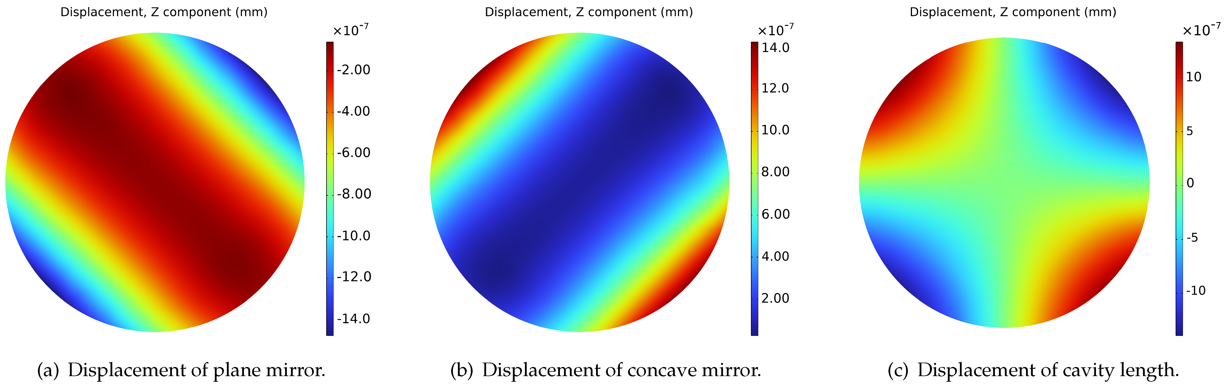
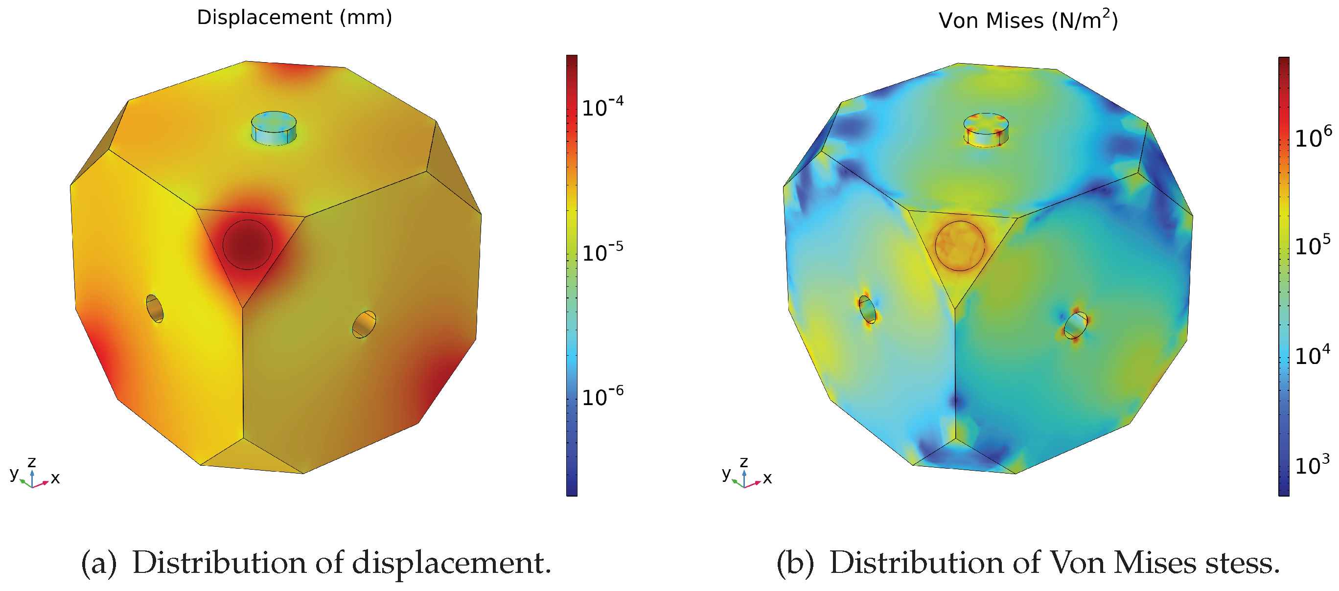
3.1. Displacement Distribution of FP Cavity under the Fixing Force

Taking into account the thermal effect of the laser beam in optical and thermal coupling, the magnitude of the beam power $P_0$ in Equation (3) was set to ${10}^{-4}$ Watt. In thermal and mechanical coupling, the heat radiation to the environment (default 20 °C) and heat conductivity were taken into consideration. In addition, the temperature fluctuation of the vacuum chamber was assumed as ${10}^{-3}$ Kelvin. Then, the finite element model was assigned materials, meshed, and imposed constraints in a solid mechanical analysis. A fixed force of 200 N was applied to each of the four truncated symmetrical vertices. Finally, a virtual prototyping multi-physics coupling model was established and the results were calculated by FEM.

The displacement and Von Mises stress distribution of the FP cavity under the fixing force is shown in Figure 2, with the color map scaled logarithmically for better visualization. It is evident that the displacement and stress amplitude are higher at the four supporting vertices, which have symmetrical distributions as a result of the given fixing strategy. The performance index that should receive the most emphasis is the cavity length change, that is, the displacement of the cavity along the Z axis. Therefore, the Z component displacement of the plane mirror, the concave mirror, and the cavity length change, i.e., the sum of the above two, are shown in Figure 3. It can be seen that the displacement of the two mirrors is symmetrical about the line of 45° and −45°, respectively. In order to further study the variation characteristics of the cavity length change $\Delta L$, two stripe regions of data in Figure 3c with a width of 2 mm along the 45° and −45° were extracted separately. Each consisted of a total of 40,000 data points and was converted to a one-dimensional signal.

Next, a noise-assisted data analysis method called Ensemble Empirical Mode Decomposition (EEMD) is introduced, which consists of an ensemble of workers, each performing Empirical Mode Decomposition (EMD) on a copy of the input signal with added noise. The mean of these EMD results is considered the final result [32]. EMD recursively decomposes a non-stationary signal into data-dependent basis functions termed Intrinsic Mode Functions (IMFs) [33]. In the EEMD process, white noise with a standard deviation of 0.1 is added for the calculation and the number of realizations is set to 100. The EEMD results for the cavity length change along $45°$ and $-45°$ are shown in Figure 4. It can be concluded that the data comprise a fundamental half-sinusoidal component with a low frequency (IMF6) along with other higher-frequency components. The spectral kurtosis (SK) is a common dimensionless time series statistic for detecting and characterizing non-stationarities in a signal that can reflect the random distribution of time series data. A high SK level corresponds to a high level of nonstationary or non-Gaussian behavior [34,35]. The spectral kurtosis of the cavity length change $\Delta L$ along $45°$ and $-45°$ are computed and visualized by kurtograms as shown in Figure 5, for respectively detecting and characterizing the non-stationarities in a signal. The kurtogram uses the normalized frequency, i.e., the sample rate is set to 40,000 Hz for time normalization to 1 s. The kurtograms reveal that the maximum K value is higher in the $-45°$ direction compared to the $45°$ direction, with both directions exhibiting low levels at $K_{max}$, which indicates that the impact of random signal fluctuations with high frequencies is negligible.

3.2. Analysis of Cavity Length Change under the Random Vibration Experiment

During aerospace missions, it is imperative to perform vibration tests on the FP cavity, which is one of the weakest components of a USL.

Table 1. Parameters of the random vibration tests.

Frequency Range/Hz	Power Spectral Density
10~50	3 db/oct (rising slope)
50~300	0.25 g${}^2$/Hz (holding value)
300~2000	−12 db/oct (falling slope)

displays the parameters for random vibration testing using the Long March 5 rocket platform [36]. The test consists of three successive stages: rising, holding, and falling. Moreover, the parameters are more stringent than actual launch conditions to guarantee payload reliability.

The displacement power spectrum densities of the cavity length change responses at different points along the circle of radius 5 mm and 2.5 mm are shown in Figure 6. Various PSD responses along the logarithmic frequency curves at eight points every 45° around the circumference are presented, which first increase, then remain constant, and finally decrease as the test progresses. The PSD value at 180° is the highest, with radius 5 mm, while the lowest value occurs at 315°. By contrast, the PSD values along radius 2.5 mm at 45°, 135°, 225°, and 315° are far more than others (almost zero), which indicates a more complicated $\Delta L$ distribution under the vibration test. Therefore, the parameter of 100 Hz which corresponds to the maximum PSD value of the FP cavity is chosen for the next analysis.

Figure 7 shows the displacement and Von Mises stress distribution under the frequency of 100 Hz, where the color map is logarithmically scaled. Interestingly, the variation of the distribution is non-uniform, i.e., there are local maxima in addition to the four supporting areas, especially on the mirror surface. The Z component displacement of the plane mirror, the concave mirror, and the cavity length change are shown in Figure 8. It can be observed that the cavity length displacement has local maxima and minima around the circumference at 2.5 mm and 5 mm radii. Similarly, two stripe regions of data in Figure 8c with a width of 2 mm along the 45° and −45° were extracted separately and converted to a one-dimensional signal.

The EEMD results of the cavity length change along the $45°$ and −45° directions under the vibration test are shown in Figure 9. In the EEMD process, white noise with a standard deviation of 0.6 is added for the calculation and the number of realizations is set to 200. The IMFs are more complex compared to the fixed force condition’s cavity length change, and additionally suffer from frequency aliasing (IMF3-6). The pattern of the EEMD results is almost identical along both directions, as the two sets of data appear to be highly similar.

The kurtogram of the cavity length change $\Delta l$ data along the $45°$ and $-45°$ directions during the vibration test are respectively computed and visualized in Figure 10. It can be seen that there is a higher maximum K value in the −45° direction compared to the 45° direction, with both directions exhibiting low levels at $K_{max}$, indicating that transient fluctuations of the signal have little influence, even if it appears highly nonstationary.

4. Mechanical Optimization for Fixing a Cubic FP Cavity

4.1. Determination of Design Spaces and Performance Indexes

In Section 3, the variation regularity of the cavity length was calculated and visualized through a multi-physics coupling and signal processing method. The cavity length change is expected to be minimal in all circumstances; consequently, the maximum displacement of the cavity length $w_F$ under the supporting force and the maximum displacement of the cavity length $w_{vib}$ under the random vibration test are determined as performance indexes. In addition, the volume of the cubic cavity V is used as a performance index to ensure a lighter weight.

Apparently, the cavity length change is determined by the mechanical structure. However, there are only a few parameters that can be varied to optimize the cubic FP cavity. As shown in Figure 11, the truncating length of the FP cubic edge l, the diameter of the center hole d, and the magnitude of the supporting force F applied on four vertices are determined as the key design variables.

Considering a reasonable range of the design space in practical engineering, the optimization problem of the FP cavity can be expressed as

$$\begin{array}{cc}\hfill \underset{x}{min}& \hfill O\left(x\right)={[V\left(x\right),w_F\left(x\right),w_{vib}\left(x\right)]}^T\hfill \\ \hfill s.t.& \hfill x_1=d\in [5,13]\mathrm{mm},\hfill \\ \hfill & \hfill x_2=l\in [20,45]\mathrm{mm},\hfill \\ \hfill & \hfill x_3=F\in [100,400]\mathrm{N}.\hfill \end{array}$$

(14)

4.2. Orthogonal Experiments: Design and Implementation

The orthogonal experimental design, which has been widely used in the engineering optimization field [37], is an efficient and economical technique that uses uniform orthogonal combinations of the design parameters to represent the characteristics of the entire design space. For optimization of the FP cavity, an orthogonal experiment containing 49 sets of the design parameters was conducted according to the design space in Equation (14). The corresponding results are shown in

Table 2. Orthogonal experiment design and results.

Number	d/mm	l/mm	F/N	V/m${}^3$ ($\times {10}^{-4}$)	${\mathit{w}}_{\mathit{F}}/$mm ($\times {10}^{-7}$)	${\mathit{w}}_{\mathbf{vib}}$/mm ($\times {10}^{-21}$)
1	5	20	100	9.854	7.842	4.145
2	5	25	200	9.752	14.827	2.064
3	5	30	300	9.601	17.132	5.376
4	5	35	400	9.389	14.815	4.837
5	5	40	150	9.107	3.606	0.132
6	5	45	250	8.746	14.391	1.073
7	5	20	350	9.854	27.447	6.374
8	5	20	200	9.854	15.684	6.743
9	5	25	300	9.752	22.240	0.914
10	5	30	400	9.601	22.843	0.523
11	7	20	400	9.800	40.118	17.790
12	7	25	150	9.699	13.495	0.635
13	7	30	250	9.547	19.568	11.998
14	7	35	350	9.335	17.763	2.962
15	7	40	100	9.054	3.706	2.251
16	7	45	200	8.692	14.024	5.684
17	7	25	300	9.699	26.989	1.270
18	7	35	150	9.335	7.613	3.432
19	7	40	250	9.054	9.265	1.705
20	7	45	350	8.692	24.541	1.662
21	9	20	350	9.730	46.076	10.823
22	9	25	100	9.629	12.392	3.465
23	9	30	200	9.477	21.960	0.461
24	9	35	300	9.265	25.628	8.813
25	9	40	400	8.984	24.200	9.371
26	9	45	150	8.622	13.379	4.828
27	9	30	250	9.477	27.450	4.631
28	9	45	100	8.622	8.919	0.530
29	9	20	150	9.730	19.747	1.841
30	9	25	250	9.629	30.980	3.798
31	11	20	300	9.645	55.853	4.380
32	11	25	400	9.543	70.869	16.213
33	11	30	150	9.391	24.309	5.896
34	11	35	250	9.180	33.908	15.272
35	11	40	350	8.898	37.615	0.556
36	11	45	100	8.536	11.767	0.636
37	11	35	200	9.180	27.126	0.652
38	11	30	350	9.391	56.720	9.568
39	11	35	100	9.180	13.563	4.416
40	11	40	200	8.898	21.494	5.854
41	13	20	250	9.544	62.855	3.054
42	13	25	350	9.442	85.326	21.218
43	13	30	100	9.291	22.917	3.813
44	13	35	200	9.079	42.097	14.350
45	13	40	300	8.797	54.660	0.338
46	13	45	400	8.436	59.989	17.794
47	13	20	400	9.544	100.568	30.596
48	13	40	150	8.797	27.330	0.169
49	13	45	300	8.436	44.992	7.038

.

4.3. Establishment and Comparison of Data Learning Models

In order to establish the nonlinear relationship between the design variables and the performance indexes, the neural network (NN) was initially selected as the fitting model. The working mechanism of a single neuron can be described by

$$h_{\theta }\left(x\right)=g(\sum _{i=1}^n{\omega }_i{x}_i+b),$$

(15)

where $x_i$ is the input of the neural network, b is the bias, $\omega$ represents the corresponding weights, which are the parameters to be learned, and $g(·)$ is the activation function, with sigmoid and ReLU among the most commonly used [38]. A network of neurons organized hierarchically is called a neural network. To minimize the loss function, the gradient descent method was applied through forward propagation and backpropagation as well as through repeated iterations according to the chain rule.

The samples in Table 2 were divided into 90% for training and 10% for testing. The layer size was determined as 40 and Bayesian regulation was adopted as the training algorithm. Figure 12 illustrates the training performance of the neural network model after 1000 epochs. Clearly, the neural network with a very small fitting error (${10}^{-11}$) exhibits excellent performance.

To further compare the performance level of different fitting models, two surrogate models, i.e., the quadratic response surface model and the Kriging model, were selected and established for comparison [37]. The complete quadratic response surface model (RSF) with ten unknown parameters is defined by

$$y_{RSF}\left(x\right)=a_0+\sum _{i=1}^3{a}_i{x}_i+\sum _{j=1}^3{a}_j{x_j}^2+\sum _{i=1}^3\sum _{j=1,j\ne i}^3{a}_{ij}{x}_i{x}_j=\left[1,x,x^2,x_1{x}_2,x_1{x}_3,x_2{x}_3\right]·C,$$

(16)

where $y_{RSF}\left(x\right)$ is the quadratic response surface function, the regression coefficients $a_0$, $a_i$, $a_j$, and $a_{ij}$ are the constant term, the primary term, the quadratic term, the cross terms of the complete quadratic response surface model, respectively, C is the coefficient matrix of the quadratic response surface function, and the response surface coefficients can be fitted using the least squares method.

The Kriging response function $y_{KRG}\left(x\right)$ is comprised of two parts, namely, a regression model and a Gaussian correlation model:

$$y_{KRG}\left(x\right)=\beta f\left(x\right)+z\left(x\right)$$

(17)

where $f\left(x\right)$ is the global basis function, $\beta$ is the regression coefficient, and $z\left(x\right)$ is the Gaussian correlation function, for which the mathematical expectation and covariance are provided by

$$\begin{array}{c}E\left(z\right(x\left)\right)=0\hfill \\ Cov(z\left(x_i\right),z\left(x_j\right))={\sigma }^{2}R(\theta ,x_i,x_j)\hfill \\ R(\theta ,x_i,x_j)={\displaystyle \prod _{d=1}^q}\exp (-{\theta }^d{\left|x_i^d-x_j^d\right|}^{p^d}),\hfill \end{array}$$

(18)

where ${\sigma }^2$ is the variance, $\theta$ is the unknown parameter of association, and $R(\theta ,x_i,x_j)$ is the correlation function of points $x_i$ and $x_j$. For some point x, the predictive value calculated by the Kriging model is

$$\stackrel{\wedge }{y}\left(x\right)=\stackrel{\wedge }{\beta }f\left(x\right)+r^T\left(x\right)R^{-1}(Y-\stackrel{\wedge }{\beta }F),$$

(19)

where $r^T\left(x\right)$ is the covariance matrix between the unknown and known point, Y is the target value matrix of the sample point, and F represents the basis function matrix of the known points.

A test set of five points was used for model validation; the comparison results between the NN and surrogate models are shown in Figure 13. While the three models performed quite well overall, the prediction accuracy of all three models decreases for the volume, displacement under fixing force, and displacement under vibration test. This is likely because the volume variation along the design parameters is the most linear among the three indexes, followed by $w_F$ and lastly $w_{vib}$. As the variation of the index becomes more nonlinear, prediction using the models becomes increasingly challenging.

The root mean square error (RMSE) is adopted as a performance indicator:

$$RMSE=\frac{1}{m{\overline{y}}^{Exp}}\sqrt{\sum _{i=1}^m{(y_i^{Exp}-y_i^{RSM})}^2}$$

(20)

where m is the sample number of the sample training set, $y_i^{Exp}$ is the experiment result, $y_i^{RSM}$ is the prediction at i-th point of response surface model, and ${\overline{y}}^{Exp}$ is the average of experiment points. The fitting accuracy is higher when the RMSE of the fitting model is closer to 0.

The RMSE results of the three prediction models are shown in

Table 3. RMSE comparison of prediction models.

Model	$\mathit{V}/\%$	${\mathit{w}}_{\mathit{F}}/\%$	${\mathit{w}}_{\mathbf{vib}}/\%$
NN	0.12	0.79	2.49
RSF	0.10	1.43	4.76
KRG	0.27	1.56	4.63

. It is evident that the neural network model provides higher accuracy compared to other models, with the KRG model having the largest error. Model performance directly impacts the algorithm’s accuracy when searching for the optimal solution; therefore, the neural network model was used in the next optimization process.

4.4. Evolutionary Algorithm Optimization and Performance Verification

An evolutionary algorithm (EA) is a type of stochastic optimization method inspired by natural processes, especially natural selection in biological evolution; examples include genetic algorithms, particle swarm optimization, ant colony algorithms, and more [39]. EA approaches are used to solve complex optimization and search problems where traditional optimization techniques may struggle. As a typical and proven effective evolutionary algorithm, the Non-Dominated Sorting Genetic Algorithm II [40] (NSGA-II), which uses a fast non-dominated sorting algorithm, sharing, elitism, and crowded comparison, was adopted to search for the optimal combination of design variables.

Specifically, the NSGA-II configuration starts with an initial population of 1000 and uses the previously well-trained NN model to continuously evaluate the population’s performance at each generation. Figure 14 displays the Pareto-optimal front after 100 generations of evolution.

The solution set of the Pareto optimal front surface consists of optimal points that are mutually non-dominant, which means that each point in the Pareto optimal front may be the optimal solution. In most engineering cases, practicality and convenience must be taken into account as well. After subtle selection, the final optimal combination of design variables is determined as $\{5,32,250\}$. The multi-physics model with the optimal parameters was then established and evaluated. A performance comparison showing the results before and after optimization is presented in

Table 4. Performance comparison before and after optimization.

	d/mm	l/mm	F/N	V/m${}^3$$(\times {10}^{-4})$	${\mathit{w}}_{\mathit{F}}/$mm $(\times {10}^{-7})$	${\mathit{w}}_{\mathbf{vib}}/$mm $(\times {10}^{-21})$
Before	10	25	200	9.588	14.858	7.626
After	5	32	250	9.524	5.658	2.852
$\Delta$	$-50\%$	$+28\%$	$+25\%$	$-1\%$	$-62\%$	$-63\%$

. It is satisfying to note that the performance indices are all better than they were before optimization by fine-tune the value and combination of design variables, especially with regard to the displacement under the fixing force and vibration test, both of which are decreased by more than 60%. This ultimate outcome validates the effectiveness of the proposed multi-physics coupling optimization strategy based on data learning.

5. Conclusions

In this paper, a multi-physics and multi-objective optimization strategy for fixing a cubic Fabry–Pérot cavity based on data learning is proposed, consisting of the following three items:

• Performance indices acquired by multi-physics coupling simulation and key design variables determination: a multi-physics model for the cubic FP cavity is established and the performances under fixing force and random vibrations are obtained via finite element analysis, then the key performance indices (V, $w_F$, $w_F$) and key design variables (d, l, F) are determined considering the features of the FP cavity.
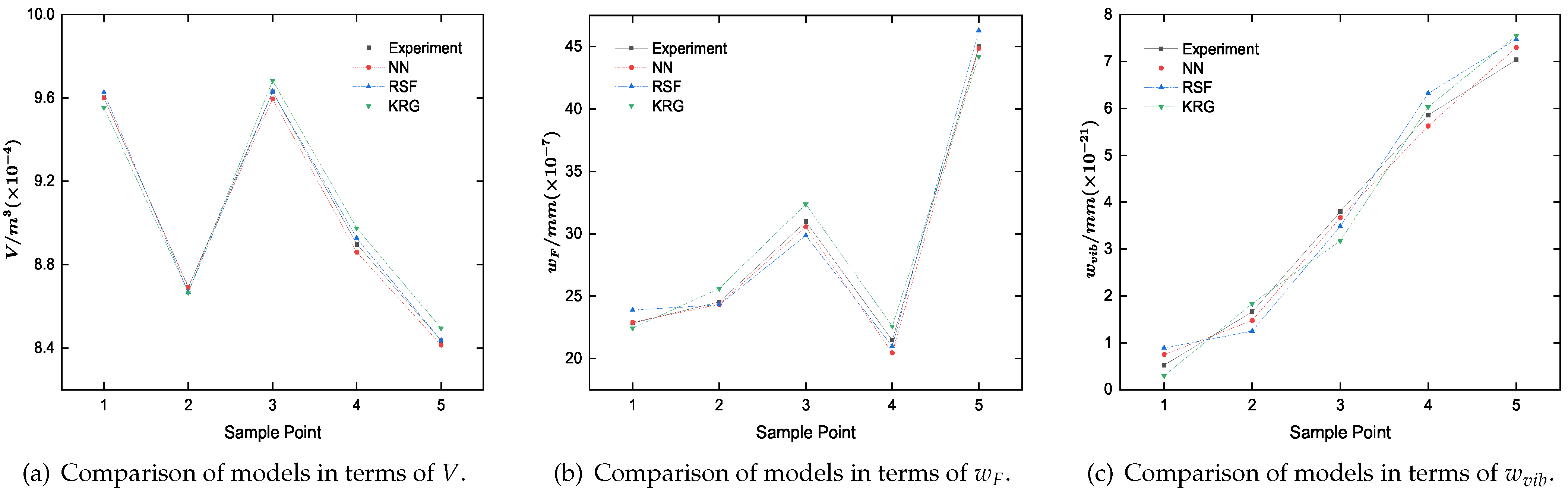
• Training data are obtained by orthogonal experiment and a fitting model is established based on a neural network: 49 sets of data obtained from the orthogonal experiment are used to establish and compare different data learning models (NN, RSF, KRG), with the results indicating that the neural network has the best performance.
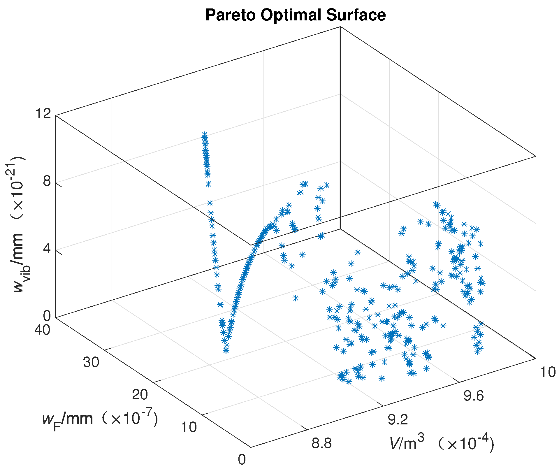
• Finally, an optimized combination of key design variables is obtained using an evolutionary algorithm: NSGA-II is adopted as the optimization algorithm, the Pareto-optimal front is obtained, and the optimal combination of design variables is finally determined as $\{5,32,250\}$. The performance after optimization demonstrates a great improvement, with the displacement under the fixing force and vibration test both decreasing by more than 60%.

In conclusion, the method we have proposed here significantly improves the mechanical performance of the FP cavity and shows great application potential. In the future, we anticipate the application of this optimization strategy in various situations and fields.

References

1. Numata, K.; Anthony, W.Y.; Jiao, H.; Merritt, S.A.; Micalizzi, F.; Fahey, M.E.; Camp, J.B.; Krainak, M.A. Laser system development for the LISA (Laser Interferometer Space Antenna) mission. In Proceedings of the Solid State Lasers XXVIII: Technology and Devices, San Francisco, CA, USA, 2–7 February 2019; SPIE: Bellingham, WA, USA, 2019; Volume 10896, pp. 231–237. [Google Scholar]
2. Luo, Z.; Guo, Z.; Jin, G.; Wu, Y.; Hu, W. A brief analysis to Taiji: Science and technology. Results Phys. 2020, 16, 102918. [Google Scholar] [CrossRef]
3. Cao, S.; Liu, T.; Biesiada, M.; Liu, Y.; Guo, W.; Zhu, Z.H. DECi-hertz Interferometer Gravitational-wave Observatory: Forecast constraints on the cosmic curvature with LSST strong lenses. Astrophys. J. 2022, 926, 214. [Google Scholar] [CrossRef]
4. Flechtner, F.; Morton, P.; Watkins, M.; Webb, F. Status of the GRACE follow-on mission. In Gravity, Geoid and Height Systems: Proceedings of the IAG Symposium GGHS2012, Venice, Italy, 9–12 October 2012; Springer: Cham, Switzerland, 2014; pp. 117–121. [Google Scholar]
5. Acef, O.; Clairon, A.; Du Burck, F. ND:YAG laser frequency stabilized for space applications. In Proceedings of the International Conference on Space Optics—ICSO 2010, Toulouse, France, 30 March–2 April 2004; SPIE: Bellingham, WA, USA, 2019; Volume 10565, pp. 956–961. [Google Scholar]
6. Willke, B.; Danzmann, K.; Frede, M.; King, P.; Kracht, D.; Kwee, P.; Puncken, O.; Savage, R.; Schulz, B.; Seifert, F.; et al. Stabilized lasers for advanced gravitational wave detectors. Class. Quantum Gravity 2008, 25, 114040. [Google Scholar] [CrossRef]
7. Hinkley, N.; Sherman, J.A.; Phillips, N.B.; Schioppo, M.; Lemke, N.D.; Beloy, K.; Pizzocaro, M.; Oates, C.W.; Ludlow, A.D. An atomic clock with 10−18 instability. Science 2013, 341, 1215–1218. [Google Scholar] [CrossRef] [PubMed]
8. Hagemann, C.; Grebing, C.; Lisdat, C.; Falke, S.; Legero, T.; Sterr, U.; Riehle, F.; Martin, M.J.; Ye, J. Ultrastable laser with average fractional frequency drift rate below 5× 10⁻¹⁹/s. Opt. Lett. 2014, 39, 5102–5105. [Google Scholar] [CrossRef] [PubMed]
9. Ushijima, I.; Takamoto, M.; Das, M.; Ohkubo, T.; Katori, H. Cryogenic optical lattice clocks. Nat. Photonics 2015, 9, 185–189. [Google Scholar] [CrossRef]
10. Lucia, U.; Grisolia, G. Time & clocks: A thermodynamic approach. Results Phys. 2020, 16, 102977. [Google Scholar]
11. Black, E.D. An introduction to Pound–Drever–Hall laser frequency stabilization. Am. J. Phys. 2001, 69, 79–87. [Google Scholar] [CrossRef]
12. Guo, X.; Zhang, L.; Liu, J.; Chen, L.; Fan, L.; Xu, G.; Liu, T.; Dong, R.; Zhang, S. An automatic frequency stabilized laser with hertz-level linewidth. Opt. Laser Technol. 2022, 145, 107498. [Google Scholar] [CrossRef]
13. Chen, Q.F.; Nevsky, A.; Cardace, M.; Schiller, S.; Legero, T.; Häfner, S.; Uhde, A.; Sterr, U. A compact, robust, and transportable ultra-stable laser with a fractional frequency instability of 1×10⁻¹⁵. Rev. Sci. Instrum. 2014, 85, 113107. [Google Scholar] [CrossRef]
14. Clivati, C.; Mura, A.; Calonico, D.; Levi, F.; Costanzo, G.A.; Calosso, C.E.; Godone, A. Planar-waveguide external cavity laser stabilization for an optical link with 10−19 frequency stability. IEEE Trans. Ultrason. Ferroelectr. Freq. Control 2011, 58, 2582–2587. [Google Scholar] [CrossRef]
15. Leibrandt, D.R.; Thorpe, M.J.; Notcutt, M.; Drullinger, R.E.; Rosenband, T.; Bergquist, J.C. Spherical reference cavities for frequency stabilization of lasers in non-laboratory environments. Opt. Express 2011, 19, 3471–3482. [Google Scholar] [CrossRef]
16. Argence, B.; Prevost, E.; Lévèque, T.; Le Goff, R.; Bize, S.; Lemonde, P.; Santarelli, G. Prototype of an ultra-stable optical cavity for space applications. Opt. Express 2012, 20, 25409–25420. [Google Scholar] [CrossRef]
17. Pierce, R.; Stephens, M.; Kaptchen, P.; Leitch, J.; Bender, D.; Folkner, W.; Klipstein, W.; Shaddock, D.; Spero, R.; Thompson, R.; et al. Stabilized lasers for space applications: A high TRL optical cavity reference system. In Proceedings of the CLEO: Science and Innovations, San Jose, CA, USA, 6–11 May 2012; Optica Publishing Group: Washington, DC, USA, 2012; pp. 1–2. [Google Scholar]
18. Chen, X.; Jiang, Y.; Li, B.; Yu, H.; Jiang, H.; Wang, T.; Yao, Y.; Ma, L. Laser frequency instability of 6×10⁻¹⁶ using 10-cm-long cavities on a cubic spacer. Chin. Opt. Lett. 2020, 18, 030201. [Google Scholar] [CrossRef]
19. Solnyshkov, D.; Nalitov, A.; Teklu, B.; Franck, L.; Malpuech, G. Spin-dependent Klein tunneling in polariton graphene with photonic spin-orbit interaction. Phys. Rev. B 2016, 93, 085404. [Google Scholar] [CrossRef]
20. Candeloro, A.; Razavian, S.; Piccolini, M.; Teklu, B.; Olivares, S.; Paris, M.G. Quantum probes for the characterization of nonlinear media. Entropy 2021, 23, 1353. [Google Scholar] [CrossRef] [PubMed]
21. Lousteau, J.; Boetti, N.G.; Chiasera, A.; Ferrari, M.; Abrate, S.; Scarciglia, G.; Venturello, A.; Milanese, D. Er3+ and Ce3+ Codoped Tellurite Optical Fiber for Lasers and Amplifiers in the Near-Infrared Wavelength Region: Fabrication, Optical Characterization, and Prospects. IEEE Photonics J. 2012, 4, 194–204. [Google Scholar] [CrossRef]
22. Boetti, N.G.; Pugliese, D.; Ceci-Ginistrelli, E.; Lousteau, J.; Janner, D.; Milanese, D. Highly doped phosphate glass fibers for compact lasers and amplifiers: A review. Appl. Sci. 2017, 7, 1295. [Google Scholar] [CrossRef]
23. Mirza, J.; Ghafoor, S.; Kousar, A.; Kanwal, B.; Qureshi, K.K. Design of a continuous-wave ytterbium-doped tunable fiber laser pump for thulium-doped fiber amplifiers. Arab. J. Sci. Eng. 2022, 47, 3541–3549. [Google Scholar] [CrossRef]
24. Mirza, J.; Ghafoor, S.; Atieh, A.; Kanwal, B.; Qureshi, K.K. Widely tunable and switchable multiwavelength erbium-doped fiber laser based on a single ring cavity. J. Opt. Soc. Am. B 2022, 39, 1118–1129. [Google Scholar] [CrossRef]
25. Webster, S.; Gill, P. Force-insensitive optical cavity. Opt. Lett. 2011, 36, 3572–3574. [Google Scholar] [CrossRef] [PubMed]
26. Jiao, D.; Xu, G.; Gao, J.; Deng, X.; Zang, Q.; Zhang, X.; Liu, T.; Dong, R. A portable sub Hertz ultra-stable laser over 1700 km highway transportation. arXiv 2022, arXiv:2203.11271. [Google Scholar]
27. Zhao, P.; Deng, J.; Xing, C.; Meng, F.; Meng, L.; Xie, Y.; Chen, L.; Liu, T.; Bian, W.; Yin, X.; et al. A spaceborne mounting method for fixing a cubic Fabry–Pérot cavity in ultra-stable lasers. Appl. Sci. 2022, 12, 12763. [Google Scholar] [CrossRef]
28. Wiens, E.; Schiller, S. Simulation of force-insensitive optical cavities in cubic spacers. Appl. Phys. B 2018, 124, 140. [Google Scholar] [CrossRef]
29. Nowacki, W. Thermoelasticity; Elsevier: Amsterdam, The Netherlands, 2013. [Google Scholar]
30. Zimmerman, W. Introduction to COMSOL multiphysics. In Multiphysics Modeling with Finite Element Methods; World Scientific: Singapore, 2006; pp. 1–26. [Google Scholar]
31. Reddy, J.N. Introduction to the Finite Element Method; McGraw-Hill Education: New York, NY, USA, 2019. [Google Scholar]
32. Wu, Z.; Huang, N.E. Ensemble empirical mode decomposition: A noise-assisted data analysis method. Adv. Adapt. Data Anal. 2009, 1, 1–41. [Google Scholar] [CrossRef]
33. Huang, N.E.; Shen, Z.; Long, S.R.; Wu, M.C.; Shih, H.H.; Zheng, Q.; Yen, N.C.; Tung, C.C.; Liu, H.H. The empirical mode decomposition and the Hilbert spectrum for nonlinear and non-stationary time series analysis. Proc. R. Soc. Lond. Ser. A Math. Phys. Eng. Sci. 1998, 454, 903–995. [Google Scholar] [CrossRef]
34. Antoni, J. The spectral kurtosis: A useful tool for characterising non-stationary signals. Mech. Syst. Signal Process. 2006, 20, 282–307. [Google Scholar] [CrossRef]
35. Antoni, J. Fast computation of the kurtogram for the detection of transient faults. Mech. Syst. Signal Process. 2007, 21, 108–124. [Google Scholar] [CrossRef]
36. Meng, L.; Zhao, P.; Meng, F.; Chen, L.; Xie, Y.; Wang, Y.; Bian, W.; Jia, J.; Liu, T.; Zhang, S.; et al. Design and fabrication of a compact, high-performance interference-filter-based external-cavity diode laser for use in the China Space Station. Chin. Opt. Lett. 2022, 20, 021407. [Google Scholar] [CrossRef]
37. Shuiguang, T.; Hang, Z.; Huiqin, L.; Yue, Y.; Jinfu, L.; Feiyun, C. Multi-objective optimization of multistage centrifugal pump based on surrogate model. J. Fluids Eng. 2020, 142, 011101. [Google Scholar] [CrossRef]
38. Sharma, S.; Sharma, S.; Athaiya, A. Activation functions in neural networks. Towards Data Sci. 2017, 6, 310–316. [Google Scholar] [CrossRef]
39. Bartz-Beielstein, T.; Branke, J.; Mehnen, J.; Mersmann, O. Evolutionary algorithms. Wiley Interdiscip. Rev. Data Min. Knowl. Discov. 2014, 4, 178–195. [Google Scholar] [CrossRef]
40. Deb, K.; Pratap, A.; Agarwal, S.; Meyarivan, T. A fast and elitist multiobjective genetic algorithm: NSGA-II. IEEE Trans. Evol. Comput. 2002, 6, 182–197. [Google Scholar] [CrossRef]
Figure 1. USL system based on FP cavity.
Applsci 13 13115 g001
Figure 2. Displacement and Von Mises stress distributions.
Applsci 13 13115 g002
Figure 3. Z component displacement of mirrors under fixing force.
Applsci 13 13115 g003
Figure 4. EEMD results of cavity length change along the 45 ° and −45° directions.
Applsci 13 13115 g004
Figure 5. Kurtogram of cavity length change along the 45 ° and 45 ° directions.
Applsci 13 13115 g005
Figure 6. Displacement power spectrum density of the cavity length change.
Applsci 13 13115 g006
Figure 7. Displacement and Von Mises stress distributions at frequency 100 Hz.
Applsci 13 13115 g007
Figure 8. Z component displacement of mirrors under random vibration test.
Applsci 13 13115 g008
Figure 9. EEMD results for the cavity length change along the 45 ° and −45° directions in the vibration test.
Applsci 13 13115 g009
Figure 10. Kurtogram of the cavity length change along the 45 ° and 45 ° directions under the vibration test.
Applsci 13 13115 g010
Figure 11. Cavity design variables.
Applsci 13 13115 g011
Figure 12. Training results of the neural network.
Applsci 13 13115 g012
Figure 13. Comparison of neural network and surrogate model predictions.
Applsci 13 13115 g013
Figure 14. Pareto optimal surface.
Applsci 13 13115 g014