Article

Studying Corrosion Failure Prediction Models and Methods for Submarine Oil and Gas Transport Pipelines

1
College of Mechanical and Electrical Engineering, China University of Petroleum, Qingdao 266580, China
2
National Engineering Research Center of Marine Geophysical Prospecting and Exploration and Development Equipment, Qingdao 266580, China
3
Offshore Oil Engineering (Qingdao) Co., Ltd., Qingdao 266520, China
*
Author to whom correspondence should be addressed.
Appl. Sci. 2023, 13(23), 12713; https://doi.org/10.3390/app132312713
Submission received: 7 October 2023 / Revised: 22 November 2023 / Accepted: 23 November 2023 / Published: 27 November 2023

Abstract

:
To predict the corrosion failure of carbon steel oil and gas pipelines more accurately, a new corrosion failure prediction model for submarine oil and gas transport pipelines was constructed. A corrosion failure prediction management system was also developed based on the constructed model. To construct the model, corrosion experiments were carried out to analyze the influences of temperature, partial pressure of CO2, pH value, and flow rate acting on the corrosion rate. Based on the analysis results and the corrosion experiment data, a new corrosion failure prediction model containing the time and flow rate for oil and gas pipelines was constructed. The model is based on the existing corrosion prediction model and has a determination coefficient, R2, of 0.9573, which indicates good prediction accuracy. A machine learning prediction model was also used to predict, and the prediction results are compared with that of the proposed model, which further verifies the accuracy and feasibility of the proposed model. A corrosion failure prediction management system for carbon steel oil and gas pipelines was developed based on the constructed model, which makes corrosion failure prediction more convenient and faster and provides a reference for the accurate prediction and efficient control of oil and gas pipeline corrosion failure.

1. Introduction

Carbon steel pipelines are the main facilities for submarine oil and gas transportation. The economic losses and environmental pollution caused by the failure of oil and gas transport pipelines are severe, and corrosion caused by the transportation medium is the main cause of pipeline failure, as shown in Figure 1. Therefore, studying the corrosion failure prediction model and method for submarine oil and gas pipelines is important to the safety of submarine oil and gas transportation.
Until recently, research on the corrosion failure prediction of carbon steel rigid oil and gas pipelines at home and abroad has undergone four stages [1]: an initial empirical model, a semi-empirical model, a mechanism model, and a corrosion failure prediction model established using machine learning algorithms. The initial empirical model was proposed based on experiments and field data [2]. Many improvements have been made since its establishment, such as parameter optimization and making prediction software easier to apply [3,4,5]. However, this type of model cannot be widely used in practice because it does not consider electrochemical reaction kinetics, which increases prediction error. Based on the empirical model, fluid dynamics and other factors must be considered to study the transfer law of corrosive mediums inflow [6]; this is the semi-empirical model. Continuous improvement involves considering the pH value of the medium, corrosion product film, and specific gravity of crude oil for prediction accuracy [7,8]. With the development of computer technology, experts have combined computational methods with experimental and theoretical analysis to reveal the mechanism of corrosion and the established mechanism model. We considered the influence of factors such as the pH value, medium flow rate, and temperature on the reduction reaction of hydrogen ions, water, and oxygen at the cathode and the dissolution process of iron at the anode in the mechanism model [9,10,11,12]. In addition, we propose dimensionless film-forming tendency factors based on the circulation experiment to establish a kinetic model of deposition growth for corrosion product films and better understand the corrosion process [13]. Since data processing has become easier and more efficient, researchers have used machine learning algorithms to analyze experimental or statistical data, building a variety of corrosion prediction models. These algorithms are widely used in numerical modeling and predicting interest fields [14,15,16]. El-Abbasy et al. [17] established a prediction model based on a regression analysis and neural networks [18], where they analyzed the sensitivity of each influencing factor to pipeline corrosion failure. Ossai et al. [19] established a Markov model with non-uniform linear growth in continuous time to predict pit depth distribution after pipeline corrosion. Larin et al. [20] proposed a new algorithm by determining which model of the pipeline’s corrosion area could be established directly. A mechanistic model and an electrochemical model for the carbon dioxide corrosion of mild steel are proposed in [21,22], respectively. Xu et al. [23] conducted failure pressure prediction for pipelines containing corrosion defects based on a DE-BPNN model. However, a predictive model based on machine learning algorithms cannot obtain an explicit reaction formula; it has poor adaptability and requires repeated training. Although the empirical model and semi-empirical model have relational expressions between factors influencing corrosion and corrosion rate, these factors are not fully considered.
Uniform corrosion is the main corrosion form of carbon steel oil and gas pipelines in an acidic solution. We discuss the influence of various factors on uniform corrosion rate in this paper based on carbon steel corrosion simulations and reactor experiments. Considering time and flow rate [24,25], we established a new corrosion prediction model for carbon steel oil and gas pipelines and developed a corrosion prediction management system, providing a reference for the accurate prediction and efficient control of oil and gas pipeline corrosion failures.

2. Corrosion Test

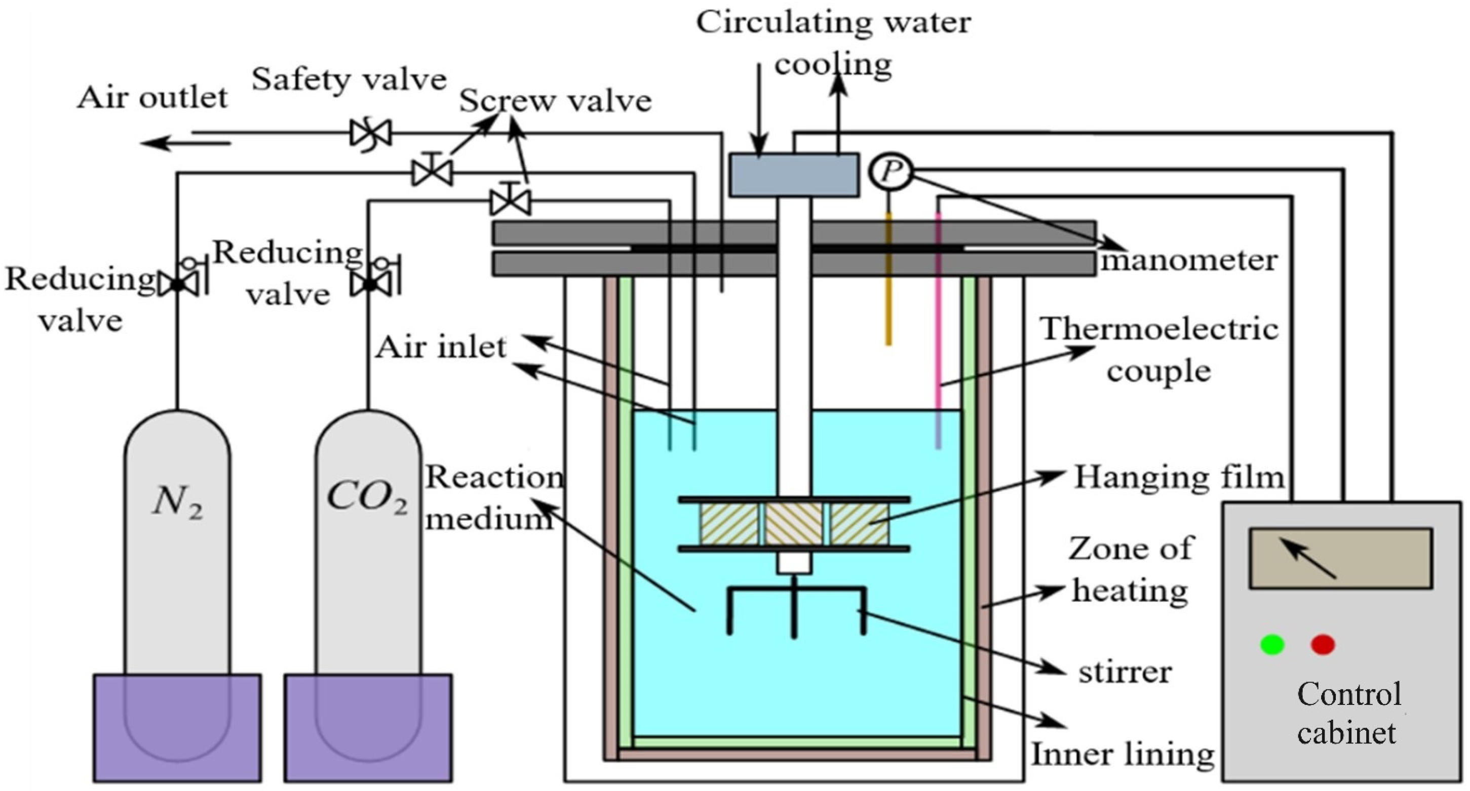
2.1. Arrangement and Experimental Procedure

We applied an FCZ2-10-300 high-temperature and high-pressure reactor to the experiment. The main material of the reactor body was 316 L stainless steel. In order to improve its corrosion resistance, an anti-corrosion lining was added to the innermost layer. The reactor equipment and reactor body are shown in Figure 2a,b, respectively.
The experimental material was X60 pipeline steel, which was made as a corrosion coupon with dimensions of 50 × 10 × 3 mm, as shown in Figure 3. The influence of the partial CO2 pressure, temperature, flow rate, and corrosion time on its corrosion rate was studied next.
The working principle of high-temperature and high-pressure reactor equipment is shown in Figure 4. The temperature in the reactor, stirring speed, and start and stop control of the circulating water pump for the jacket cooling are all controlled by the corresponding knobs on the control cabinet. The pressure in the reactor is displayed by the pressure gauge, which synchronizes with the display screen of the control cabinet.
In this experiment, the corrosion of the experimental material was mainly affected by the CO2 aqueous solution, so the pH value of the solution was only affected by the partial CO2 pressure and temperature. Equation (1) calculates the pH value of a 1 L aqueous solution injected into CO2 [26].
p H C O 2 = 3.82 + 0.00384 T e m 0.51 log ( P C O 2 )
In this formula, pHCO2 is the pH value of the solution under partial CO2 pressure and temperature, Tem (°C) is temperature, and PCO2 (MPa) is the partial CO2 pressure.
We arranged experimental plans using the Response Surface Method [27] according to different experimental requirements. We conducted the experiment, obtained experimental data, and used these data to fit a multivariate function reflecting the relationship between the response and the factor. Finally, we obtained a mathematical model describing the relationship between the experimental factor and the response. When arranging the experimental plans, the axial point of the face-centered cubic design fell on the cube plane but did not exceed the original design level. The estimation of various items was also relatively accurate. In addition, based on the three-level design principle, we used this method to design. We adopted a 1/2 face-centered cubic design and set up 25 groups of experiment plans with a resolution Ⅴ. Table 1 shows the level values of each factor, and Table 2 shows the design and experimental arrangement.
The experiment system was set up to conduct the following experiment arrangements, as shown in Figure 5.
The experimental steps were as follows:
(1)
Sealing test of the reactor. Tighten the bolts three to four times according to the reactor’s loading procedure, and then inject nitrogen into the air inlet to control the pressure in the reactor to a certain value. After 12 h, observe whether the pressure in the reactor decreases. If the pressure remains stable, the reactor seal is effective;
(2)
Proceed with the experiment after confirming the seal. Clean the corrosion coupons using filter papers, and then remove surface grease using absorbent cotton. Finally, immerse the coupons in anhydrous ethanol for further degreasing and dehydration;
(3)
Wrap the coupons in filter paper after cold air drying and put them in the dryer for 1 h to ensure that they are completely dried;
(4)
Prepare the solution. The reactor container has a capacity of 2 L. To ensure safety, the experimental simulation liquid should not exceed 2/3 of the container’s capacity. At the same time, to ensure complete immersion of the coupons in the solution, the simulated solution in this experiment was limited to 1 L;
(5)
Remove the coupons from the dryer. To ensure the accuracy of the experiment, a vernier caliper should be used to measure the size of the coupons with an accuracy of 0.01 mm. Calculate and record the coupons area, weigh the coupons with an accuracy of 0.1 mg, and record the weight as ‘m1’;
(6)
Pour the configured solution into the reactor, then fix the coupons to the clamp of the reactor body. Install and fix the reactor body, open the exhaust port, and inject nitrogen for 1 h to facilitate deoxygenation treatment;
(7)
Tighten the exhaust port after deoxygenation, set the appropriate conditions according to the working conditions, and open the exhaust port when the experimental time is up. Remove the pressure in the reactor, discharge the gas in the reactor, and remove the coupons after cooling;
(8)
Submerge the coupons after the experiment in anhydrous ethanol, and then use absorbent cotton to degrease and remove water. Finally, clean the oxidized sediment on the surface, and then soak the coupons in anhydrous ethanol again. Remove the coupons, wipe them clean, and dry them in the dryer. After drying, record the weighing data (m2), as shown in Figure 6;
(9)
Clean the reactor body and conduct the next set of experiments.
Figure 6. Electronic balance weighing.
Applsci 13 12713 g006

2.2. Experimental Results and Discussion

The uniform corrosion depth can be calculated according to the weighing data before and after the corrosion experiment, namely the surface area and density of the coupons, as shown in Equation (2):
H = 10 Δ W S × ρ
where H (mm) is the uniform corrosion depth; ∆W is poor quality before and after the corrosion experiment, ∆W = m1m2 (g); S (cm2) is the surface area of the coupons; and ρ (g·cm−3) is the density of the corrosion material.
The experiment was conducted following a face-centered cubic design arrangement. The corrosion depth of the coupons under 25 different working conditions is listed in the last column of Table 2. According to the existing literature, the temperature and partial CO2 pressure have the greatest influence on corrosion. Figure 7 shows part of the coupons under experimental conditions for three days, with Tem = 30 °C, 60 °C, and 90 °C; PCO2 = 0.1 MPa, 0.2 MPa, and 0.3 MPa; and Vl = 2 m·s−1.
Figure 7 shows significant local corrosion under the working conditions. The weight loss of the coupons under all experimental working conditions is depicted, as shown in Figure 8.
According to the weight loss recorded in Figure 8, the corrosion rate can be calculated by Equation (3).
v s = 365 × H t
where vs (mm·a−1) is the corrosion rate obtained via the experiment, and t (day) is the corrosion time.

3. Construction of Carbon Steel Corrosion Prediction Model

3.1. Model Establishment

The existing carbon steel corrosion prediction model evolved based on semi-empirical models, as shown in Equation (4) [28].
log R c = 7.545 3359.5 T + 273 2.4622 log ( P C O 2 ) + 5.9977 ( 7 p H C O 2 )
where Rc is the corrosion rate obtained by model.
The shortcoming of this model is that it predicts a fixed corrosion rate, assuming that the corrosion depth is a linear function of time. However, the corrosion morphology continuously evolves throughout the corrosion process, leading to changes in the corresponding corrosion rate. Experiments and simulations demonstrate the impact of the medium flow rate on the pipeline, which cannot be ignored when evaluating the corrosion rate. Therefore, considering time and flow rate, we propose a new corrosion prediction parametric model, as shown in Equation (5).
h = A t b 1 ln ( A ) = b 2 + b 3 T e m + 273.15 + b 4 ln ( P C O 2 ) + b 5 ( 7 p H C O 2 ) + b 6 ln ( V l )
where h (mm) is the remaining thickness of the tube wall, and b1 to b6 are the undetermined coefficients.
The sampling method of the face-centered cubic design cannot be used to simulate the segmental phenomenon caused by temperature adequately. Therefore, only the one-stage model was fitted, which verified the feasibility of the constructed model. These results laid the foundation for developing a more precise segmental corrosion prediction model for carbon steel pipelines. Based on the experimental corrosion data listed in Table 2, the least squares method was used to obtain the undetermined coefficients, as shown in Equation (6).
h = A t 0.14761 A = e ( 5.6126 472.9539 T e m + 273.15 + 0.096 ln ( P C O 2 ) 0.5827 ( 7 p H C O 2 ) 0.0408 ln ( V l ) )
The determination coefficient, R2, of the fitted model is 0.9573, close to “1”, thus indicating the model’s is accuracy. The carbon steel uniform corrosion depth and error curve calculated by this model are shown in Figure 9.
Figure 9a shows that the experimental and simulation values are similar in terms of variation trend and value. In addition, the prediction error curve in Figure 9b shows minimal variation, fluctuating around “0”, with a maximum error of 0.0006. This result confirms the feasibility of the proposed method and accuracy of the fitted model.

3.2. Verification of Prediction Model

To further verify the feasibility and accuracy of the constructed model, BP neural network and random forest regression models based on corrosion data were established for prediction. The BP neural network prediction model was further optimized using the improved particle swarm optimization method based on the prediction results. The prediction results of the established BP neural network prediction model, random forest regression prediction model, and optimized BP neural network prediction model were compared to the prediction model constructed in this paper.

3.2.1. BP (Backpropagation) Neural Network Prediction Model

BP neural networks, also called backpropagation networks, were proposed in the late 1980s, when there was a calculation error lag on the Internet. To improve transmission, it propagates in the opposite direction after reaching the input layer through the calculation [29].
We separated the experimental data into training and test sets according to a certain proportion. If the training set is too small, insufficient training strength is likely to occur. If the training set is too large and the test set is relatively small, the model cannot be verified. Therefore, 80% of the total data was selected as the training set, and the remaining 20% as the test set to build the model. According to the experimental data, five influencing factors were received as inputs, and the uniform corrosion depth of the carbon steel served as output. Therefore, the input layer had five neurons, and the output layer had one neuron. Determining the number of neurons in the hidden layer is crucial to the accuracy of the model, which is calculated according to the following empirical formula:
l = m + n + a
where l is the number of hidden layer neurons; m is the number of neurons in the input layer; n is the number of neurons in the output layer; and a indicates the empirical parameter, 1 ≤ a ≤ 10.
We found that using the BP neural network prediction model achieved better accuracy with nine hidden layer neurons. According to the experimental sample size and desired accuracy, the maximum number of iterations was set to 300, with an expected error of 0.0001 and a learning rate of 0.01.
Due to the inherent randomness in the training process of machine learning algorithms, the results vary each time. In this study, the model was trained 30 times, and the top five results were selected for plotting the predicted corrosion depth of carbon steel and the error curve, as shown in Figure 10.

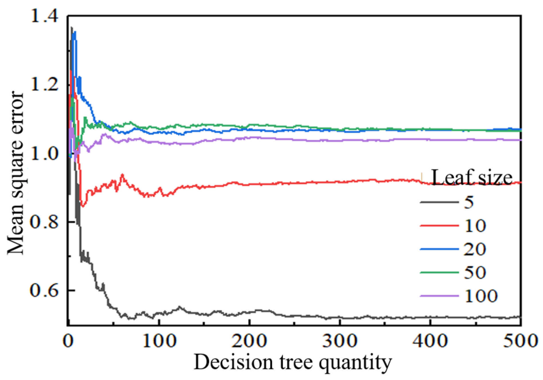
3.2.2. Random Forest Regression Prediction Model

The key parameters affecting the accuracy of the random forest regression prediction model are the leaf size and the number of decision trees. In this paper, the leaf size was set to 5, 10, 20, 50, and 100, and the number of decision trees was set to 200. Figure 11 shows the mean square error of carbon steel corrosion prediction under varying numbers of decision trees and leaf sizes.
Figure 11 shows that errors in prediction models trained using corrosion data are minimized when the leaf size is set to five. According to the fundamental principle of the random forest regression algorithm, the prediction output of the model represents the average predictions from all decision trees. As the number of decision trees increases, the predicted values tend to stabilize. If the decision trees are sequentially built after stability, the computation time will only increase and even lead to “overfitting”. As Figure 11 illustrates, the number of decision trees stabilizes at around 60 for carbon steel corrosion prediction. Based on the analysis, the leaf size was set to five, and the number of decision trees to 60, when the random forest regression corrosion prediction model was established for this paper. If the number of samples is large enough while developing the random forest regression prediction model, the “overfitting” phenomenon will not occur, because the algorithm adopts a back-sampling cross-experiment for verification. If less data are available, dividing the data into training and test sets is necessary. Therefore, 80% of the total experimental data was selected as the training set, while the remaining 20% served as the test set for building the random forest regression corrosion prediction model.
Similar to the BP neural network prediction model, the model underwent 30 training iterations, and the top 5 results were selected for plotting the predicted corrosion depth of carbon steel and the error curve, as shown in Figure 12.

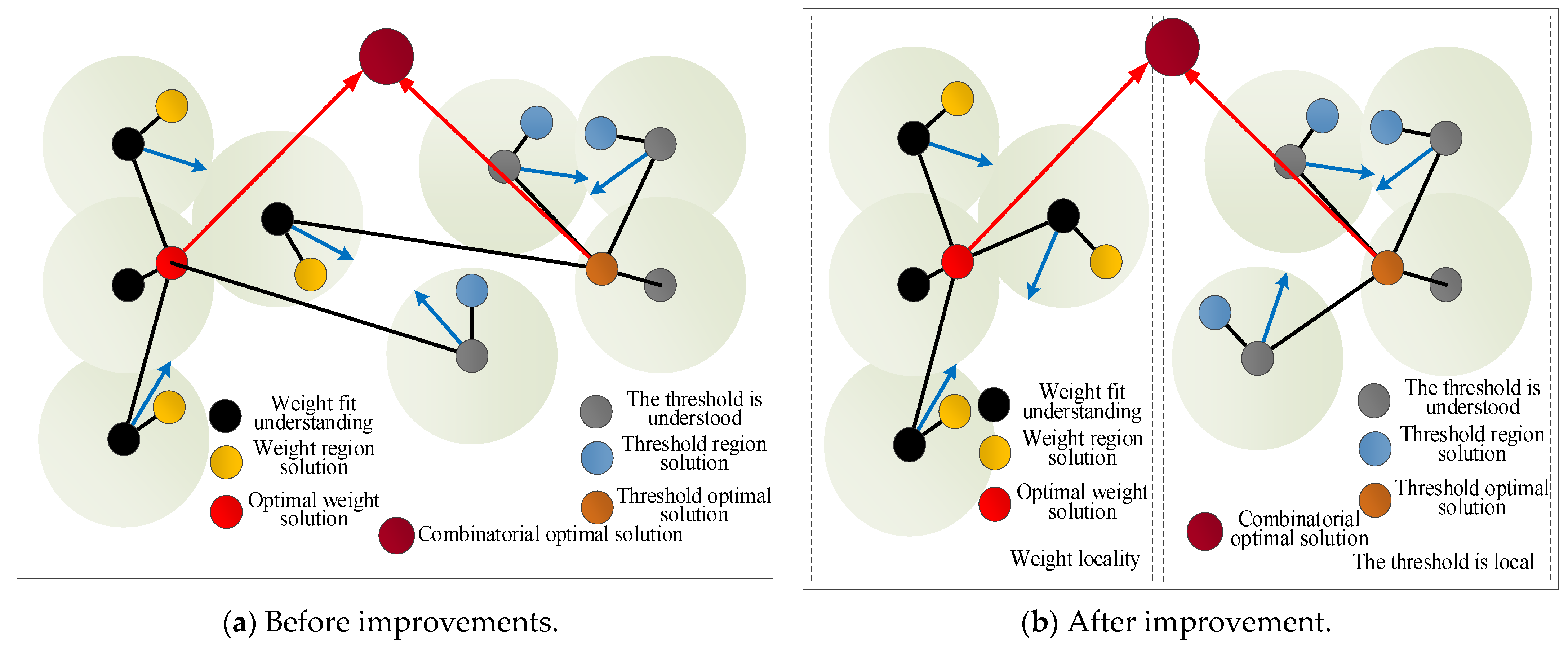
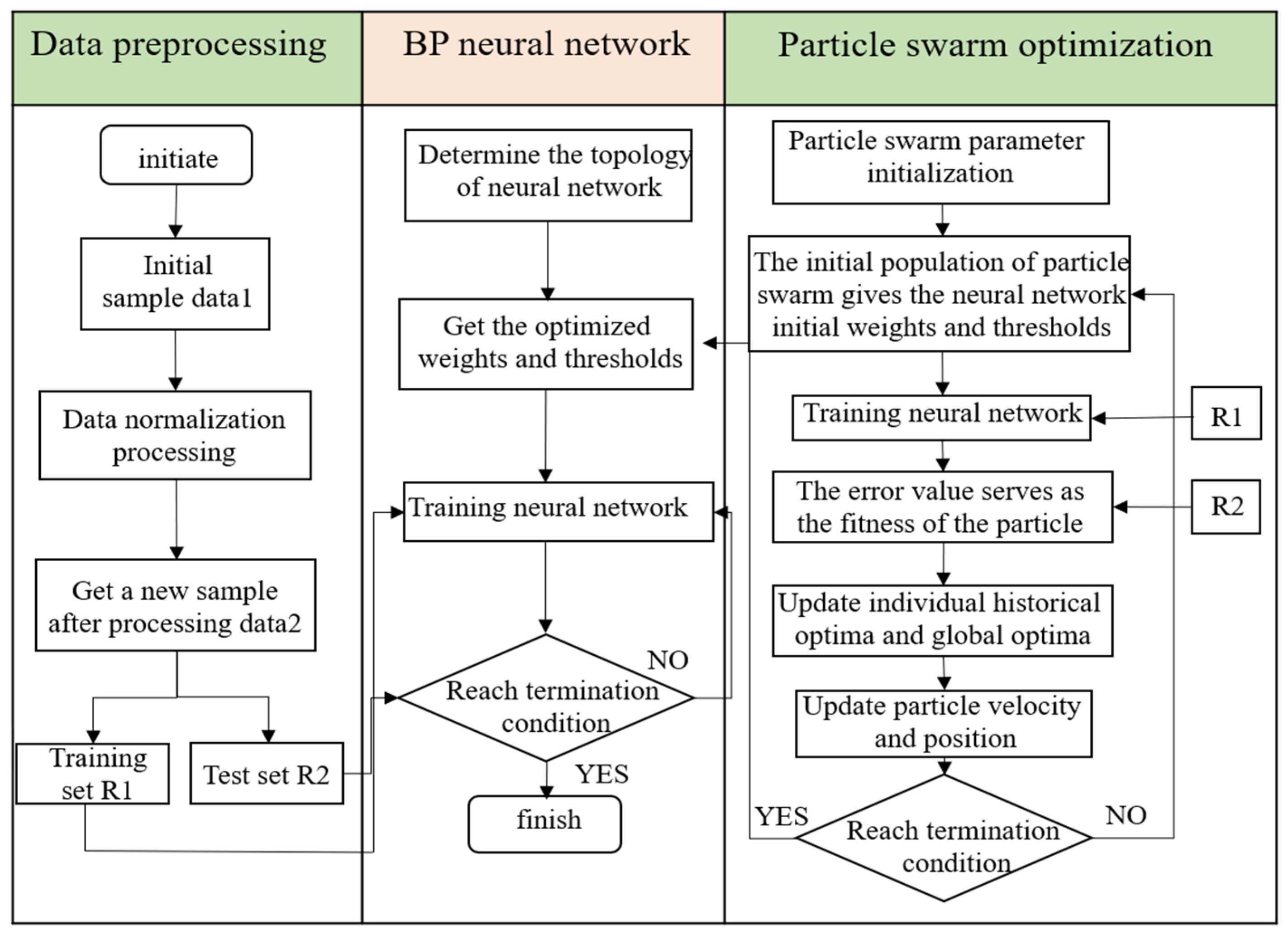
3.2.3. Optimized BP Neural Network Prediction Model

Figure 10 and Figure 12 show that the error of the two machine learning prediction models, the BP neural network model and the random forest regression model, is minor when predicting the corrosion of carbon steel. Nevertheless, the training results of random forest regression predictions are remarkably consistent among the five training runs, whereas those of the BP neural network prediction model exhibit significant variability. This discrepancy is also evident in the error curve charts. The error trend curve of the random forest regression prediction model follows a consistent pattern, whereas the error curve of the BP neural network prediction model appears relatively chaotic. This discrepancy indicates that the random forest regression prediction model demonstrates greater stability, albeit with a marginally higher overall error, whereas the BP neural network model exhibits a lower overall error despite requiring a longer training period. Moreover, the BP neural network prediction model achieves superior accuracy, albeit at the expense of a lengthy optimization process during training. According to the fundamental principles of the BP neural network algorithm, its prediction accuracy hinges significantly on the appropriate tuning of weights and thresholds between layers. The suitability of these values directly impacts training efficiency and the precision of prediction calculations. Therefore, in this paper, we used the enhanced particle swarm optimization algorithm to fine-tune these parameters. According to the principle of the particle swarm optimization algorithm [30,31], the initial position, velocity, particle range, and expected fitness value for single-factor optimization can be iteratively calculated to obtain the optimal value. In this part, the optimization of the two factors, weight and threshold, may be difficult due to the different value ranges of the two factors [32]. Local optimality or long iteration times may occur, as shown in Figure 13a. In light of these challenges, the particle swarm optimization algorithm was refined first. It assigns specific value ranges to the weight and threshold, allowing them to search for optimization within their respective local domains. The mean square error serves as the fitness value, and the combined values of the two factors, which comprise the smallest fitness value, represent the optimal solution, as shown in Figure 13b.
In addition, when the inertia weight factor is introduced into the particle velocity updating formula, the larger the value is, the better the global search effect will be. Otherwise, it will be conducive to local searches. To balance the two situations, the algorithm has a strong global search ability in the early stages of operation, conducts accurate searches after locking the approximate optimal solution range, and introduces dynamic inertia weight factors [33,34]. Its calculation formula is as follows:
w = w s ( w s w e ) ( i m ) 2
where ws is the initial inertia weight, we is the inertia weight when iteration reaches the maximum, i is the current iterations, and m is the total number of iterations.
Generally speaking, when the initial and final inertia weights are 0.9 and 0.4, respectively, the PSO performance is the best. When the progress of iteration shows a parabolic decline, the optimization ability gradually changes from global to local.
The dynamic inertia weight factor is introduced into the velocity update formula of the particle swarm optimization algorithm, as shown in Equation (9).
v i = w × v i + c 1 × r a n d ( ) × ( p b e s t i x i ) + c 2 × r a n d ( ) × ( g b e s t i x i )
where w is the inertia factor; vi is the particle velocity; i = 1,2 … N, N is the total number of particles; c1 and c2 are learning factors that are usually set to 2; and rand() is a random number between 1 and 2.
Figure 14 shows the flowchart of optimization in this model.
We established this model based on the data obtained from a corrosion experiment with a high-temperature and high-pressure reactor. According to the scale of corrosion data, the population size of the particle swarm optimization algorithm was set to 30, the number of iterations was 500, and both c1 and c2 were set to 2. The value range of the neural network weight and threshold was set to [−1, 3.8] and [−1, 8], respectively.
After the parameters were set, the iterative optimization of the particle swarm optimization algorithm was started by reading the carbon steel corrosion data. The iterative weight and threshold parameters were input into the neural network prediction model, and the corrosion of carbon steel materials was predicted again. The training was conducted 30 times, and the prediction curve was drawn based on the top 5 times, as shown in Figure 15.
Figure 15 shows that the five optimal training results of the optimized model exhibit smaller fluctuations, greater stability, and increased accuracy.

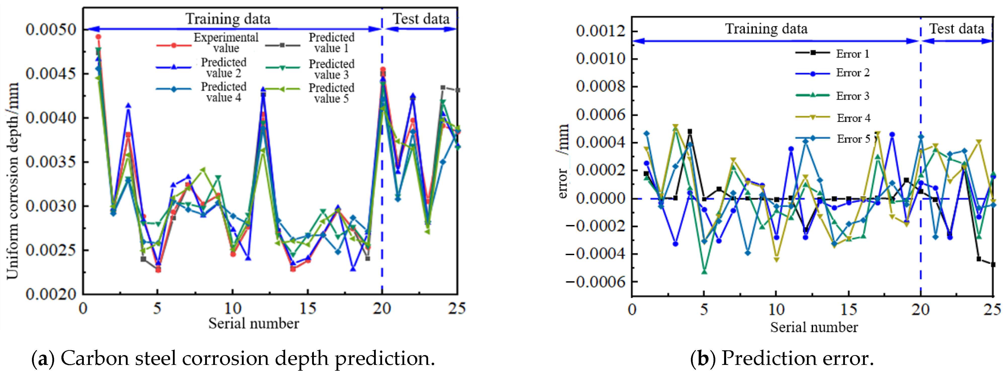
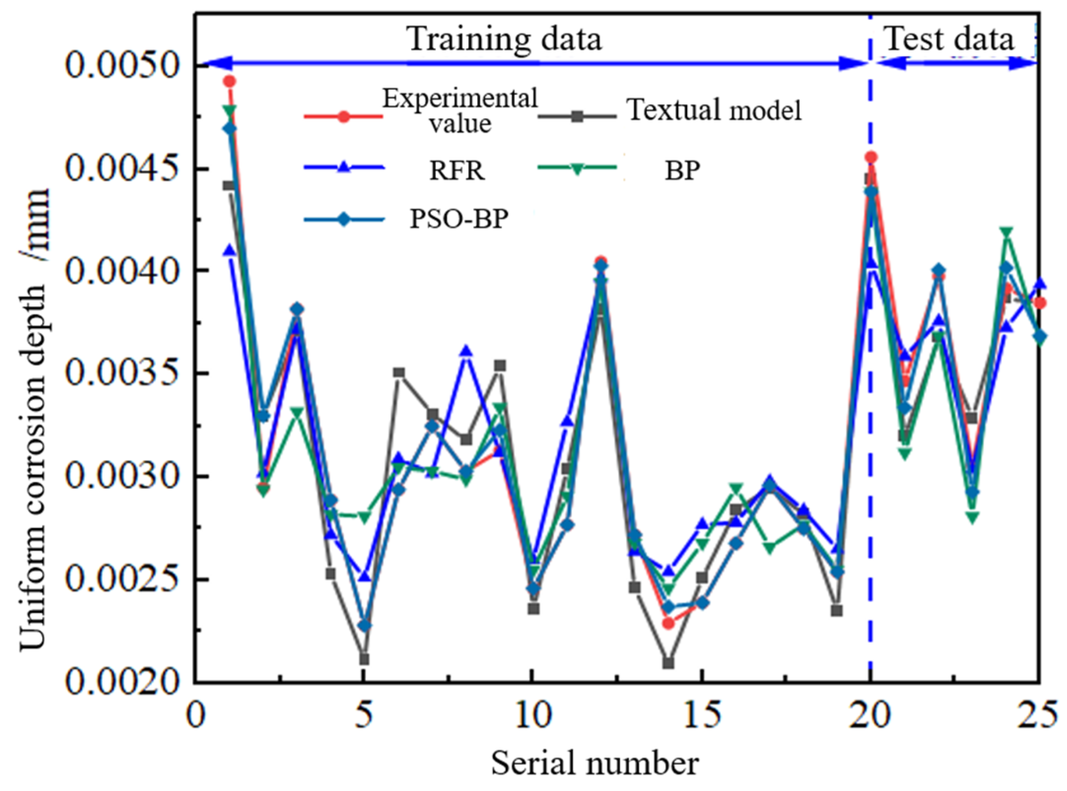
3.2.4. Model Comparison Test

We selected group data with higher accuracy from each established machine learning prediction model and compared them to the model established in this paper. The prediction curves of each model are shown in Figure 16.
Figure 16 shows that the prediction model results are consistent with the prediction trend of the machine learning prediction model. Furthermore, it has high accuracy, so it can be applied to the corrosion prediction of carbon steel materials.

3.3. Management System Development

We developed a corrosion failure prediction management system for carbon steel oil and gas pipelines to broaden the application scope of this model. The main interface of the system is shown in Figure 17.
The model constructed in this paper is integrated and compiled, and so is the parameterized model [35]. Users can import corrosion data and train parameters to improve the model’s prediction accuracy. In addition, our model’s feasibility can be tested by compiling three machine learning algorithm prediction models, namely the BP neural network, random forest regression, and optimized neural network model, into the management system. Users can also use different prediction models to make more convenient and efficient predictions.
As seen in Figure 17, the prediction results of the management system are consistent with Figure 16, proving the feasibility of using the developed management system for prediction. Moreover, the prediction results of the machine learning algorithm are similar to the model described in this paper, thus confirming the accuracy of our prediction model.

3.4. Determination of Corrosion Failure Criteria

At present, according to the oil and gas industry standard SY/T6151 [36], safety parameters affecting carbon steel oil and gas pipeline transportation include the depth of the corrosion pit, the longitudinal length of the corrosion pit, and the circumferential length. We used the maximum depth of the corrosion pit to classify pipelines with different corrosion degrees into five states: light, medium, heavy, severe, and perforated. Table 3 list the parameters.
As seen in Table 3, carbon steel oil and gas pipelines are divided into five corrosion levels, namely five corrosion states, according to the maximum depth of the corrosion pit and wall thickness of oil and gas pipelines. The corrosion state of the pipeline can be determined by calculating the corrosion depth.

4. Conclusions

We arranged 25 orthogonal experiment plans, using face-centered cubic designs derived from the response surface method to improve the shortcomings of existing oil and gas pipeline corrosion prediction models. Corrosion experiments with high-temperature and high-pressure reactors were performed according to experimental arrangements. The corrosion depths of the coupons under different working conditions were obtained. We developed a new corrosion failure prediction model for carbon steel oil and gas pipelines, using the least squares method on corrosion experiment data. This model introduced two variables: time and flow rate. The determination coefficient, R2, of the model was 0.9573, which illustrates a good fitting effect. Three machine learning algorithm prediction models, namely the BP neural network, random forest regression, and optimized neural network, were constructed and compared with the new prediction model proposed in this paper. The prediction model results described in this paper are consistent with the prediction trend of the machine learning prediction models, which had high accuracy, verifying the feasibility and accuracy of the proposed prediction model. Finally, based on the constructed prediction model, we developed a corrosion failure prediction management system for carbon steel oil and gas pipelines, making corrosion prediction for submarine oil and gas transport pipelines more convenient and faster. Based on the uniform corrosion failure prediction model in this paper, the pitting corrosion failure prediction model of the stainless-steel pipeline for oil and gas transmission can be studied further.

Author Contributions

Conceptualization, J.C.; methodology, Z.L.; software, Z.L.; validation, Y.W. and Z.L.; formal analysis, Y.W.; investigation, J.C.; resources, W.X.; data curation, Y.W.; writing—original draft preparation, Y.W. and Z.L.; writing—review and editing, J.C.; visualization, Y.W.; supervision, W.X. All authors have read and agreed to the published version of the manuscript.

Funding

This research was funded by the high-tech ship research project of the Ministry of Industry and Information Technology of the People’s Republic of China (grant no. 2018GXB01-02-003), the Strategic Research and Consulting project of the Chinese Academy of Engineering (grant no. 2022-DFZD-36), and the Fundamental Research Funds for the Central Universities (grant no. 22CX01003A-1).

Institutional Review Board Statement

Not applicable.

Informed Consent Statement

Not applicable.

Data Availability Statement

The data presented in this study are available upon request from the corresponding author. The data are not publicly available due to privacy.

Acknowledgments

We sincerely acknowledge Kuitao Wang and Feng Yin for their administrative and technical support and guidance.

Conflicts of Interest

Author Zhongqi Lu was employed by the company Offshore Oil Engineering (Qingdao) Co., Ltd. The remaining authors declare that this research was conducted without any commercial or financial relationships that could be construed as a potential conflict of interest.

References

  1. Yao, Q.K. Research on Internal Corrosion Prediction Method of Gas Collecting Pipeline in Moxi Gas Field. Master’s Thesis, Southwest Petroleum University, Chengdu, China, 2012. [Google Scholar]
  2. Olsen, S.; Halvorsen, A.M.; Lunde, P.G.; Nyborg, R. CO2 corrosion prediction model—Basic principles. Corrosion 2005, 55, 223. [Google Scholar]
  3. Liu, W.W. Research on CO2 Corrosion Law and Prediction Model of Oil Field Gathering and Transportation Pipeline. Master’s Thesis, China University of Petroleum, Qingdao, China, 2010. [Google Scholar]
  4. Feng, C.Q. Research on CO2 Corrosion Prediction Method and Anti-Corrosion Measure of Gas Well Tubing. Master’s Thesis, Southwest Petroleum University, Chengdu, China, 2015. [Google Scholar]
  5. Sun, Q. Study on CO2 corrosion prediction and anti-corrosion countermeasures of gas well tubing. Pet. Chem. Equip. 2018, 21, 71–74. [Google Scholar]
  6. De, W.C.; Lotz, U. Prediction of CO2 corrosion of carbon steel. Corrosion 1993, 51, 69. [Google Scholar]
  7. de Waard, C.; Lotz, U.; Milliams, D.E. Predictive Model for CO2 Corrosion Engineering in Wet Natural Gas Pipelines. Corrosion 1991, 47, 976–985. [Google Scholar] [CrossRef]
  8. Cui, Y.; Lan, H.Q.; Kang, Z.L.; He, R.Y.; Huang, H.; Lin, N. Improvement of a CO2 corrosion prediction model for natural gas pipelines based on flow field calculation. Acta Pet. Sin. 2013, 34, 386–392. [Google Scholar]
  9. Nešić, S.; Nordsveen, M.; Nyborg, R.; Stangeland, A. A Mechanistic Model for Carbon Dioxide Corrosion of Mild Steel in the Presence of Protective Iron Carbonate Films—Part 2: A Numerical Experiment. Corrosion 2003, 59, 489–497. [Google Scholar] [CrossRef]
  10. Kiani, K.; Shodja, H.M. Response of reinforced concrete structures to macrocell corrosion of reinforcements. Part I: Before propagation of microcracks via an analytical approach. Nucl. Eng. Des. 2011, 241, 4874–4892. [Google Scholar] [CrossRef]
  11. Ožbolt, J.; Oršanić, F.; Balabanić, G.; Kušter, M. Modeling damage in concrete caused by corrosion of reinforcement coupled 3D FE model. Int. J. Fract. 2012, 178, 233–244. [Google Scholar] [CrossRef]
  12. Otieno, M.B.; Beushausen, H.D.; Alexander, M.G. Modelling corrosion propagation in reinforced concrete structures—A critical review. Cem. Concr. Compos. 2010, 33, 240–245. [Google Scholar] [CrossRef]
  13. Nešić, S.; Lee, K.-L.J. A Mechanistic Model for Carbon Dioxide Corrosion of Mild Steel in the Presence of Protective Iron Carbonate Films—Part 3: Film Growth Model. Corrosion 2003, 59, 616–628. [Google Scholar] [CrossRef]
  14. Zhang, Z.M.; Luca, G.D.; Archambault, B.; Chavez, J.; Rice, B. Traffic Dataset for Dynamic Routing Algorithm in Traffic Simulation. J. Artif. Intell. Technol. 2022, 2, 111–122. [Google Scholar] [CrossRef]
  15. Hu, X.; Kuang, Q.; Cai, Q.; Xue, Y.; Zhou, W.; Li, Y. A Coherent Pattern Mining Algorithm Based on All Contiguous Column Bicluster. J. Artif. Intell. Technol. 2022, 2, 80–92. [Google Scholar] [CrossRef]
  16. Jia, Z.; Wang, W.; Zhang, J.; Li, H. Contact high-temperature strain automatic calibration and precision compensation research. J. Artif. Intell. Technol. 2022, 2, 69–76. [Google Scholar]
  17. El-Abbasy, M.S.; Senouci, A.; Zayed, T.; Mirahadi, F.; Parvizsedghy, L. Artificial neural network models for predicting condition of offshore oil and gas pipelines. Autom. Constr. 2014, 45, 50–65. [Google Scholar] [CrossRef]
  18. Du, H.; Du, S.; Li, W. Probabilistic time series forecasting with deep non-linear state space models. CAAI Trans. Intell. Technol. 2022, 8, 3–13. [Google Scholar] [CrossRef]
  19. Ossai, C.I.; Boswell, B.; Davies, I. Markov chain modelling for time evolution of internal pitting corrosion distribution of oil and gas pipelines. Eng. Fail. Anal. 2016, 60, 209–228. [Google Scholar] [CrossRef]
  20. Larin, O.; Barkanov, E.; Vodka, O. Prediction of reliability of the corroded pipeline considering the randomness of corrosion damage and its stochastic growth. Eng. Fail. Anal. 2016, 66, 60–71. [Google Scholar] [CrossRef]
  21. Nordsveen, M.; Nešić, S.; Nyborg, R.; Stangeland, A. A Mechanistic Model for Carbon Dioxide Corrosion of Mild Steel in the Presence of Protective Iron Carbonate Films—Part 1: Theory and Verification. Corrosion 2003, 59, 443–456. [Google Scholar] [CrossRef]
  22. Nesic, S.; Postlethwaite, J.; Olsen, S. An Electrochemical Model for Prediction of Corrosion of Mild Steel in Aqueous Carbon Dioxide Solutions. Corrosion 1996, 52, 280–294. [Google Scholar] [CrossRef]
  23. Xu, L.S.; Ling, X.; Ma, J.J.; Ma, H.Q.; Fu, X.H. Prediction on failure pressure of pipeline containing corrosion defects based on DE-BPNN. J. Saf. Sci. Technol. 2021, 17, 91–96. [Google Scholar]
  24. Kiani, K.; Shodja, H.M. Prediction of the penetrated rust into the microcracks of concrete caused by reinforcement corrosion. Appl. Math. Model. 2011, 35, 2529–2543. [Google Scholar] [CrossRef]
  25. Kiani, K.; Shodja, H.M. Response of reinforced concrete structures to macrocell corrosion of reinforcements. Part II: After propagation of microcracks via a numerical approach. Nucl. Eng. Des. 2012, 242, 7–18. [Google Scholar] [CrossRef]
  26. Zhang, S.C.; Lv, Y.H.; Pei, T.G.; Deng, P.; Chen, B.; Fu, Y.K.; Lai, W.J.; Yao, X.Q.; Lin, X.Z. Failure Analysis of Corrosion and Perforation and Life Prediction of Natural Gas Pipeline. Corros. Prot. 2020, 41, 74–78. [Google Scholar]
  27. Wang, Y.F.; Wang, C.G. Theory and application of response surface method. J. Minzu Univ. China (Nat. Sci. Ed.) 2005, 3, 236–240. [Google Scholar]
  28. Feng, H.Z.; Xing, X.J.; Yan, W. Research on CO2 stage corrosion prediction model for offshore oil casing in China. China Pet. Mach. 2015, 43, 87–92. [Google Scholar]
  29. Chen, J.; Zhao, X.Y.; Cai, L.L.; Zheng, C.; Peng, M. Application of BP neural network in internal corrosion direct assessment methodology for pipelines. Total Corros. Control 2023, 37, 97–102. [Google Scholar]
  30. Zhao, H.; Ma, L. Several rough set models in quotient space. CAAI Trans. Intell. Technol. 2021, 7, 69–80. [Google Scholar] [CrossRef]
  31. Chen, J.; Yu, S.; Wei, W.; Ma, Y. Matrix-based method for solving decision domains of neighbourhood multi-granulation decision-theoretic rough sets. CAAI Trans. Intell. Technol. 2022, 7, 313–327. [Google Scholar] [CrossRef]
  32. Hossein, M.S.; Keivan, K.; Alireza, H. A model for the evolution of concrete deterioration due to reinforcement corrosion. Math. Comput. Model. 2010, 52, 1403–1422. [Google Scholar]
  33. Alhudhaif, A.; Saeed, A.; Imran, T.; Kamran, M.; Alghamdi, A.S.; Aseeri, A.O.; Alsubai, S. A Particle Swarm Optimization Based Deep Learning Model for Vehicle Classification. Comput. Syst. Sci. Eng. 2022, 40, 223–235. [Google Scholar] [CrossRef]
  34. Cao, J. Theory and Method of Emergency Collaborative Decision, 1st ed.; Science Press: Beijing, China, 2015; pp. 32–88. [Google Scholar]
  35. Hsiao, I.; Chung, C.-Y. AI-Infused Semantic Model to Enrich and Expand Programming Question Generation. J. Artif. Intell. Technol. 2022, 2, 47–54. [Google Scholar] [CrossRef]
  36. Hua, C. Contrastive study on new and old evaluation standards of SY/T 6151 for corrosion pipeline. Contemp. Chem. Ind. 2016, 45, 1476–1479. [Google Scholar]
Figure 1. Corrosion of submarine oil and gas transport pipeline.
Applsci 13 12713 g001
Figure 2. High-temperature and high-pressure reactor equipment.
Applsci 13 12713 g002
Figure 3. Size of the corrosion coupon (mm).
Applsci 13 12713 g003
Figure 4. Schematic diagram of a high-temperature and high-pressure reactor.
Applsci 13 12713 g004
Figure 5. High-temperature and high-pressure reactor experimental device.
Applsci 13 12713 g005
Figure 7. Coupons after experiment.
Applsci 13 12713 g007
Figure 8. Weight loss record under 25 different working conditions.
Applsci 13 12713 g008
Figure 9. Predicted corrosion depth of carbon steel and error curve.
Applsci 13 12713 g009
Figure 10. BP neural network model corrosion prediction.
Applsci 13 12713 g010
Figure 11. Parameter selection of random forest regression.
Applsci 13 12713 g011
Figure 12. Corrosion prediction by random forest regression model.
Applsci 13 12713 g012
Figure 13. Optimization schematic diagram of improved pre- and post-particle swarm optimization algorithms.
Applsci 13 12713 g013
Figure 14. Flowchart of optimization model establishment.
Applsci 13 12713 g014
Figure 15. Corrosion prediction of optimized BP neural network model.
Applsci 13 12713 g015
Figure 16. Comparison and prediction test of each model.
Applsci 13 12713 g016
Figure 17. Main interface of oil and gas pipeline corrosion prediction management system.
Applsci 13 12713 g017
Table 1. Level table of experimental factors.
Experimental FactorPCO2 (MPa)Tem (°C)Vl (m·s−1)T (day)
levelLow0.13013
High0.39037
Table 2. Experimental schedule.
Serial NumberOrdinal FactorRespond
PCO2 (MPa)Tem (°C)Vl (m·s−1)t (day)pHCO2H (mm)
10.390374.40.00493
20.260254.50.00295
30.390134.40.00382
40.130174.50.00289
50.130134.50.00228
60.290254.60.00294
70.260154.40.00325
80.330334.20.00303
90.260274.40.00313
100.190134.70.00246
110.230254.30.00277
120.330374.20.00405
130.160254.60.00272
140.130334.50.00229
150.130374.50.00239
160.190174.70.00268
170.260234.40.00296
180.190374.70.00275
190.190334.70.00254
200.390174.40.00456
210.330134.20.00347
220.390334.40.00398
230.260354.50.00306
240.360254.30.00392
250.330174.20.00385
Annotation: H is the uniform corrosion depth.
Table 3. Corrosion failure criteria for carbon steel oil and gas pipelines.
Corrosion ConditionMildModerate SevereExtremely SeverePerforation
Maximum depth of corrosion pit/mm<11~22~50%
Wall thickness
50~80%
Wall thickness
>80%
Wall thickness
Disclaimer/Publisher’s Note: The statements, opinions and data contained in all publications are solely those of the individual author(s) and contributor(s) and not of MDPI and/or the editor(s). MDPI and/or the editor(s) disclaim responsibility for any injury to people or property resulting from any ideas, methods, instructions or products referred to in the content.

