Mineral Characterization Using Scanning Electron Microscopy (SEM): A Review of the Fundamentals, Advancements, and Research Directions

Featured Application

The focus of this review is the use of SEM imaging to gain insight into the composition and morphology of minerals in view of predicting or understanding their reactivity or the process by which they are formed.

Abstract

Scanning electron microscopy (SEM) is a powerful tool in the domains of materials science, mining, and geology owing to its enormous potential to provide unique insight into micro and nanoscale worlds. This comprehensive review discusses the background development of SEM, basic SEM operation, including specimen preparation and image processing, and the fundamental theoretical calculations underlying SEM operation. It provides a foundational understanding for engineers and scientists who have never had a chance to dig in depth into SEM, contributing to their understanding of the workings and development of this robust analytical technique. The present review covers how SEM serves as a crucial tool in mineral characterization, with specific discussion on the workings and research fronts of SEM-EDX, SEM-AM, SEM-MLA, and QEMSCAN. With automation gaining pace in the development of all spheres of technology, understanding the uncertainties in SEM measurements is very important. The constraints in mineral phase identification by EDS spectra and sample preparation are conferred. In the end, future research directions for SEM are analyzed with the possible incorporation of machine learning, deep learning, and artificial intelligence tools to automate the process of mineral identification, quantification, and efficient communication with researchers so that the robustness and objectivity of the analytical process can be improved and the analysis time and involved costs can be reduced. This review also discusses the idea of integrating robotics with SEM to make the equipment portable so that further mineral characterization insight can be gained not only on Earth but also on other terrestrial grounds.

1. Introduction

The rapid pace of technological development requires a detailed study of minerals to a further extent to meet the unprecedented material demands of the evolving world. There are more than 5956 species of minerals known today, and the number of new identifications is evolving, with as many as 50 new types identified each year [1,2]. Quantitative measurements and qualitative analyses of mineral compositions within mining ores and reservoirs have valuable importance with practical applications. Comprehensive and accurate information can be gathered for the identification of rocks and minerals, including structural characteristics and mineral composition, which can provide worthy information about pore structure and reservoir heterogeneity [3,4,5].

The qualitative analysis of minerals is usually conducted through conventional optical microscopy (OM), also known as light microscopy (LM), scanning electron microscopy (SEM), and infrared spectroscopy methods [6,7,8]. Mineral characteristics and mutual relationships are broadly analyzed by OM; however, due to resolution limitations, qualitative analyses of micro and nanoscale particles, including their structural characteristics and mineral morphology, are lacking [9,10]. OM can obtain a maximum useful magnification of 1000 times [11]. The wavelength of imaging radiation can be further decreased for better resolution (i.e., higher useful magnification). OM uses light as imaging radiation, while electron microscopy makes use of electrons to magnify the specimen. Electron beams are accelerated with high energies (from 2 keV to 1000 keV, representing smaller wavelengths of 0.027 nm to 0.0009 nm) in electron microscopes [11].

The bombardment of high-energy electron beams on the atoms in a specimen can result in various possible interactions (Figure 1), which are subject to the thickness of the specimen. The electrons can be transmitted unabsorbed through the specimen if its thickness is very small and can be used to form an image in transmission electron microscopy (TEM) [12]. In contrast, with thicker specimens, electrons are not transmitted, and the particles (electrons, photons, X-rays, etc.) emerging from the surface of the specimen provide morphological and structural information. Low-energy electron beams ranging from 0.1 keV to 30 keV penetrate the sample from a few to tens of nanometers. Medium-energy beams ranging from 30 keV to 1000 keV penetrate from tens of nanometers to micrometers, while high-energy beams, which are usually above 10,000 keV, can penetrate from several micrometers to millimeters within samples. The retrieved information signals are used in SEM to provide sample characteristic information [13].

SEM can be used to analyze the crystalline structure, surface topography, electrical behavior, and chemical composition of approximately 1 µm of the top part of a specimen [11]. The behavior of the specimen under several conditions can be investigated using SEM, as a variety of specialized stages can be applied, such as cold [14], hot [15], or in situ mechanical testing [16]. For instance, cathodoluminescence (emission of light) works very well for temperatures near absolute zero compared to room temperature [17,18]. The images formed are much less noisy from light emitted by a cold specimen. For similar reasons, transmission electron microscopy is used for samples cooled to cryogenic temperatures and is known as cryogenic electron microscopy (Cryo-EM) [19,20,21].

SEM has additional advantages over OM. For example, SEM has a powerful useful magnification of 1,000,000 times and can reach the nanometer scale [22]. This allows an in-depth examination of the specimen compared to OM. Surface smoothness affects the quality of micrographs taken with OM, as high-magnification OM possesses a very low depth of field. SEM, on the other hand, has a large depth of field that benefits simultaneous focus on the specimen surface, irrespective of surface roughness [23]. SEM has the possibility to go beyond analyzing the surface topography [24], providing information about the chemical composition [25], crystal structure [26], and electrical properties [27]. Confidence in the analysis can be further gained by switching between different imaging techniques, which enables cross-correlation of the acquired information. SEM is also beneficial over TEM in several analytical scenarios. SEM can cater to larger-sized samples (wafers of 200 mm diameter, while specially adapted SEMs can go further up), in comparison to TEM, which can analyze to only 2.3 mm or 3 mm [22]. SEM is a nondestructive analytical technique [28], while the specimen preparation process of TEM makes it a destructive technique [29]. The time needed for preparing the sample for SEM is also less when compared to the TEM technique.

SEM can be further classified into three types, i.e., conventional SEM (CSEM), low vacuum SEM (LVSEM), and environmental SEM (ESEM) [30,31,32]. CSEM usually possesses a high vacuum (10⁻⁶ Torr) condition for interaction of the electron beam and specimen. This allows the emission of low-energy secondary electrons from the specimen, resulting in minimum collisions with gas molecules present in the chamber. CSEM reinforces those analyses where dehydration and cracking of the sample (due to high vacuum) is not a problem, such as the identification of alkali–silica reactivity in concrete [33]. The second type, LVSEM, is similar to CSEM, with adaptation of elevated pressure (0.2 to 1 Torr) operations as well. The LVSEM environment slowly dissipates any liquid water present in the sample; therefore, crack propagation in the sample moves very slowly. For nonconductive samples, it is important to add a conductive coating to avoid any charging effects. The third type, ESEM, permits imaging of the sample at high humidity and therefore is considered “wet mode.” ESEM has a relatively high-pressure environment, i.e., 0.2 to 20 Torr, which reduces or eliminates dehydration. The elevated pressure reinforces the ionization of gas molecules due to the emission of surface charges, thereby reducing the need for conductive coatings [34]. The strength of the electron signal increases with the ionization of gas molecules, providing better results. ESEM supports coherent imaging but has limited ability in X-ray microanalysis, as frequent collisions lead to defocusing and scattering of the electron beam, which makes the position of the beam on the specimen uncertain. Field emission gun SEM (FEG SEM) typically falls under the category of CSEM, as its operation includes high vacuum conditions. In conclusion, the type of SEM should be chosen based on the nature of the specimen and the needed analysis.

1.1. Background Development of SEM

The idea of using electron microscopy dates back to the previous century when Ruska and Knoll conducted their experiments in 1932 [35,36]. This instrument was named the transmission electron microscope (TEM), based on its working principle and application, in which electrons were transmitted through thin specimens to magnify beyond the levels of optical microscopes of that time. In 1938, a scanning coil was added to TEM by Von Ardenne, introducing the era of scanning transmission electron microscopy (STEM) [37,38]. It provided a magnification of 8000× with a resolution of 50–100 nm at 23 keV. Ardene developed a laboratory instrument with various features, which became the standard for developing and inventing new SEM systems [39]. A new explanation of SEM for analyzing thick samples was presented by Zworykin, Hillier, and Snyder in 1942. It was found that the emission of secondary electrons can be used for topographic contrast. Oatley and McMullan developed the electrostatic lens for SEM in 1952. Smith understood the role of signal processing in improving SEM micrographs and laid the foundation for nonlinear signal amplification. Another contribution from Smith was the production of double deflection scanning for upgrading the scanning system [39]. Wells designed a new stereoscopic pair for investigating the third dimension in SEM micrographs in 1953. The work of Everhart and Thornley indicated the development of a secondary detector, which served as a tool for improving the signal-to-noise ratio and overall increasing the collected signals. Pease used three magnetic lenses in building the SEM V system, which is considered the first commercial SEM instrument available, under the name “Stereoscan” Cambridge Scientific Instruments Mark 1 in 1965 [40]. Since then, several advancements have been made to improve SEM analysis, such as upgrading electron source for better electron emission, resulting in efficient and clear SEM resolution. Another beneficial advancement in SEM development pertains to the invention of an energy-dispersive spectrometer (EDS). The system has been used in conjunction with SEM since 1968 and makes use of solid-state detectors for measuring X-rays [39]. SEM has been developing with the advent of modern equipment. Danilatos studied the effect of the environment on analyzed samples during 1991–1993, which led to the development of an environmental scanning electron microscope (ESEM) for examining the surface of a specimen, whether it is dry or wet [41,42]. Among these advancements in SEM, the most recent is the generation of digital images, which are then displayed on computers for analysis. At present, the majority of SEM instruments have modern software for analyzing the obtained data and EDS systems, which make use of computer programming for evaluating the composition of various elements present in the sample [39]. The use of modern software provides improved quantitative analysis and converts the X-ray intensity into the chemical composition of the sample in a relatively shorter period of time.

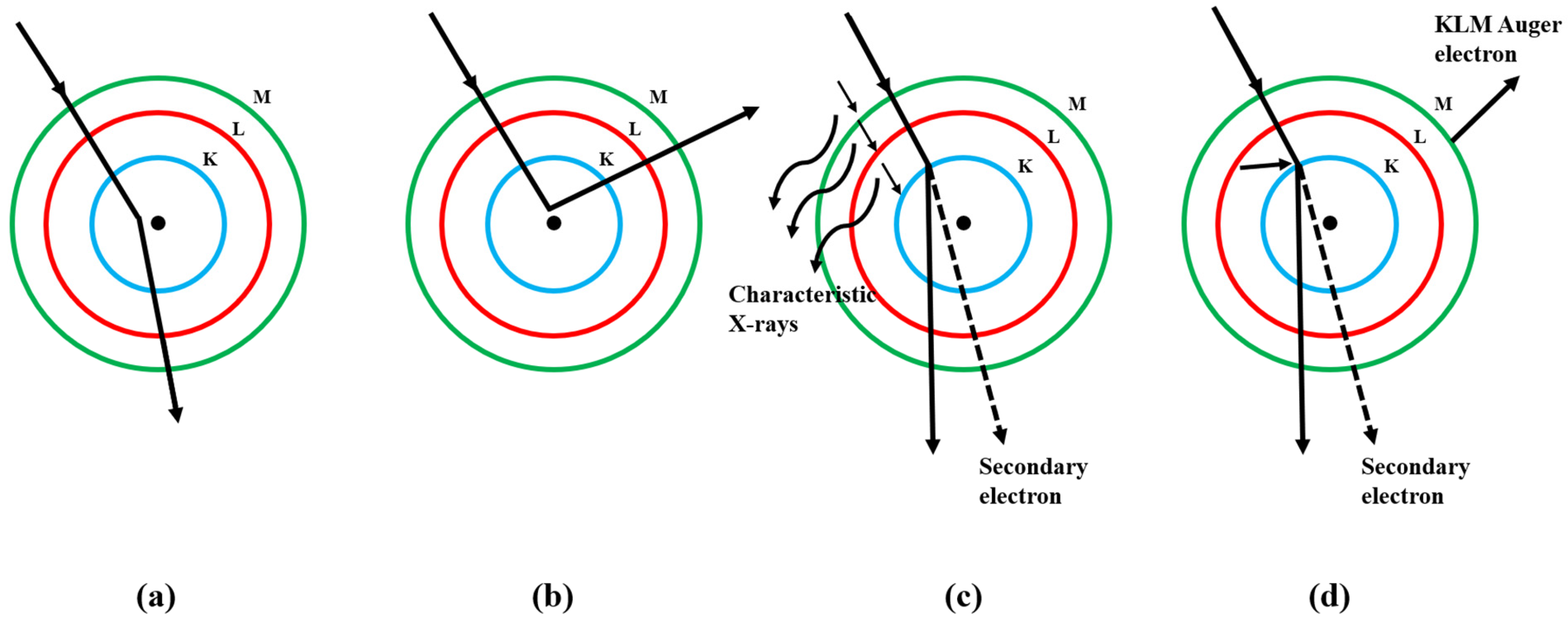
1.2. Basic SEM Operation

The typical energies of incident electrons originating from electron guns in SEM generally range from 2 keV to 40 keV [11]. SEM instruments can be classified based on the range of energy, which is subject to the type and nature of the sample and analysis, such as low voltage SEM, standard SEM, high-resolution SEM, and field emission SEM. Electron guns are also chosen based on the intended application, and three types of electron guns are usually used for SEM. Type one is the tungsten filament electron gun, which is heated over 2500 °C, resulting in the thermal emission of electrons from its tip [43,44]. The second type of electron gun is the lanthanum hexaboride filament, which produces thermionic emissions, with the advantages of a longer working life and brighter beam of electrons from a larger maximum beam current [45,46]. These electron guns are relatively more expensive than conventional tungsten filament guns. Field emission guns are the third type of electron gun and are known as cold cathode electron emitters, as heating is not involved in the process [47,48]. It works with the application of a very high electric field to a finely pointed tip, which results in providing the brightest beam with a very small deviation in electron energy. Since field emission guns need 10⁻¹⁰ Torr of pressure to preserve the tip, the cost of SEM with these guns becomes high [11].

The electron beam is demagnified into a fine probe by two or three electromagnetic condenser lenses. Scan coils are used with fine probes for scanning across the selected surface area of the specimen. The electrons originating from the probe penetrate into the sample in a teardrop-shaped volume (Figure 2). The overall dimensions of this volume are determined by various factors, such as the electron beam energy and atomic masses of the constituent elements present in the specimen. Higher energy and lighter atomic masses of elements tend to result in increased penetration depth inside the sample. The angle of incidence does not significantly affect the penetration depth; rather, it affects the angle of deflection, scattering, and other electron interactions as the beam traverses through the specimen. The production of secondary, Auger, and backscattered electrons takes place due to the interaction of the electron beam with the sample surface. It also accompanies the production of characteristic, continuum, and fluorescent X-rays (Figure 2).

Elastic interaction between an electron beam and the sample results in electrons reflecting back, termed backscattered electrons (Figure 2). These electrons are used for generating high-resolution images of the constituent elements present in the specimen. Inelastic collisions result in relatively lower energy electrons originating from the atoms of the sample, which are known as secondary electrons and are helpful in investigating the topography of the specimen surface. Auger electrons are emitted when excited atoms release energy and are characteristic of the sample elements. These electrons help in understanding the elemental composition of the specimen. When the electron beam displaces an electron from the inner shell of an atom, another electron from a higher valence shell takes its place, resulting in a small loss of energy in the form of an X-ray photon. It is considered a characteristic X-ray and helps in investigating the particular element from which it is emitted. The electrostatic force experienced by the high-energy incident electron beam due to the presence of atomic nuclei results in deflections/accelerations/decelerations of electrons. This results in the production of continuum X-rays (also known as Bremsstrahlung or Brems X-rays), with a continuous spectrum ranging from low to high energies (Figure 2). Continuum X-rays do not contribute to primary elemental analysis; however, they help in studying the interaction between the sample and the electron beam. Fluorescent X-rays are a subset of characteristic X-rays, resulting from the filling up of the inner shell by outer shell electrons (Figure 2). Characteristic X-rays are emitted from the vacancy left by an ejected inner shell electron, while fluorescent X-rays are produced when the outer shell electron fills the vacancy. Fluorescent X-rays contribute valuable elemental information in addition to that provided by the main characteristic X-rays. They also help in studying the background radiation in the X-ray spectrum [11] (Figure 1).

The signals of electron and X-ray production are collected by various detectors present in the specimen chamber of the SEM. A monitor is fed with the signals from each detector, and a rectangular pattern of parallel scanning lines is synchronized with the electron beam [11]. Field emission gun SEM (FEG-SEM) can produce high-resolution secondary electron images owing to the intense electron beam and is capable of achieving subnanometer to nanometer-scale resolution [49].

It is important to understand the meaning of the magnification value in SEM images. In general, the magnification value provides information about the size ratio between the actual and enlarged images of the specimen. SEM produces high-resolution images for visualizing material surfaces. During the imaging process, the level of enlargement applied to the specimen is given by the magnified value of the SEM image. This magnification is usually expressed as a numerical value (such as 1000× or 10,000×) visualizing how many times larger the imaged structures or features are shown compared to the actual sample. One of the fundamental features of SEM is the ability to control magnification. The level of magnification can be adjusted to provide an overview of the specimen’s surface structure or to focus on any specific structural details. Figure 3 shows ilmenite (FeTiO₃) micrographs with various magnification levels, aimed at analyzing the existing (a) cracks, (b) furrows, and (c) particle size and shape in the sample [50]. Particle sizing by SEM is not necessarily representative of bulk samples, as sampling bias and fixation in adhesive tape can affect the observable size distribution, but it can be considered at least semiquantitative and preferably reported as a range, such as 50–200 µm, as reported in [50]. SEM can also be used to infer mechanistic phenomena, for example, the cracks and veins of ilmenite were used to suggest that these features are gained from particle–particle collisions as it is transported along the seabed. That is, SEM can be used to make qualitative descriptions of mineral alterations in terms of whether they result from chemical, physical, or even biological processes. Figure 3 also exemplifies the use of magnification levels on the identification of mineral phases and crystals within particles, as studied for the identification of rare earth elements (REEs) in carbonatite ore [8]. REEs are largely speciated as monazite ((REE)PO₄), and SEM images enable identification of the crystal structures, wherein larger colloform, acicular, and massive crystals, which are relatively large, are identifiable in lower magnification images, and the presence of submicrometer-sized crystals requires higher magnification to elucidate their associated porosity and crystal intergrowth [8]. Such morphological and mineral assemblage information is critical in mineral processing to predict the behavior of the mineral upon comminution and hydrometallurgical processing.

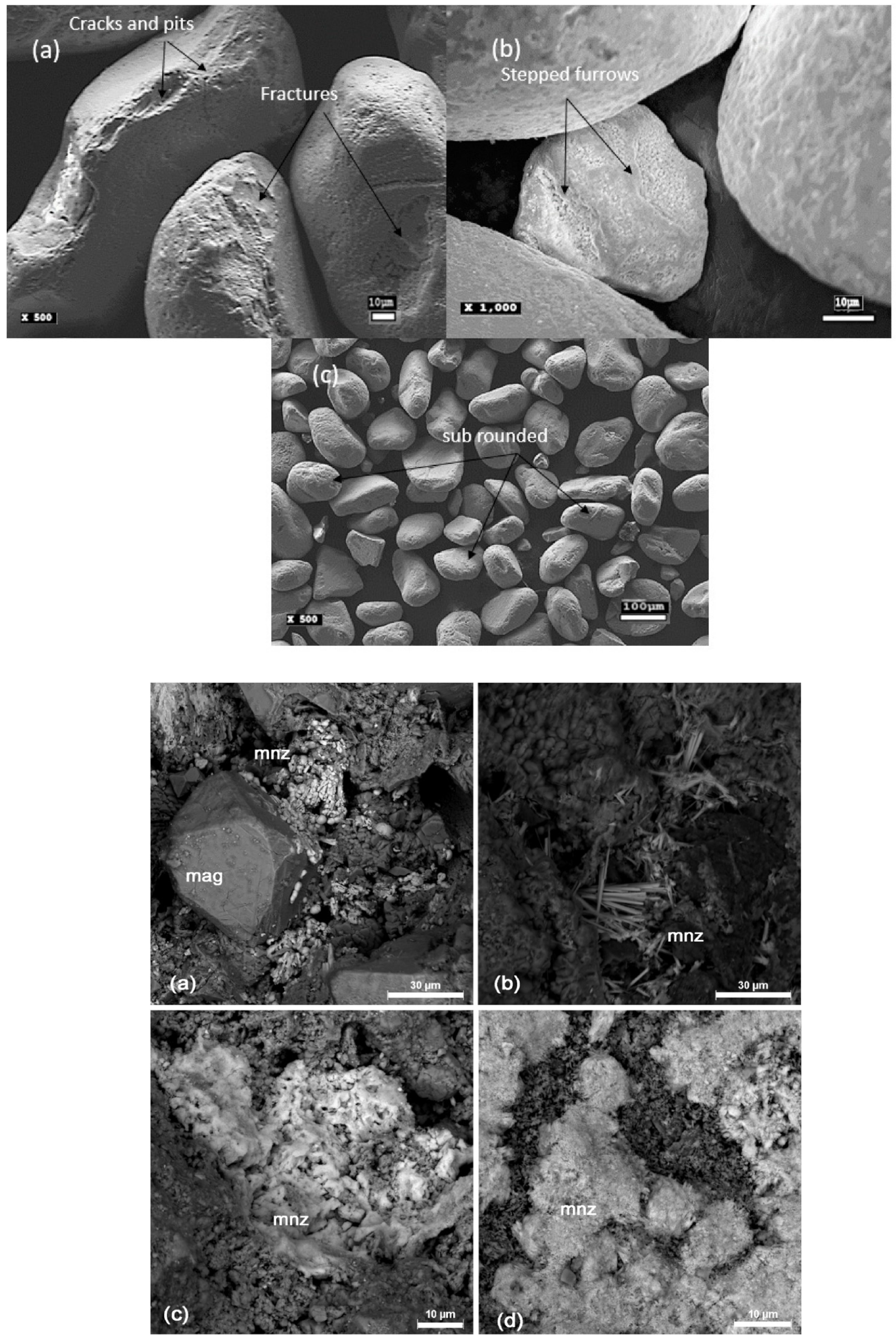
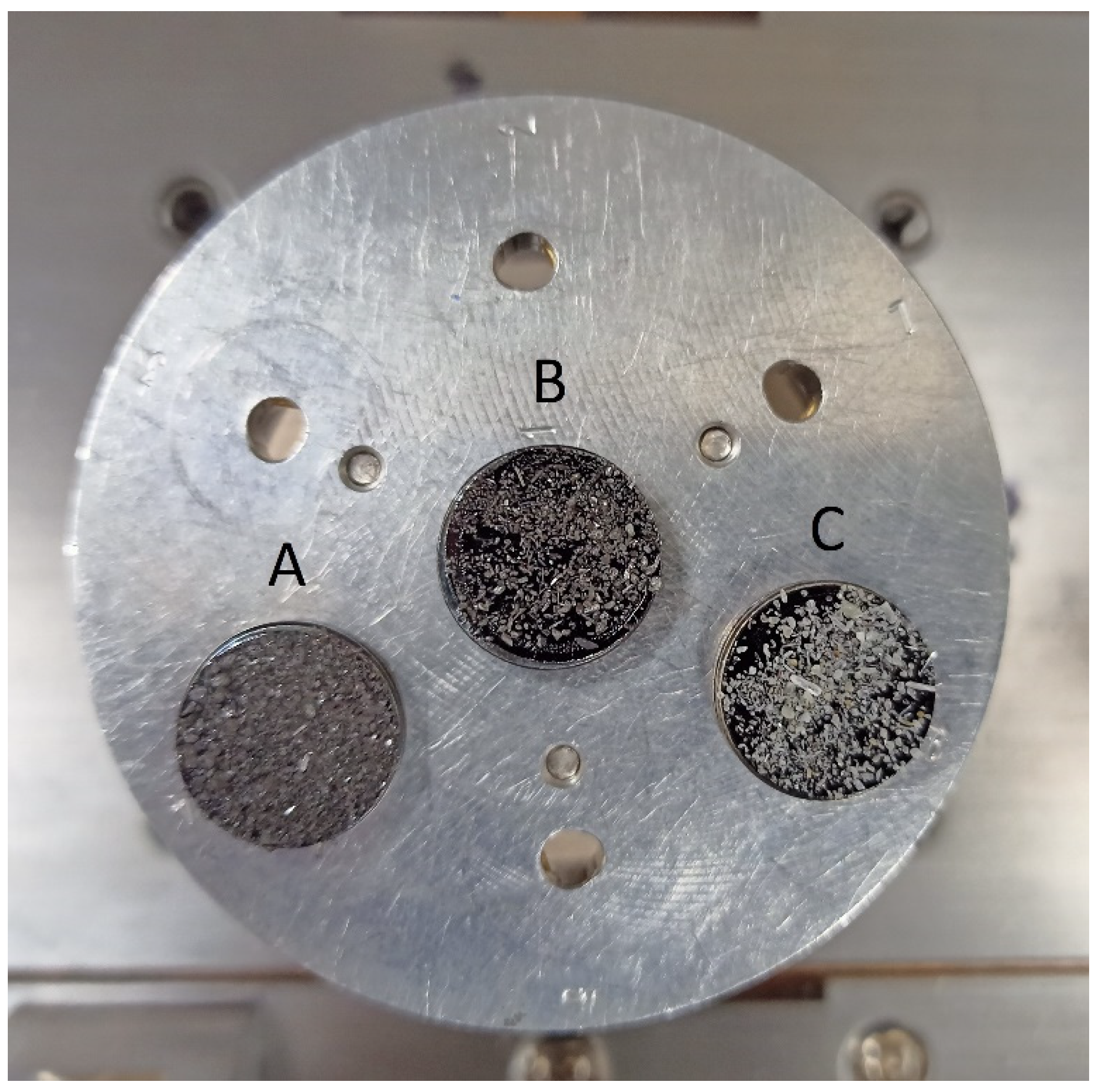
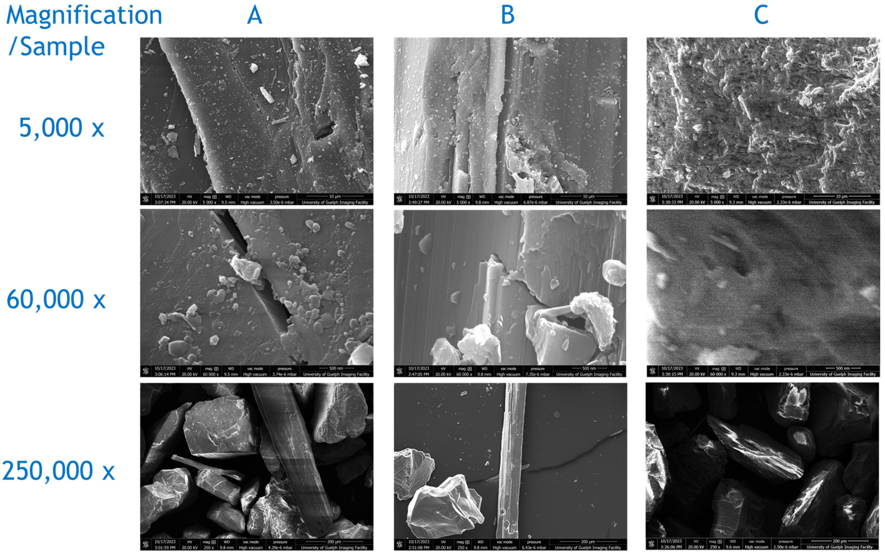
1.2.1. Specimen Preparation

For the production of high-quality and accurate SEM images, the sample preparation stage is very important. SEM analysis is susceptible to distortions, artifacts, and other issues in the case of improper specimen preparation. The sample of interest can be a solid material, a biological specimen, or belong to any other area of the object to be analyzed. The specimen material is mounted on a stub or holder using an adhesive conducting double-sided tape or with other mounting techniques. The SEM stubs are electrically conductive pads. No special specimen preparation is needed for conductor or semiconductor materials. For insulator materials, the image is distorted by charging the sample; therefore, a conduction path to the ground is needed for clear image production [11]. If the sample is moist, the sample must be completely dry before the SEM analysis stage. Moisture can introduce charging effects, thereby distorting the quality of the image. For materials of interest without or with lower electrical conductivity, a thin coating of metal such as gold, platinum, palladium, and chromium is applied to prevent charging effects [51,52,53]. Samples can be trimmed, fractured, or cut to expose the surface of interest to the electron beam and to make the geometry and size of the sample suitable for SEM analysis.

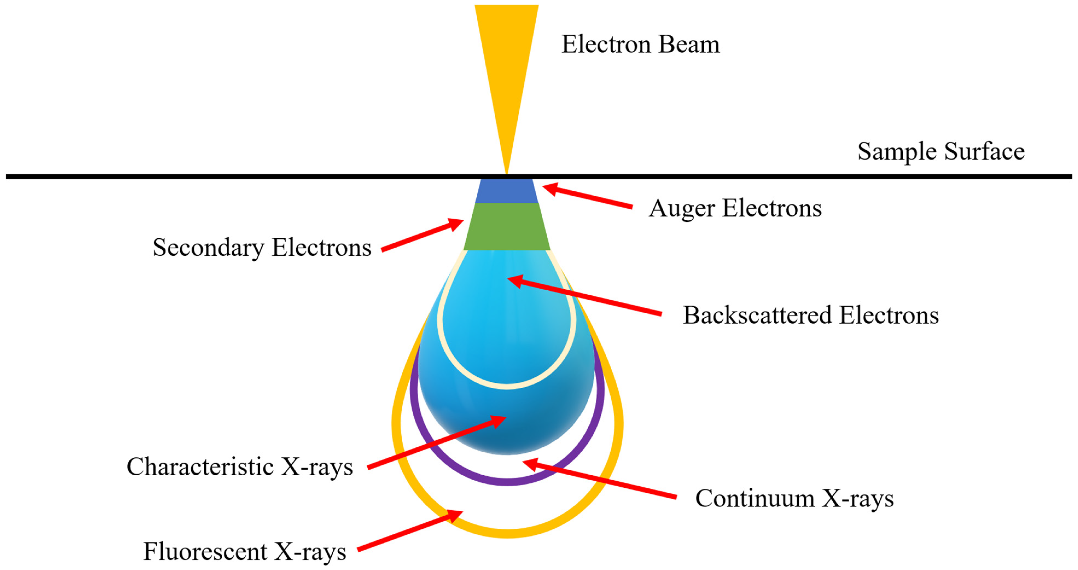
1.2.2. Imaging Process in the SEM

SEM images are formed by using various signals (Figure 2) collected by the detectors present in the collection chamber. Each signal offers different types of imaging information for the sample [11]. Secondary electron imaging (SEI) is an extensively utilized imaging mode in SEM that produces images by detecting secondary electrons [54]. It provides topographic information such as surface texture, shapes, and features. Backscattered electron imaging (BSEI) is generated by detecting backscattered electrons originating from the surface of the sample due to interaction with the primary electron beam [55].

BSE images indicate compositional contrast with respect to the atomic number of the elements present in the sample (Figure 4). This atomic number contrast provides tremendous value in detecting elements in samples containing a variety of chemical compositions. Elements with higher atomic numbers appear brighter in BSE images, while a darker appearance represents an element with a lower atomic number [56,57,58,59]. This feature is especially helpful for mineralogists and geologists because it allows the identification of various mineral phases present in a rock sample. BSE provides value in analyzing the sample surface topography by showing surface texture, morphology, and roughness, which may not be clear in secondary electron images. Certain features of the sample can be studied by BSE contrast enhancement, as it allows the characterization of subtle compositional variations. In Figure 4, the brightness of In_xGa_1−xAs layers (where 0 < x < 0.5) are higher than those of the GaAs layers [57] since the atomic mass of In (114.818 u) is greater than that of Ga (69.723 u). The difference is faint, but still visually noticeable, and the pixelation of the image can be studied by software to assess the locations and widths of the various layers. Monte Carlo simulations and analytical models that consider single electron scattering and electron diffusion can be applied for BSE intensity-based compositional calculations [57]. Notably, the Pt layer on the top portion of the image has the highest brightness given Pt’s large atomic mass (195.084 u). BSE imaging is also helpful in studying nonconductive elements, which is not the case with secondary electron images. BSE imaging can also be coupled with other diffraction and spectroscopy techniques, such as electron backscatter diffraction (EBD) for analyzing the crystallographic properties of materials at a granular level and with energy-dispersive X-ray spectroscopy (EDS) for quantitative mapping of elemental distributions. In Figure 4, this is exemplified by a BSE image of a rock sample that was correlated with EDS of mineral standards to produce the colored image showing in dark blue, blue, light blue, yellow, and red the regions composed of certain mean atomic numbers (Z) [56], including quartz (SiO₂; Z = 10.5; #4); cordierite ((Mg,Fe)₂Al₄Si₅O₁₈; Z = 12.4; #8), almandine garnet (Fe₃Al₂Si₃O₁₂; Z = 13.4; #7), Ti-rich ilmenite (Z = 17.6; #3, #6, #10), Fe-rich ilmenite (Z = 19; #2), and zircon (ZrSiO₄; Z = 23; #1, #5, #9), respectively.

When high-energy electrons coincide with the sample, some materials have the tendency to emit light, and imaging that signal is considered cathodoluminescence imaging (CLI) [60]. The luminescent properties and defects of the sample material are revealed by CLI images. The electrical properties of materials are studied by using the electron beam-induced current (EBIC) technique [61]. It is specifically used for semiconductor materials with localized charge carriers. An electron–hole pair in a semiconductor material is created with the help of the primary electron beam. With the application of an external voltage, the created charge carriers start moving in response to the acting electrical field, indicating a measurable current, which is used to investigate the electrical properties of materials. This technique is also valuable in the identification of defects, grain boundaries, and other microstructural features affecting electrical behavior. The electrical functionality of semiconductor devices is studied with the aid of voltage contrast imaging (VCI), which indicates the variations in electrical potential or voltage across the surface of the specimen [62].

1.3. Fundamental Theoretical Calculations

Crewe et al. demonstrated the basic theoretical calculations in 1969 that were helpful in the design and selection process of SEM [63]. Their work helped in identifying the correct probe size for SEM. The aberrations of the diffraction and electron gun, as well as the first-order image of the field emission tip, aid in determining the size of the examined SEM probe for the specimen. The diameter ($d_s$) of an effective source leads to an image with the following correlation:

$$d_s=2mR{\left(\frac{\overline{v_T}}{v_1}\right)}^{\raisebox{1ex}{$1$}\!\left/ \!\raisebox{-1ex}{$2$}\right.}$$

(1)

where $m$ is the magnification of the gun, R represents the actual radius of the tip, $\overline{v_T}$ indicates the average transverse energy of electrons exiting the tip (~0.2 V), and $v_1$ is the emission voltage needed to produce a 1 µamp emission current. The term ${\left(\frac{\overline{v_T}}{v_1}\right)}^{\raisebox{1ex}{$1$}\!\left/ \!\raisebox{-1ex}{$2$}\right.}$ is the characteristic of a field emission source and indicates the reduction factor of the effective source size.

The theoretical spot size is affected by the aberrations of the gun with the following two terms:

$$d_a=\frac{m{C}_s{\alpha }_1^3}{2}$$

(2)

$$d_c=m{C}_c{\alpha }_1\Delta V$$

(3)

where $d_a$ is the spherical aberration, $d_c$ is the chromatic aberration, $C_s$ is the spherical aberration constant, $C_c$ indicates the chromatic aberration constant, ${\alpha }_1$ is the entrance half angle of the electron beam, and $\Delta V$ represents the total energy spread of electrons. $\Delta V$ is maintained such that the total energy spread of electrons leaving the tip remains at 0.2 V, while variations in $V_0$ and $V_1$ can be considered negligible [63].

At the defining aperture, the diffraction effect should be included. The diffraction contribution to the final spot size ($d_d$) can be calculated as follows:

$$d_d=\frac{0.6m{\lambda }_1}{{\alpha }_1}$$

(4)

where ${\lambda }_1$ represents the electron wavelength at the first anode. The focused spot diameter can be estimated by combining the four terms as follows [63]:

$$d_{rms}=\sqrt{d_s^2+d_a^2+d_c^2+d_d^2}$$

(5)

2. Scanning Electron Microscopy and Mineral Characterization

SEM makes use of secondary electron imaging to analyze the surface topology and morphology of micron/nanometer-scale minerals [64]. For a comprehensive understanding of the microstructure and mineral components, SEM is usually combined with X-ray techniques to complement the acquired information [65,66,67,68]. The infrared spectroscopy method is helpful in identifying chemical species and determining the molecular structure of minerals. This technique has been widely used in mineral characterization [69,70,71,72].

One of the major quantitative analysis methods in mineral analysis is X-ray diffraction (XRD). It correlates the content of minerals with diffraction density, which helps in identifying and quantifying the minerals present in the sample [73,74]. For example, XRD can be used to analyze calcite and nahcolite in saline brine [75], evaluate deposits by identifying minerals in phyllite [76], examine the order degree of dolomite [77], and study the content of calcite and dolomite in carbonate rocks [78]. XRD is a rapid and accurate method for quantitative mineral analysis; however, some mineral compositional structures could lead to errors in analytical results [73].

Combining qualitative analysis with quantification assessment methods can provide a better understanding of the investigated minerals. Such methods include SEM energy-dispersive spectroscopy (SEM–EDS) [78,79,80,81,82], automated SEM mineral liberation analysis (SEM-MLA) [83,84,85], and quantitative evaluation of minerals by scanning electron microscopy (QEMSCAN) [86,87,88]. These methods incorporate a mineral quantitative analysis system by using an energy spectrometer and SEM. For accurate identification of minerals, backscattered electron (BSE) images are used, which can reflect the difference between the X-ray energy spectrum and mineral phase composition [89,90,91]. The quantitative analysis of rare earth minerals is a challenging task with conventional identification methods, and the abovementioned techniques have attained rare earth mineral identification. The problems associated with the usage of these methods pertain to difficulties in application, promotion, and high measurement costs.

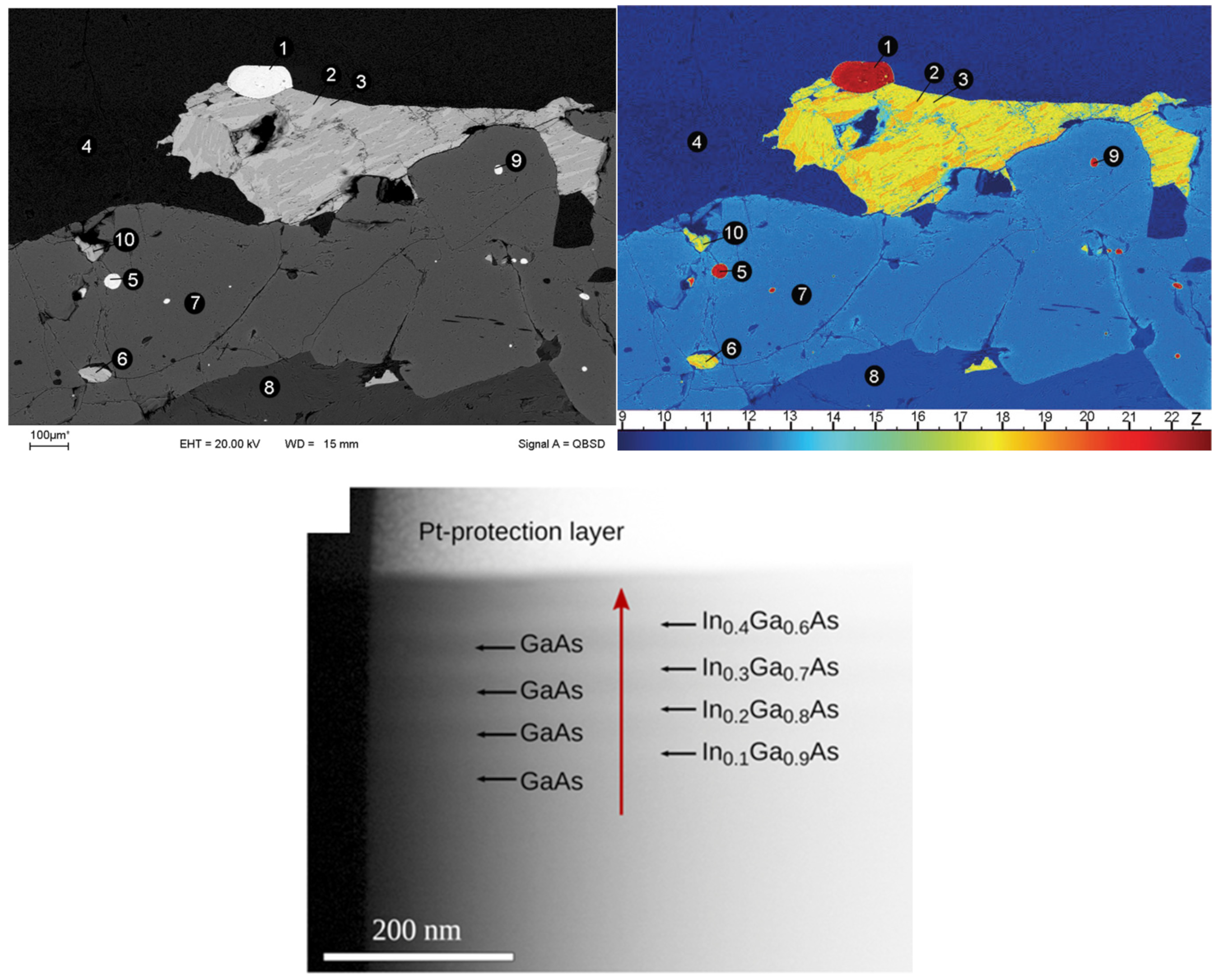
2.1. SEM Energy-Dispersive X-ray Spectroscopy (SEM–EDS)

When the electron beam emitted from the gun penetrates and interacts with the volume beneath the sample surface, X-rays are generated. This is a well-established principle in physics: the deceleration of electrons due to their entrance into the Coulomb field of the specimen results in a loss of electron energy and emits photons. In SEM analysis, similar X-ray photons are emitted, which are characteristic of the sample under investigation [89], as shown in Figure 2.

The quantification scheme is achieved by measuring the X-ray intensity. This was illustrated by Heinrich and Yakowitz in 1968 in their publication, Quantitative Electron Probe Microanalysis [92], which later became the standard for developing X-ray fields. At that time, X-ray absorption, determination of correction factors at the instant of electron penetration and scattering, and conversion of X-ray intensity to the relative concentration were missing. Many problems pertaining to the electron probe field were solved with the development of energy-dispersive spectrometry (EDS). At present, various studies have incorporated SEM–EDS for qualitative and semiquantitative analysis in a variety of subject areas [93,94,95,96,97,98,99].

A schematic diagram of an energy-dispersive spectrometer is shown in Figure 5. The X-ray detection system (which is a solid-state detector) separates the characteristic X-rays of various elements present in the sample. Then, the EDS system software analyzes the energy spectrum to determine the amplitudes of particular elements, and electrical signals are generated from the respective photon energies. This results in qualitative and quantitative determination of a chemical composition map of the elements present in the sample [89]. SEM–EDS has been used in a variety of fields for mineral characterization [100,101,102,103,104,105,106].

2.2. SEM-Based Automated Mineralogy (SEM-AM)

SEM-AM is a tool that was initially designed to characterize mineral processing products and ores. The measurement process starts with collecting backscattered electron (BSE) images, which are analyzed using image analysis software procedures. Based on BSE image adjustments, the energy-dispersive X-ray spectra (EDS) are obtained at selected points. The EDS spectra of the sample are then classified based on the list of approved reference EDS spectra. Relevant software providers offer services such as particle analysis, EDS spectral mapping, sparse phase search, and point counting modal analysis using four principal SEM-AM measurement routines and different classification algorithms, which can be used based on the analysis requirements. The main challenges associated with the process are materials with very different hardnesses, polishing relief surfaces of particles, electron beam stability, and appropriate nonevaporating epoxy resin mixtures [84].

SEM-based automated mineralogy (SEM-AM) is still underutilized, although SEM instruments are widely distributed in industry, geosciences, and materials research. SEM-AM can produce valuable results for a variety of major applications by characterizing the primary ores and optimizing mineral concentration, flotation, comminution, and metallurgical processes in the mining industry through the generation of quantified reliable data [107,108,109,110,111]. Beyond the classical fields, the potential of SEM-AM has gained further interest on scientific and economic grounds. Some closely related topics are ore fingerprinting, metallurgy, and applications in petrology [112,113,114].

SEM-AM systems are a combination of hardware platforms, processing software, and specific image analysis. Any SEM with minor adjustments can be used as a hardware tool for SEM-AM. These adjustments include a high vacuum operation mode and additional internal mainboards. A vacuum pressure of 10⁻⁵ to 10⁻⁷ Pa is needed for its operation. Electron sources of tungsten cathodes and field emission guns can be employed. Tungsten cathodes can be used for economical operation; however, field emission guns are recommended for the long-term stability of electron beams for automated measurements. The speed of analysis and X-ray count rate are increased in SEM-AM by employing two or more EDS spectrometers in the SEM hardware. Multiple samples can be accommodated in a large sample chamber for simultaneous analysis in a single measurement session. A very accurate stage movement of SEM allows precise positioning using small intervals. For valuable analysis results, a fine-quality backscattered electron (BSE) detector is needed. In SEM-AM analysis, BSE image quality and stability are important factors, as the resultant image (in combination with the EDS spectrum) is used for phase or mineral discrimination. Prior to measurement, fixed working distances must be set to keep the BSE image gray levels constant [84].

Keeping the image calibration constant ensures that a specific phase or mineral always possesses the same BSE image gray level. The calibration process can be conducted with various BSE image gray levels of reference materials such as quartz (dark gray), copper (intermediate), and gold (very bright) [84]. The choice of calibration reference material should be made based on the sample material to be investigated. For example, many slags, industrial ash, or particulate materials are investigated using SEM-AM, and quartz or copper are used for calibration with dark gray to intermediate BSE image gray levels. This results in SEM images with better resolution and quality. For SEM-AM technology, four principal measurement routines can be outlined, which starts with collecting BSE gray-level images with respect to the calibrated gray level, as shown in Figure 6. The upper row represents the BSE images, while the bottom row indicates the EDS images of SEM-AM of one measurement frame. White or black crosses denote the points of X-ray analyses (only some points are shown). Figure 6 presents the EDS point counting technique used for the quantification of modal composition. Figure 6 shows particle analysis by EDS, which has been developed for fast automated characterization of grain mounts with up to 10⁶ particles, such as milled products from mineral processing and mining. Figure 6 illustrates the sparse phase search method, which combines single spot EDS spectral analysis of grains with a BSE gray tone value trigger. It is valuable in massive rock applications, such as drill cores and thin sections. Figure 6 demonstrates EDS spectral mapping, which combines BSE image levels with mapping of the EDS spectrum. This method is helpful, especially in cases where fine details of mineral intergrowth are considered. In summary, SEM-AM is a powerful tool for mineral characterization and has actively been used in recent literature [115,116,117,118].

2.3. Automated SEM Mineral Liberation Analysis (SEM-MLA)

Recent software developments in SEM have incited dominant growth in its application in solid matter investigations. One of the economic solutions is the use of mineral liberation analysis (MLA) for optimizing the mineral processing methodology of metallic ores. SEM-MLA has been an important driver in transforming numerous software versions for SEM applications [84]. SEM-MLA was designed to quantify the mineralogy of ores. After the mining process, the ore is processed to increase the concentration of minerals of interest (and value). The processing of ores is also important for removing minerals of no value or those with detrimental effects on the needed mineral products. This processing of grinding the ores and liberating the minerals of interest provided rapid automated analysis of target minerals and extensively improved the process.

A mineral liberation analyzer (MLA) based on SEM was developed in the late 1990s by the JKRMC (Julius Kruttschnitt Mineral Research Centre, Australia), and it is currently commercially available [118]. In MLA, minerals are differentiated by attaining and combining the information gathered from EDS and BSE. Depending on the size range of the particles in the sample, size fractions from the sample are produced. Then, liberation is measured in each size fraction, followed by liberation reconstruction of the whole sample. The measurement of mineral liberation is usually carried out through one of two methods, i.e., either the area method or the linear intercept method. Liberation by area measurement has shown lower stereological error compared to linear measurement.

It is important to note that liberation measurements by the linear intercept method are known as one-dimensional, while area method measurements are called two-dimensional liberations. Both of the measured liberations are lower dimensional projections of the true volumetric liberation, which is three-dimensional. Stereological correction is based on stereological transformation and prediction of liberation measurements. This stereological correction can be based on entropy regularization [119]. Correction of the apparent liberation and production of three-dimensional liberations have also been described in several other investigations [120,121,122]. Various operating modes for the MLA system are available, i.e., X-ray modal analysis (XMOD), particle X-ray mapping (PXMAP), selected particle X-ray mapping (SXMAP), sparse phase liberation analysis (SPL), standard BSE liberation analysis (BSE), extended BSE liberation analysis (XBSE), and rare phase search (RPS) [123]. The use of SEM-MLA is shown in Figure 7 for quantifying the mineralogy of a hydrothermally overprinted alkali plutonite [85].

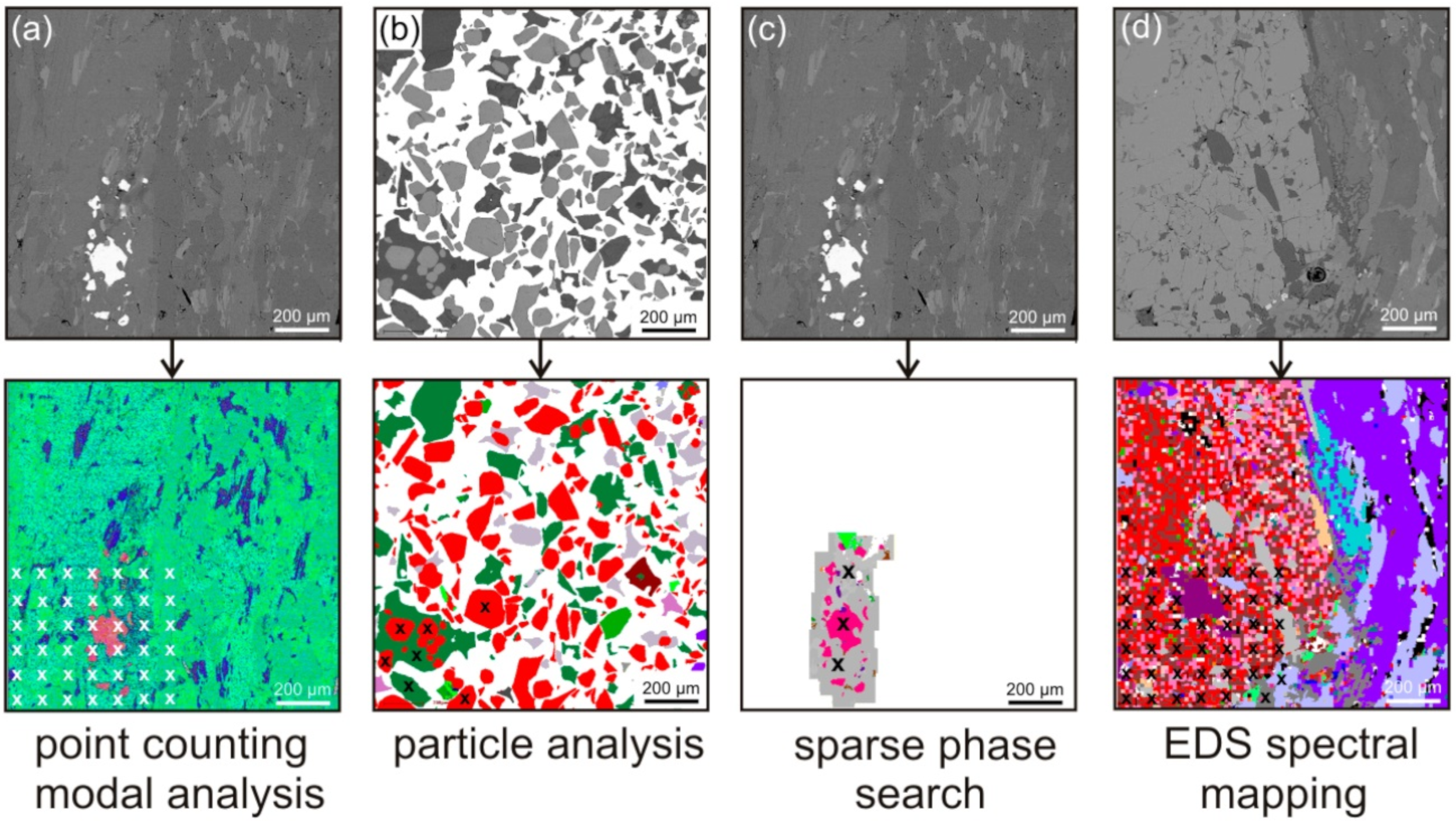
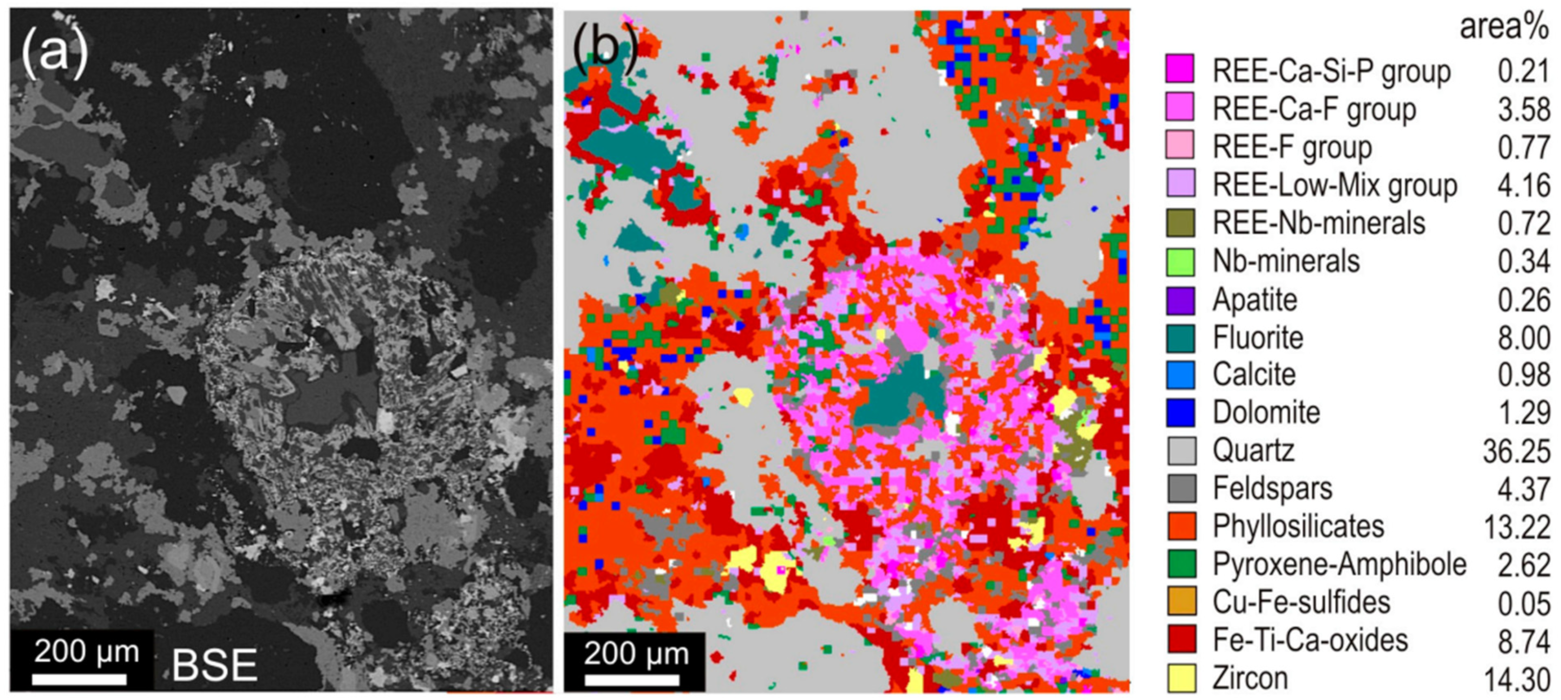
2.4. Quantitative Evaluation of Minerals by Scanning Electron Microscopy (QEMSCAN)

Traditional mineral analysis based on microscopy cannot provide the needed data because of the absence of quantitative information and the very small size of the particles of interest. QEMSCAN technology, initially termed QEM*SEM, demonstrated the potential to revolutionize automated mineralogy [124]. In a mold, the particulate mineral sample is mixed with epoxy resin, and the sample surface is prepared using cutting, polishing, and carbon coating. The sample is scanned using SEM in backscatter mode, enabling the differentiation of particles from the background. After the identification of particles on the resin block, their composition is systematically mapped using EDS. In contrast to the most modern SEMs coupled with single EDX, QEMSCAN possesses the attribute of having multiple EDXs at the same time, enabling rapid quantitative mineralogy. The acquired EDX signals are then compared with reference known materials in the database and assigned a mineral name or to a chemical compositional grouping. With this process, the mineralogy of the sample can be determined by particle-by-particle analysis [124]. QEMSCAN locates the particles using a BSE signal, while identifying the mineral by an EDS signal. It can be compared to SEM-MLA, which makes more use of the BSE signal than EDS for identifying the mineral. SEM-MLA works very well for bright phases (such as platinum group element minerals).

Among SEM–EDS techniques, QEMSCAN is one of the most widely used and offers quantitative characterization of minerals, ores, and other mineralogical compounds [125,126,127,128,129]. QEMSCAN is usually used in conjunction with other analytical techniques, such as electron probe microanalysis (EPMA) and X-ray diffraction (XRD), as shown in

Table 1. Techniques used for investigating mineralogy and their comparison. ✔ indicates good, ● represents poor, while ▲ suggests it is possible but not recommended [130].

Investigation	Electron Microprobe	XRD	QEMSCAN
Mineral texture	▲	●	✔✔✔
Mineral distribution and associations	▲	●	✔✔
Mineral-specific particle size information	▲	●	✔✔
Mineral abundance	●	✔✔✔	✔✔✔
Amorphous minerals (geothite, silica)	✔✔✔	●	✔✔✔
Distribution of minor metals within minerals	✔✔✔	●	✔
Crystallinity (clay, silica, geothite, and limonite)	●	✔✔✔	●

[130]. Figure 8 indicates the use of QEMSCAN for identifying the mineral distribution of four samples [130]. It shows the presence of geothite, quartz, clay, limonite, and other silicate minerals.

The above-described four analytical techniques are distinct but complement each other in comprehensive mineralogical analysis. High-resolution images are provided by SEM, elemental composition analysis is provided by EDS, and SEM with automated mineralogy involves a thorough mineral characterization. Most SEMs with automated mineralogy equipment incorporate EDS, where software utilization provides objective and quick mineral characterization and other analytical results. QEMSCAN is a specific instance of the broader concept of automated mineralogy, which represents a specific system and brand used for comprehensive mineral characterization. MLA systems are used in geology, mining, and mineral analyses for ore processing and beneficiation, as they provide insight into the degree of liberation of valuable minerals from the host rock. Combining these techniques offers constructive value to mineral characterization and the analysis process by not only providing high-resolution surface images but also offering the elemental composition of the sample, the degree of liberation of minerals, and saving time in determining the presence of valuable minerals present in ores. In short, SEM is a powerful technique for the characterization and analysis of various minerals [131,132,133].

Mineral characterization is usually carried out with more than one technique for clear identification and quantification. Therefore, SEM analysis for mineral characterization is accompanied by several other analytical techniques, as mentioned in

Table 2. Recent SEM applications focusing on mineral identification, quantification, and characterization.

Analytical Methods/Techniques	Year	Minerals/Materials	References
SEM/SDD-EDS, EPMA-WDS,	2023	Major and minor elements in minerals and rocks	[134]
SEM–EDS, XRD	2022	Constituent minerals in shales	[135]
SEM, TEM	2018	Microbial biofilms, mineral precipitation	[136]
SEM-BSE, TMR, SMH	2018	Mineral content in enamel lesions	[137]
SEM, µXRF, LWIR, SAM	2020	Quartz, olivine, kyanite, and diopside	[138]
SEM–EDS, Raman Spectroscopy	2019	Asbestos	[139]
SEM-EDX, XPS, XRD, FT-IR, UV	2020	Kaolin, illite, gibbsite, and quartz	[140]
SEM, XRD, TGA, IR, TXRF	2022	Mineral constituents in human renal calculi	[141]
SEM-FIB	2021	Mineralized bone	[142]
SEM–EDS	2021	Mineralizing fluids, sedimentary brines	[143]
SEM-FIB, µCT, XLH	2020	Crossfibrillar mineral tessellation	[144]
SEM, BSE, EDS,	2022	Sandstone	[145]
SEM, CT, Raman Spectroscopy	2021	Saturated brine, wellbore cement	[146]
SEM–EDS, XRD, IRS, XRF	2023	Gabbro-anorthosite, seawater, and mafic rock	[147]
SEM–EDS, AM-SEM, FE-SEM, CT	2023	Mineralogical analysis of petroleum geology	[148]
SEM-FIB	2020	Mineralized scale patterns on the cell periphery	[149]
SEM, EMP, Raman Spectroscopy, BSE	2019	Petrified wood, Mn-oxide minerals	[150]
SEM–EDS, Monte Carlo Simulations	2021	Glass fiber-reinforced cement	[151]
SEM, XRD, XRF, FTIR	2022	High ash coal, fluidized bed gasifier	[152]
SEM–EDS, XRD	2023	Mineral-forming bacteria	[153]
SEM–EDS, XRD, TGA	2023	Self-healing cement-based minerals	[154]
SEM, XRD, XPS, FTIR	2023	Biomimetic mineralized cement	[155]
SEM, TEM, PLM, EBSD, SAED	2023	Talc, amphiboles, and biopyriboles	[156]

SEM = Scanning Electron Microscopy, SDD = Silicon Drift Detector, EDS = Energy-Dispersive X-ray Spectroscopy, EPMA = Electron Probe X-ray Microanalyzer, WDS = Wavelength-Dispersive Method, XRD = X-ray Diffraction, TEM = Transmission Electron Microscopy, BSE = Backscattered Emission, TMR = Transverse Micro-Radiography, SMH = Surface Micro-Hardness, µXRF = Micro X-ray Fluorescence, LWIR = Long Wave Infrared, SAM = Spectral Angle Mapper, EDX = Energy-Dispersive X-ray Spectroscopy, XPS = X-ray Photoelectron Spectroscopy, FT-IR = Fourier-Transform-Infrared Spectroscopy, UV = Ultraviolet Visible, TGA = Thermogravimetric Analysis, TXRF = Total Reflection X-ray Fluorescence, FIB = Focus In Beam, µCT = X-ray Micro-Computed Tomography, XLH = X-Lined Hypophosphatemia, IRS = Infrared Spectrometry, AM = Automated Mineralogy, FE = Field Emission, EMP = Electron Microprobe, PLM = Polarized Light Microscopy, EBSD = Electron Backscatter Diffraction, SAED = Selected Area Electron Diffraction.

, which have been applied in some recent publications.

3. Uncertainties, Limitations, and Sources of Error in SEM Measurements

The advancement of SEM with automated mineralogy has provided a quick and relatively economical quantitative mineral analysis solution. However, the absence of statistical errors makes the robustness of the results uncertain. This could damage the reliability of technical solutions taken on the onus of these quantitative outcomes [157]. Automated mineralogy-based measurements have been studied with several methods for the estimation of uncertainties. For instance, a statistical approach was developed by Benvie et al. in 2013 for using SEM automated mineralogy in accordance with diagnostic leaching tests [158]. It was concluded that to derive the standard deviation and background variance, at least two grain mount measurements were needed for each head and leach residue sample. In another study, the variability in mineral liberation analyses and mineral quantity was investigated by Lastra and Paktunc in 2016 [159]. They studied the fraction of sulfide flotation rougher concentrate of −509 to 208 µm in size through interlaboratory testing. Mineral quantities were found to have good agreement with the data, but mineral association and liberation analyses showed less agreement. This finding hints toward the idea that correct mineral liberation and association may not necessarily be found with correct mineral quantities. In 2021, Guseva et al. evaluated the analytical errors in mineralogical measurements by applying the point counting method via binomial distribution approximation [160]. Binomial approximation may not fit well with all cases, especially with coarse materials, and suitable methods for each case should be used, such as estimation of the confidence method [161] or the bootstrap resampling method [162].

The estimation of errors in textural characteristics measured by automated mineralogy can be efficiently identified using the bootstrap resampling method [163]. For instance, the bootstrap approach can help in evaluating the uncertainties related to particle properties measured by SEM automated mineralogy for the evaluation of magnetic separation efficiency [164,165], density separation processes [166], and the simulation and statistical modeling of mechanical separation processes [167]. The bootstrap resampling method considers a population of N samples, takes M random subsets, and replaces the randomly selected samples to ensure that the entire population is available for sampling [168,169]. The accepted statistical methods, which use the point counting method on polished sections and assess errors in mineral grades, agree well with the bootstrap method [170,171,172]. This method has the advantage of being assumption-free and can be applied to a wide range of particle characteristics [162]. It does not assume a bionomical distribution. These methods imply that the standard deviation of mineral grades is proportional to the square root of the number of particles measured or the total area of particles measured. The relative standard deviation of measurements for any mineral grade can be estimated as follows [173]:

$$RSD=a{x}^{-0.5}$$

(6)

where $RSD$ is the relative standard deviation, $a$ is a coefficient, and $x$ is the mineral grade.

The bootstrap method can also provide information about the measurement of how much total area (grains) is needed to reach a given uncertainty. In addition to the uncertainty, SEM also has some drawbacks, including (but not limited to) limited depth of penetration that primarily provides surface information; and low accelerating voltages that provide low-resolution images, while increasing the voltage starts damaging the surface of the sample.

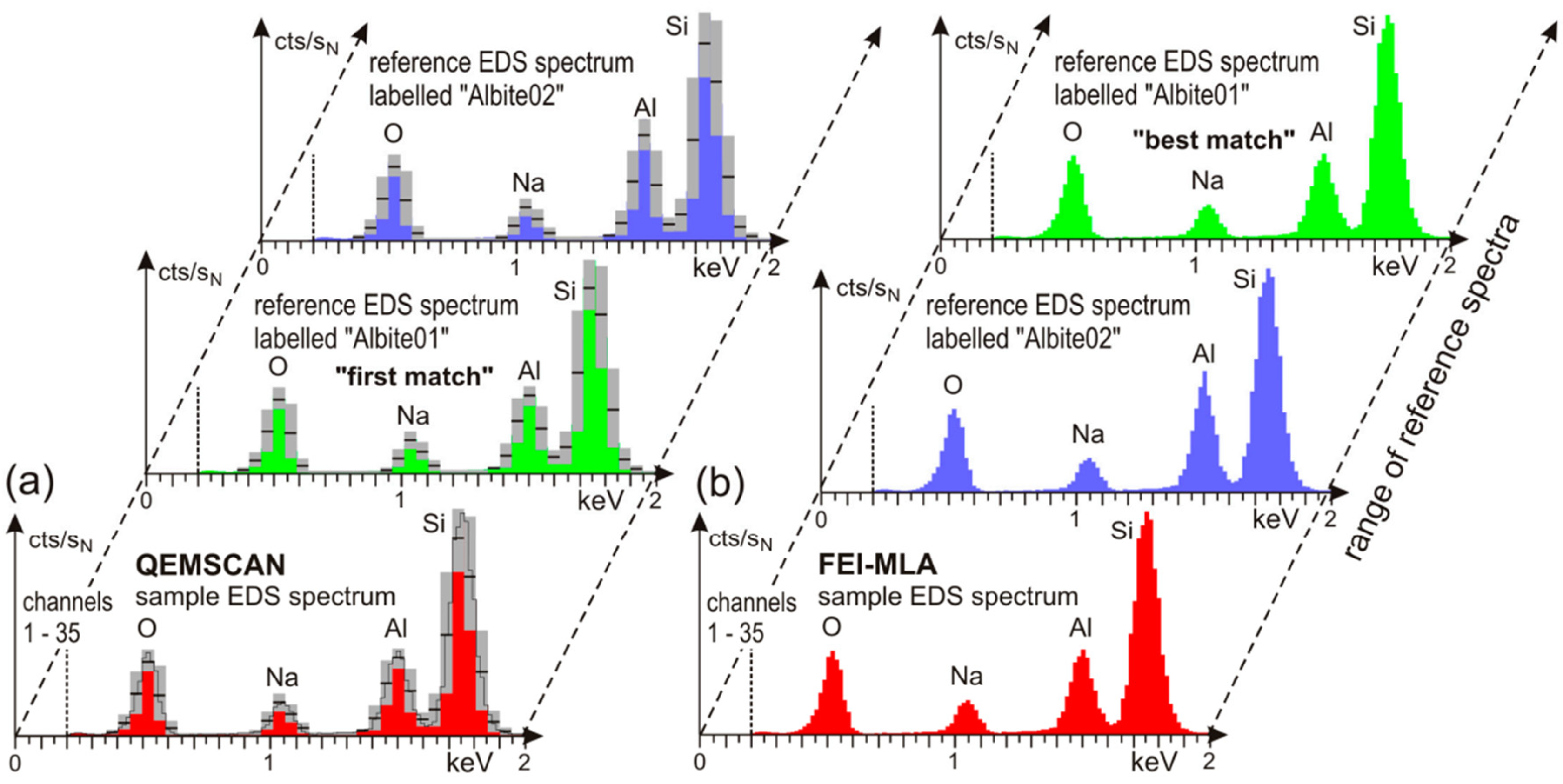
3.1. Constraints in Phase Identification by EDS Spectra

It is a common claim in SEM-based automated mineralogy studies that minerals can be detected, identified, and quantified by their characteristic EDS spectrum (an example is shown in Figure 9, indicating feldspar mineral albite [84]). However, this claim cannot be fully correct, as minerals are characterized by their lattice structure indicated by XRD first, and then comes the use of elemental composition information provided by EDS spectrum quantification. Therefore, mineral identification remains incomplete with use of the EDS spectrum only, based on its foundations on elemental composition. Identifying a mineral by chemical composition alone can be misdirecting, as there are examples of minerals with similar chemical compositions but different crystal structures based on the crystallization conditions of minerals. For instance, pseudorutile and ilmenite are both titanium-iron oxide minerals, but they exhibit different crystal structures [84].

Another challenge in mineral detection, identification, and distinction using EDS spectra is that some minerals have very similar elemental compositions, such as hematite (Fe₂O₃) and magnetite (Fe₃O₄). Hematite is composed of 70% by weight Fe and 30% by weight O, while magnetite is made up of 72% by weight Fe and 28% by weight O. The EDS spectra for both minerals appear to be very similar, and the very trivial differences in Fe and O peaks cannot be resolved by appearance. In such scenarios, it is a good idea to use the BSE image gray level as an additional distinguishing standard. It must be noted that for such a measurement, a specific BSE brightness and contrast calibration is needed. Another challenge is the detection range of EDS spectra, as it does not cover the whole elemental periodic system. For example, the first light elements cannot be detected by EDS, such as H, He, Li, and Be. It is, therefore, recommended to complement EDS spectra with XRD and XRF methodologies for mineral identification and quantification [84]. Other limitations of EDS spectra include longer mapping causing damage to the samples, low sensitivity of light elements, low quantitative accuracy, information about the chemical composition only (not about functional groups or chemical bonds), and overlapping peaks, making it difficult to distinguish among elements present in the sample.

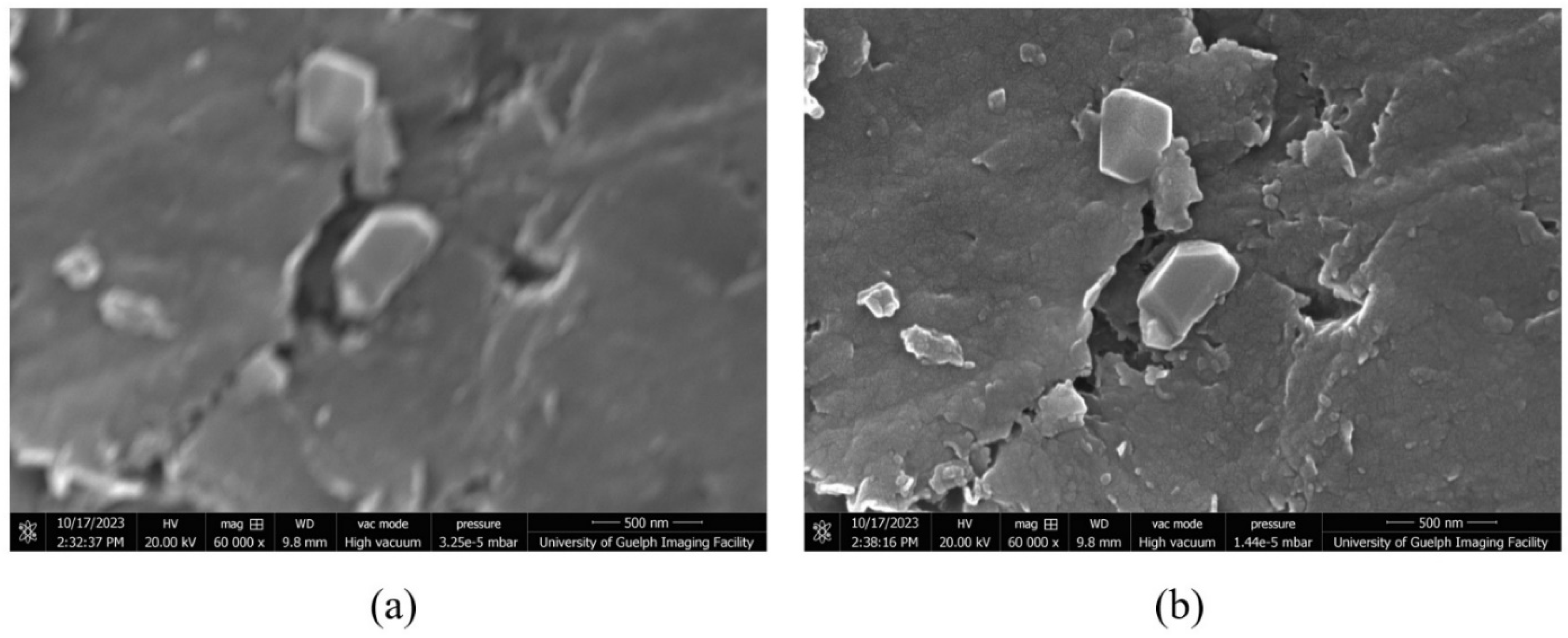
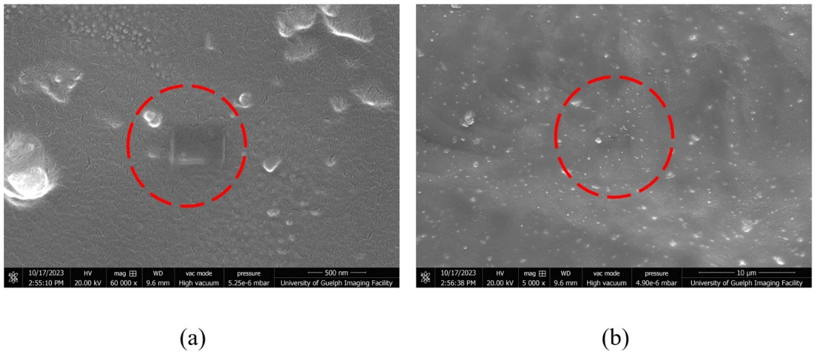
3.2. Sample Preparation and Related Issues

For the success of any SEM analysis, an optimal sample preparation process is essential. A wide variety of samples can be analyzed using SEM. The configuration of the sample holder system and the size of the SEM sample chamber are the defining parameters for choosing the type of sample for investigation. Grain mounts in round epoxy blocks are usually used for particulate or granular samples. If the samples are massive and contain compact matter, such as rocks, petrographic glass-mounted sections can be used. Depending on the type of sample, the production of thin grain mounts on glass is also possible. Two important configurations must be maintained, whether they are samples on glass or round block sample holders, i.e., the holder should be mounted perpendicular to the electron beam and parallel to the BSE detector [84].

Grain mounts in epoxy blocks are the best form to prepare samples if the sample material is noncompact, particulate, or granular, which can be ground, hand-picked single, or broken grains [174]. A potential problem occurs when the grains are not easily separated within the same colored grayscale BSE image, as most SEM-AM software packages are unable to distinguish between them. The use of pure graphite is beneficial in such cases, as it can be utilized in stirred form as a distance material into epoxy resin blocks [174]. In some granular sample cases, a wide range of densities can exist among the phases present in the sample. During the stirring process of sample grains with graphite-saturated epoxy resins, grains with larger sizes and high densities tend to move toward the bottom of the holding block, and it is more probable that small grains will be missed in the analysis. One good practice for dealing with such kinds of samples is cutting round blocks into vertical slices, which can be remounted as vertical sections [84]. It is also possible to study other materials, such as polymers and coal, with the use of EDS detectors. Since the BDE gray value of this organic matter is similar to that of epoxy resin, an alternative embedding material should be used [175]. Carnauba wax is an alternative material that can be used for embedding in these cases [176]. Carnauba wax is a very soft material, making it difficult to polish. One possible solution is to double-mount the Carnauba wax in epoxy resin blocks. Another prospective solution could be the doping of iodoform in epoxy resin [175,177]. The organic matter has a lower atomic number than the epoxy resin, which makes the epoxy a background material. A wide variety of epoxy resins are available for this purpose [178]. SEM images of some epoxy resins and their respective thermal conductivities are shown in Figure 10. In addition to the variety, the proportions of hardener and filler can be varied. The challenges in choosing an epoxy resin are that it must remain stable under a 25 kV electron beam, not evaporate under high vacuum conditions, and harden within convenient temperature conditions and time frames. The recommended approach to solving such problems is continuous application tests.

The complications associated with the sample preparation procedure depend on the type of sample material. If it is solid, dry, compact, and massive, the preparation of thin and thick sections is quite simple. In the case of brittle and/or porous material, epoxy resin is impregnated with a previous material for stabilization before sawing. Thin and thick section production has been reported by several studies [180,181,182]. Usually, silicon carbide (SiC) with 600 to 1000 mesh is used for lapping of the sample material behind the mounting on glass. In the standard lapping procedure, SiC 1000 works best for brittle and soft materials, with minimum substance loss compared to SiC 600. If the sample contains minerals with different optical properties but a closer chemical composition, thin sections are advantageous as an optical microscope can also be used to check the minerals and phases. In addition, a microscope with polarized light can be used to recognize samples with glassy phases owing to their optical isotropy. The reference EDS spectra list can be compiled based on this set of information [84].

A plane and well-polished surface is needed for SEM-AM to analyze grain mounts of thin and thick sections and mounts in epoxy resins. Every material needs a specific treatment, so it is safe to state that the polishing part is a work of craftsmanship. In most cases, water is used in the polishing procedure. If there is a chance of water reacting or mixing with the minerals or materials, the sample preparation procedure can be carried out with water-free liquids such as ethylene glycol [84]. A variety of industrial ashes, such as power plant and sewage ashes, can contain anhydrite, and the use of water-free liquids is recommended in such cases. For samples with varying degrees of particle hardness, covering the polishing plates with hard textile cloth is proposed. Plates covered with soft cloth having long fibers work well for samples containing minerals, soft metals, or ore minerals. The procedure of polishing the sample works well with decreasing grain size, for example, using abrasive papers first, then grinding, and then polishing powders on textile cloth. It is important to mention avoiding the use of lead-bearing polishing plates for general sample preparation, as it may cause sample contamination with lead. For the last step of sample polishing, the use of diamond powder with diamond paste or lubricant is very effective. The polishing procedure can be controlled using a reflected light microscope to inspect the level of successive polishing steps. The impinging electrons in SEM should be dissipated well to obtain optimal BSE images. The use of carbon coating on polished samples provides a solution, which can be accomplished by either evaporation of carbon-loaded thread, electronic carbon thickness control, carbon rods, etc. [84].

The quality of SEM images in publications is essential for clear communication and interpretation. It is also significant for ensuring reproducibility and avoiding hindrance in future research directions. Blurry SEM images also cause limitations in quantitative data extraction and challenges to peer reviewers in analyzing, interpreting, and understanding the results. Low-resolution images in scientific papers appear for several reasons, some of which may be unintentional, while others are the result of constraints or limitations of the research process. The common reasons for the presence of low-quality SEM images in papers may include (but are not limited to) instrument limitations, sample conditions, resource constraints including time and budget, image processing and acquisition, sample size, scope of the paper, image compression, historical or legacy data, data storage, and file size. To produce focused and clear SEM images for the efficient transfer of information, the stigmator tool in the SEM instrument should be properly utilized.

The stigmator is one of the critical components of the SEM instrument and is responsible for maintaining the astigmatism of the electron beam and adjusting the focus of the SEM equipment. While examining the fine details of mineral structures, astigmatism can cause distorted and blurry images. The stigmator ensures the symmetry and focus of the electron beam, consequently producing quality SEM images. The proper use of a well-adjusted stigmator allows characteristic mineral identification, enhanced elemental analysis, quantitative analysis, and precise imaging of microstructures. It also helps in enhancing images of thin sections and provides crystal clear information about crystal faces, surface roughness, and other textural attributes, which is essential for understanding the formation of minerals and digging deep into the geological history of minerals.

Figure 11 shows wollastonite samples mounted on three stubs, as described in

Table 3. Wollastonite samples prepared for SEM analysis.

Sample	Layer	Sputter Coating
A	Multiple	Applied
B	Single	Applied
C	Single	Not Applied

. Figure 12 shows the effects of layers and sputter coating on SEM analysis by comparing wollastonite samples A, B, and C for three magnifications, i.e., 5k×, 60k×, and 250k×. In the sample preparation stage, sample C was left uncoated to investigate the effect of sputter coating, while samples A and B were coated with gold-platinum coating. It is clearly illustrated in Figure 12 that all SEM images of sample C are fuzzy and dark with few very bright spots and lines, making it difficult to visualize the sample morphology. This is the charging effect, logically occurring due to the absence of a conductive material coating. Another important aspect can be found by comparing the 60k× and 250k× SEM images of sample C with its 5k× image. While charging effects are prominent in all SEM images, that with lower resolution provides better visualization of features when compared to the ones at higher resolution. This suggests that for samples that are difficult to coat with conductive materials, it is useful to capture SEM images at lower resolution. When comparing the SEM images of samples A and B, it is observed that the morphology of the sample can be well studied with single-layered samples compared with multilayered samples.

To ensure that the stigmator is well adjusted for taking quality SEM images, the SEM instrument should be allowed to stabilize and warm up, which will ensure that the electron source and other components of the instrument are at steady state before any adjustment. There are usually two stigmation modes in SEM, i.e., objective lens stigmation and condenser stigmation. The specific requirement of the imaging task will require the selection of an appropriate stigmation mode. Misalignment in electron columns and detectors can adversely affect SEM image quality, which is why it is important to ensure proper alignment of these components before starting the imaging process. Some of the latest SEMs include automated alignment features. The sample preparation stage is also important for avoiding any contamination and charging effects hindering image quality. Dry, clean, and well-mounted samples provide a foundation for high-resolution SEM imaging. While focusing the electron beam on the sample, it is necessary to adjust the astigmatism controls to obtain a sharp image at low magnification. It is considered good practice to select a well-defined edge or feature on the investigated sample as a reference point for stigmation control adjustments. Astigmatism is usually indicated by distortions in the SEM image, such as asymmetrical or elliptical features. In the SEM imaging process, it is important to observe such biases. The X- and Y-stigmation (representing horizontal and vertical stigmation, respectively) need to be adjusted to eliminate any distortions. The focus of the electron beam should be rechecked and adjusted, if necessary, for proper and clear imaging. For optimal SEM imaging, several iterative adjustments might be needed. Figure 13 compares the stigmator adjustment effect on SEM images, which vividly indicates the importance of stigmator adjustment in SEM analysis. Additionally, Figure 14 shows the effect of maintaining the electron beam for a longer period of time at a single point, which damages the surface of the sample (rectangle marks indicated by dashed circles). This issue can be resolved by reducing the voltage of the electron beam, but that comes at the expense of lower resolution of the SEM image. Therefore, it is recommended to find an optimum voltage–resolution combination that works well for a specific type of sample material.

4. Future Research and Directions

SEM is a powerful and resourceful tool that can be employed in various fields for the analysis and characterization of minerals, such as mining [183,184,185], oil and gas [186,187,188], forensic science [189,190,191], biomedical research [192,193,194], geology [195,196,197], materials science [198,199,200], and environmental science [201,202,203]. An evolution is being witnessed in mineral processing engineering. Previously, there were extended levels of complexities and practical challenges in managing and optimizing a mineral processing plant, which did not allow for data-based optimization development. Empirical characterization tests were used for designing systems, and operator intuition played a key role in plant operation, which is subjective and varies from case to case. Now, technology is available to make the whole process objective, with the capability to collect, manage, and analyze the retrieved information in large amounts. These technologies, artificial intelligence (AI) and machine learning (ML), possess revolutionizing capacities for designing, managing, operating, and analyzing mineral processing plants [204].

With the advancement of ML and deep learning technologies, the automation of many complex tasks with human execution accuracy is becoming possible, which can replace repetitive and tedious tasks, mitigate subjective human errors, lower analysis costs, and improve the time efficiency of the characterization process. Deep learning methods in microscopic imaging have now been developed to automate mineral grain segmentation and recognition [205,206,207]. With recent AI developments, the intelligent identification and quantification of minerals is becoming possible [208,209,210]. The voids between geological and artificial intelligence sciences can be filled with the latest research advancements. This can take SEM mineral characterization to another level, with a greater level of objective autonomy and quicker solutions for mineral analysis.

The intelligent identification of minerals can be conducted in a generally consistent process, which can be divided into five segments, i.e., mineral dataset acquisition, preprocessing mineral datasets, training the mineral identification models, validating the accuracy of the mineral identification tool, and ensuring the synchronization and integration of the intelligent tool with existing SEM systems. Cai et al. recently used a multiscale dilated convolutional attention network for the rapid identification of minerals with portable Raman spectroscopy [211]. A similar approach can be used for the development of a portable intelligent SEM system. Hao et al., in the recent past, used SEM/EDS data in machine learning applications to automatically classify the heavy minerals in river sand [212]. Likewise, models can be trained to quantify the mineral composition of ores. In other recent work, Zeng et al. made use of a deep convolutional neural network by combining mineral image features and hardness data for mineral identification purposes [213]. This investigation was an intuitive way of utilizing deep learning methods for mineral characterization by integrating mineral datasets comprising various properties. Intelligent systems based on a cascade approach for mineral identification in thin sections are already underway for space exploration [214].

It is a matter of extending these methods to SEM systems for more in-depth insight. Future research directions in SEM lead toward the possible incorporation or upgradation of such tools to enhance the effectiveness of SEM as a material characterization tool. This would not only help in reducing the factor of human error by providing objectivity to mineral analysis but also provide cost-effective solutions to the extent where human intervention has never been thought of before. It could include investigating mineral concentrations at the nano level present in living organisms and the robotic integration of SEM tools with AI and ML for studying the mineral compositions on other planets and stars. Another idea is the integration of SEM with other material characterization tools, such as XRD, and by incorporating robotics, AI, and ML, the process could be automated to a further extent. One major challenge among several in this research direction is the proper use of robotics for sample preparation. The system needs to be designed in a way that it first measures the conductivity and other essential properties of the objective material, then follows the respective algorithms for a particular material type. The pinnacle of robotics and instrumentation can play a very important role in this development. This idea of formalization can be especially helpful for visualizing the mineral composition in locations where human intervention is usually not possible. Consider a robotic SEM-based characterization tool, trained with generative ML and AI, containing depths of mineral databases, and programmed in such a way that it is semicontrolled to choose the location of interest for scanning, and then it can operate on auto mode for scanning raw samples and communicating real-time SEM and XRD information from the depths of mines on Earth or on other terrestrial surfaces, such as the moon, Mars, and other planets. In situ and environmental SEM will facilitate understanding changes during reactions. This information would transform the mining industry on Earth but could also revolutionize astronomical and space engineering. The developed portable SEM/ML/AI systems can help save millions of dollars for mining and space agencies. Human researchers would then be able to focus more attention on analyses, research insights, and further development of technology.

5. Conclusions

The present research review offers a synopsis of SEM fundamentals, workings, sample preparation, and image processing. The theoretical calculations underlying basic SEM operation are discussed. This foundational information will be helpful for engineers and scientists who are inspired by the mammoth potential of SEM but have never had a chance to dig in depth into SEM operations and processes. This comprehensive review briefly summarizes these multiple facets for the efficient transfer of knowledge. In addition, the use of techniques such as energy dispersive X-ray spectroscopy (EDS), automated mineralogy (AM), and mineral liberation analysis (MLA) in conjunction with SEM is discussed, and research fronts are analyzed. SEM lacks statistical error; therefore, it is very important to especially look at the uncertainties in SEM measurements. The present paper discusses the constraints in mineral phase identification by EDS. It also covers sample preparation and other analytical issues that arise while performing mineral characterization. The review then examines the possible integration of deep learning (DL), machine learning (ML), and artificial intelligence (AI) techniques into SEM to improve the robustness and objectivity of the mineral characterization process. It also discusses the idea of robotics integration with SEM for the development of portable and automated SEM units, which can collect and analyze samples and communicate information with researchers from locations that are difficult to explore on Earth (such as deep mines) and on other terrestrial grounds.

References

1. RRUFF. Minerals Database. Available online: https://rruff.info/ (accessed on 20 November 2023).
2. Hazen, R.M.; Papineau, D.; Bleeker, W.; Downs, R.T.; Ferry, J.M.; McCoy, T.J.; Sverjensky, D.A.; Yang, H. Mineral evolution. Am. Miner. 2008, 93, 1693–1720. [Google Scholar] [CrossRef]
3. Clarkson, C.; Freeman, M.; He, L.; Agamalian, M.; Melnichenko, Y.; Mastalerz, M.; Bustin, R.; Radliński, A.; Blach, T. Characterization of tight gas reservoir pore structure using USANS/SANS and gas adsorption analysis. Fuel 2012, 95, 371–385. [Google Scholar] [CrossRef]
4. Yu, X.; Li, S.; Yang, Z. Discussion on deposition-diagenesis genetic mechanism and hot issues of tight sandstone gas reservoir. Lithol. Reserv. 2015, 27, 1–13. [Google Scholar] [CrossRef]
5. Cui, X.; Bustin, A.M.M.; Bustin, R.M. Measurements of gas permeability and diffusivity of tight reservoir rocks: Different approaches and their applications. Geofluids 2009, 9, 208–223. [Google Scholar] [CrossRef]
6. Saif, T.; Lin, Q.; Butcher, A.R.; Bijeljic, B.; Blunt, M.J. Multi-scale multi-dimensional microstructure imaging of oil shale pyrolysis using X-ray micro-tomography, automated ultra-high resolution SEM, MAPS Mineralogy and FIB-SEM. Appl. Energy 2017, 202, 628–647. [Google Scholar] [CrossRef]
7. Pascoe, R.; Power, M.; Simpson, B. QEMSCAN analysis as a tool for improved understanding of gravity separator performance. Miner. Eng. 2007, 20, 487–495. [Google Scholar] [CrossRef]
8. Antoniassi, J.L.; Uliana, D.; Contessotto, R.; Kahn, H.; Ulsen, C. Process mineralogy of rare earths from deeply weathered alkali-carbonatite deposits in Brazil. J. Mater. Res. Technol. 2020, 9, 8842–8853. [Google Scholar] [CrossRef]
9. Ji, L.; Qiu, J.; Xia, Y.Q.; Zhang, T. Micro-pore characteristics and methane adsorption properties of common clay minerals by electron microscope scanning. Acta Pet. Sin. 2012, 33, 249–256. [Google Scholar] [CrossRef]
10. Allard, B.; Sotin, C. Determination of mineral phase percentages in granular rocks by image analysis on a microcomputer. Comput. Geosci. 1988, 14, 261–269. [Google Scholar] [CrossRef]
11. Vernon-Parry, K. Scanning electron microscopy: An introduction. III-Vs Rev. 2000, 13, 40–44. [Google Scholar] [CrossRef]
12. Winey, M.; Meehl, J.B.; O’Toole, E.T.; Giddings, T.H., Jr. Conventional transmission electron microscopy. Mol. Biol. Cell 2017, 25, 319–426. [Google Scholar] [CrossRef]
13. Smith, K.C.; Oatley, C.W. The scanning electron microscope and its fields of application. Br. J. Appl. Phys. 1955, 6, 391–399. [Google Scholar] [CrossRef]
14. Teng, C.; Yuan, Y.; Gauvin, R. The f-ratio quantification method applied to standard minerals with a cold field emission SEM/EDS. Talanta 2019, 204, 213–223. [Google Scholar] [CrossRef] [PubMed]
15. Ellingham, S.T.D.; Thompson, T.J.U.; Islam, M. Scanning Electron Microscopy–Energy-Dispersive X-Ray (SEM/EDX): A Rapid Diagnostic Tool to Aid the Identification of Burnt Bone and Contested Cremains. J. Forensic Sci. 2017, 63, 504–510. [Google Scholar] [CrossRef] [PubMed]
16. Jiang, C.; Lu, H.; Zhang, H.; Shen, Y.; Lu, Y. Recent Advances on In Situ SEM Mechanical and Electrical Characterization of Low-Dimensional Nanomaterials. Scanning 2017, 2017, 1–11. [Google Scholar] [CrossRef] [PubMed]
17. Picazo, S.; Malvoisin, B.; Baumgartner, L.; Bouvier, A.-S. Low Temperature Serpentinite Replacement by Carbonates during Seawater Influx in the Newfoundland Margin. Minerals 2020, 10, 184. [Google Scholar] [CrossRef]
18. Machel, H.G.; Mason, R.A.; Mariano, A.N.; Mucci, A. Causes and emission of luminescence in calcite and dolomite. In Luminescence Microscopy and Spectroscopy: Qualitative and Quantitative Applications; SEPM (Society for Sedimentary Geology): Tulsa, OK, USA, 1991. [Google Scholar] [CrossRef]
19. Zhang, Z.; Yang, J.; Huang, W.; Wang, H.; Zhou, W.; Li, Y.; Li, Y.; Xu, J.; Huang, W.; Chiu, W.; et al. Cathode-Electrolyte Interphase in Lithium Batteries Revealed by Cryogenic Electron Microscopy. Matter 2021, 4, 302–312. [Google Scholar] [CrossRef]
20. Li, Y.; Huang, W.; Li, Y.; Chiu, W.; Cui, Y. Opportunities for Cryogenic Electron Microscopy in Materials Science and Nanoscience. ACS Nano 2020, 14, 9263–9276. [Google Scholar] [CrossRef] [PubMed]
21. Zhang, E.; Mecklenburg, M.; Yuan, X.; Wang, C.; Liu, B.; Li, Y. Expanding the cryogenic electron microscopy toolbox to reveal diverse classes of battery solid electrolyte interphase. iScience 2022, 25, 105689. [Google Scholar] [CrossRef]
22. Erol, A. High-magnification SEM micrograph of siloxanes. In Atomic Force Microscopy and Its Applications; Springer: Berlin/Heidelberg, Germany, 2018. [Google Scholar] [CrossRef]
23. Sato, H.; O-Hori, M.; Nakayama, K. Surface Roughness Measurement by Scanning Electron Microscope. CIRP Ann. 1982, 31, 457–462. [Google Scholar] [CrossRef]
24. Viswanathan, P.; Ondeck, M.G.; Chirasatitsin, S.; Ngamkham, K.; Reilly, G.C.; Engler, A.J.; Battaglia, G. 3D surface topology guides stem cell adhesion and differentiation. Biomaterials 2015, 52, 140–147. [Google Scholar] [CrossRef]
25. Wu, J.; Wang, L.; Meng, L. Analysis of mineral composition and microstructure of gravel aggregate based on XRD and SEM. Road Mater. Pavement Des. 2017, 18, 139–148. [Google Scholar] [CrossRef]
26. Zhou, W.; Greer, H.F. What Can Electron Microscopy Tell Us Beyond Crystal Structures? Eur. J. Inorg. Chem. 2016, 2016, 941–950. [Google Scholar] [CrossRef]
27. Tyburczy, J.A. Properties of rock and minerals—The electrical conductivity of rocks, minerals, and the earth. Treatise Geophys. 2007, 2, 631–642. [Google Scholar] [CrossRef]
28. Bonilla-Jaimes, J.D.; Henao-Martínez, J.A.; Mendoza-Luna, C.; Castellanos-Alarcón, O.M.; Ríos-Reyes, C.A. Non-destructive in situ analysis of garnet by combining scanning electron microscopy and X-ray diffraction techniques. DYNA 2016, 83, 84–92. [Google Scholar] [CrossRef]
29. Sarney, W.L. Sample Preparation Procedure for TEM Imaging of Semiconductor Materials. Army Research Laboratory 2004, ARL-TR-3223. Available online: https://apps.dtic.mil/sti/pdfs/AD1111666.pdf (accessed on 20 November 2023).
30. Habold, C.; Dunel-Erb, S.; Chevalier, C.; Laurent, P.; Le Maho, Y.; Lignot, J.-H. Observations of the intestinal mucosa using environmental scanning electron microscopy (ESEM); comparison with conventional scanning electron microscopy (CSEM). Micron 2003, 34, 373–379. [Google Scholar] [CrossRef] [PubMed]
31. Danilatos, G.; Rattenberger, J.; Dracopoulos, V. Beam transfer characteristics of a commercial environmental SEM and a low vacuum SEM. J. Microsc. 2010, 242, 166–180. [Google Scholar] [CrossRef] [PubMed]
32. Van Dam, T.J.; Sutter, L.L.; Smith, K.D.; Wade, M.J.; Peterson, K.R. Guidelines for Detection, Analysis, and Treatment of Materials-Related Distress in Concrete Pavements. Federal Highway Administration, Research Technology and Development, Virginia. 2002, Volume 2, p. 246. Available online: https://rosap.ntl.bts.gov/view/dot/808 (accessed on 20 November 2023).
33. Haha, M.B.; Gallucci, E.; Guidoum, A.; Scrivener, K.L. Relation of expansion due to alkali silica reaction to the degree of reaction measured by SEM image analysis. Cem. Concr. Res. 2007, 37, 1206–1214. [Google Scholar] [CrossRef]
34. Zebbar, S.; Zebbar, D.; Kadoun, A. Gaseous Cascade Amplification in He-H2O Gas Mixture in an Environmental Scanning Electron Microscope. Energy Procedia 2015, 74, 205–210. [Google Scholar] [CrossRef]
35. Knoll, M.; Ruska, E. Das Elektronenmikroskop. Z. Für Phys. 1932, 78, 318–339. [Google Scholar] [CrossRef]
36. Ruska, E. The development of the electron microscope and of electron microscopy. Biosci. Rep. 1987, 7, 607–629. [Google Scholar] [CrossRef]
37. von Ardenne, M. Das Elektronen-Rastermikroskop. Z. Für Phys. 1938, 109, 553–572. [Google Scholar] [CrossRef]
38. von Ardenne, M.; Hawkes, P.; Mulvey, T. On the history of scanning electron microscopy, of the electron microprobe, and of early contributions to transmission electron microscopy. Adv. Imaging Electron Phys. 2021, 220, 25–50. [Google Scholar] [CrossRef]
39. Goldstein, J.I.; Newbury, D.E.; Michael, J.R.; Ritchie, N.W.M.; Scott, J.H.J.; Joy, D.C. Scanning Electron Microscopy and X-ray Microanalysis; Kluwer Academic: New York, NY, USA, 2003; ISBN 978-1-4613-4969-3. [Google Scholar]
40. Breton, P.J. From microns to nanometers: Early landmarks in the science of scanning electron microscope imaging. Scanning Microsc. 1999, 13, 1–6. [Google Scholar]
41. Danilatos, G.D. Review and outline of environmental SEM at present. J. Microsc. 1991, 162, 391–402. [Google Scholar] [CrossRef]
42. Danilatos, G.D. Introduction to the ESEM instrument. Microsc. Res. Tech. 1993, 25, 354–361. [Google Scholar] [CrossRef] [PubMed]
43. Li, H.; Li, J.; Gu, C. Local field emission from individual vertical carbon nanofibers grown on tungsten filament. Carbon 2005, 43, 849–853. [Google Scholar] [CrossRef]
44. Oatley, C.W. The tungsten filament gun in the scanning electron microscope. J. Phys. E Sci. Instruments 1975, 8, 1037–1041. [Google Scholar] [CrossRef]
45. Ahmed, H.; Broers, A.N. Lanthanum Hexaboride Electron Emitter. J. Appl. Phys. 1972, 43, 2185–2192. [Google Scholar] [CrossRef]
46. Kowalczyk, J.M.D.; Hadmack, M.R.; Szarmes, E.B.; Madey, J.M.J. Emissivity of Lanthanum Hexaboride Thermionic Electron Gun Cathode. Int. J. Thermophys. 2014, 35, 1538–1544. [Google Scholar] [CrossRef]
47. Isabell, T.C.; Dravid, V.P. Resolution and sensitivity of electron backscattered diffraction in a cold field emission gun SEM. Ultramicroscopy 1997, 67, 59–68. [Google Scholar] [CrossRef]
48. Hartmann, M.A.; Blouin, S.; Misof, B.M.; Fratzl-Zelman, N.; Roschger, P.; Berzlanovich, A.; Gruber, G.M.; Brugger, P.C.; Zwerina, J.; Fratzl, P. Quantitative Backscattered Electron Imaging of Bone Using a Thermionic or a Field Emission Electron Source. Calcif. Tissue Int. 2021, 109, 190–202. [Google Scholar] [CrossRef] [PubMed]
49. de Haan, K.; Ballard, Z.S.; Rivenson, Y.; Wu, Y.; Ozcan, A. Resolution enhancement in scanning electron microscopy using deep learning. Sci. Rep. 2019, 9, 1–7. [Google Scholar] [CrossRef] [PubMed]
50. Ramakokovhu, M.M.; Olubambi, P.A.; Mbaya, R.K.K.; Mojisola, T.; Teffo, M.L. Mineralogical and Leaching Characteristics of Altered Ilmenite Beach Placer Sands. Minerals 2020, 10, 1022. [Google Scholar] [CrossRef]
51. Belz, G.T.; Auchterlonie, G.J. An investigation of the use of chromium, platinum and gold coating for scanning electron microscopy of casts of lymphoid tissues. Micron 1995, 26, 141–144. [Google Scholar] [CrossRef] [PubMed]
52. Volynskii, A.L.; Panchuk, D.A.; Bol’shakova, A.V.; Yarysheva, L.M.; Bakeev, N.F. Structure and properties of nanosized coatings deposited onto polymers. Colloid J. 2011, 73, 587–604. [Google Scholar] [CrossRef]
53. Stokroos, I.; Kalicharan, D.; Der Want, V.; Jongebloed, W.L. A comparative study of thin coatings of Au/Pd, Pt and Cr produced by magnetron sputtering for FE-SEM. J. Microsc. 1998, 189, 79–89. [Google Scholar] [CrossRef] [PubMed]
54. Agarwal, A.; Simonaitis, J.; Goyal, V.K.; Berggren, K.K. Secondary electron count imaging in SEM. Ultramicroscopy 2023, 245, 113662. [Google Scholar] [CrossRef]
55. Kejzlar, P.; Švec, M.; Macajová, E. The Usage of Backscattered Electrons in Scanning Electron Microscopy. Manuf. Technol. 2014, 14, 333–336. [Google Scholar] [CrossRef]
56. Sánchez, E.; Deluigi, M.T.; Castellano, G. Mean Atomic Number Quantitative Assessment in Backscattered Electron Imaging. Microsc. Microanal. 2012, 18, 1355–1361. [Google Scholar] [CrossRef]
57. Müller, E.; Gerthsen, D. Composition quantification of electron-transparent samples by backscattered electron imaging in scanning electron microscopy. Ultramicroscopy 2017, 173, 71–75. [Google Scholar] [CrossRef] [PubMed]
58. Čalkovský, M.; Müller, E.; Gerthsen, D. Quantitative analysis of backscattered-electron contrast in scanning electron microscopy. J. Microsc. 2022, 289, 32–47. [Google Scholar] [CrossRef] [PubMed]
59. Reimer, L. Scanning Electron Microscopy: Physics of Image Formation and Microanalysis; Springer series in Optical Sciences; Springer: Berlin/Heidelberg, Germany, 1998. [Google Scholar] [CrossRef]
60. Palamara, E.; Das, P.; Nicolopoulos, S.; Cifuentes, L.T.; Oikonomou, A.; Kouloumpi, E.; Terlixi, A.; Zacharias, N. Applying SEM-Cathodoluminescence imaging and spectroscopy as an advanced research tool for the characterization of archaeological material. Microchem. J. 2020, 158, 105230. [Google Scholar] [CrossRef]
61. Parish, C.M.; Batchelor, D.; Progl, C. Electron Beam Induced Current in SEM. Materials Characterization Department: Sandia National Laboratories 2007. Available online: https://www.osti.gov/servlets/purl/1426956 (accessed on 20 November 2023).
62. Suemori, K.; Watanabe, Y.; Fukuda, N.; Uemura, S. Voltage Contrast in Scanning Electron Microscopy to Distinguish Conducting Ag Nanowire Networks from Nonconducting Ag Nanowire Networks. ACS Omega 2020, 5, 12692–12697. [Google Scholar] [CrossRef] [PubMed]
63. Crewe, A.V.; Isaacson, M.; Johnson, D. A Simple Scanning Electron Microscope. Rev. Sci. Instruments 1969, 40, 241–246. [Google Scholar] [CrossRef]
64. Li, C.; Wang, D.; Kong, L. Application of Machine Learning Techniques in Mineral Classification for Scanning Electron Microscopy—Energy Dispersive X-Ray Spectroscopy (SEM-EDS) Images. J. Pet. Sci. Eng. 2020, 200, 108178. [Google Scholar] [CrossRef]
65. Wen, Y.; Cheng, Y.; Liu, Z.; Liu, C.; Nie, Q. Application of SEM and EDS for mineral composition of shale gas reservoir. IOP Conf. Ser. Mater. Sci. Eng. 2020, 780, 042055. [Google Scholar] [CrossRef]
66. Nikonow, W.; Rammlmair, D. Automated mineralogy based on micro-energy-dispersive X-ray fluorescence microscopy (µ-EDXRF) applied to plutonic rock thin sections in comparison to a mineral liberation analyzer. Geosci. Instrum. Methods Data Syst. 2017, 6, 429–437. [Google Scholar] [CrossRef]
67. Chalouati, S.; Yoosefdoost, A.; Chiang, Y.W.; Santos, R.M. Intensified mineral carbonation of natural Canadian silicates using simultaneous ball milling. Int. J. Coal Geol. 2023, 277, 104332. [Google Scholar] [CrossRef]
68. Santos, R.M.; Knops, P.C.M.; Rijnsburger, K.L.; Chiang, Y.W. CO2 Energy Reactor—Integrated Mineral Carbonation: Perspectives on Lab-Scale Investigation and Products Valorization. Front. Energy Res. 2016, 4. [Google Scholar] [CrossRef]
69. Lammers, K.; Murphy, R.; Riendeau, A.; Smirnov, A.; Schoonen, M.A.A.; Strongin, D.R. CO2 Sequestration through Mineral Carbonation of Iron Oxyhydroxides. Environ. Sci. Technol. 2011, 45, 10422–10428. [Google Scholar] [CrossRef] [PubMed]
70. Haque, F.; Santos, R.M.; Chiang, Y.W. Using nondestructive techniques in mineral carbonation for understanding reaction fundamentals. Powder Technol. 2019, 357, 134–138. [Google Scholar] [CrossRef]
71. Zarandi, A.E.; Larachi, F.; Beaudoin, G.; Plante, B.; Sciortino, M. Nesquehonite as a carbon sink in ambient mineral carbonation of ultramafic mining wastes. Chem. Eng. J. 2017, 314, 160–168. [Google Scholar] [CrossRef]
72. Fantucci, H.; Sidhu, J.S.; Santos, R.M. Mineral Carbonation as an Educational Investigation of Green Chemical Engineering Design. Sustainability 2019, 11, 4156. [Google Scholar] [CrossRef]
73. Ali, A.; Chiang, Y.W.; Santos, R.M. X-ray Diffraction Techniques for Mineral Characterization: A Review for Engineers of the Fundamentals, Applications, and Research Directions. Minerals 2022, 12, 205. [Google Scholar] [CrossRef]
74. Klug, H.P.; Alexander, L.E. X-ray Diffraction Procedures: For Polycrystalline and Amorphous Materials, 2nd ed.; Wiley: Hoboken, NJ, USA, 1974; ISBN 978-0-471-49369-3. [Google Scholar]
75. Ali, A.; Mendes, C.E.; de Melo, L.G.T.C.; Wang, J.; Santos, R.M. Production of Sodium Bicarbonate with Saline Brine and CO2 Co-Utilization: Comparing Modified Solvay Approaches. Crystals 2023, 13, 470. [Google Scholar] [CrossRef]
76. Chi, G.C.; Xiao, G.; Chen, Y.L.; Wu, Y.; Hu, J.-F.; Wang, H.-J.; Yue, M.-X.; Wang, X. Application of X-ray powder diffractometer in the identification and classification of phyllite. Geol. Resour. 2013, 22, 409–414. [Google Scholar] [CrossRef]
77. Zhang, X.-h. Controlling factors of order degree of dolomite in carbonate rocks: A case study from lower palezoic in Tahe oilfield and Triassic in northeastern Sichuan basin. Lithol. Reserv. 2009, 21, 50–55. [Google Scholar]
78. Trindade, M.; Dias, M.; Coroado, J.; Rocha, F. Mineralogical transformations of calcareous rich clays with firing: A comparative study between calcite and dolomite rich clays from Algarve, Portugal. Appl. Clay Sci. 2009, 42, 345–355. [Google Scholar] [CrossRef]
79. Dri, M.; Sanna, A.; Maroto-Valer, M.M. Mineral carbonation from metal wastes: Effect of solid to liquid ratio on the efficiency and characterization of carbonated products. Appl. Energy 2014, 113, 515–523. [Google Scholar] [CrossRef]
80. Reynolds, B.; Reddy, K.J.; Argyle, M.D. Field Application of Accelerated Mineral Carbonation. Minerals 2014, 4, 191–207. [Google Scholar] [CrossRef]
81. Newbury, D.E.; Ritchie, N.W.M. Is Scanning Electron Microscopy/Energy Dispersive X-ray Spectrometry (SEM/EDS) Quantitative? Scanning 2013, 35, 141–168. [Google Scholar] [CrossRef] [PubMed]
82. Mandal, S.; Kumar, C.J.D.; Kumar, D.; Syed, K.; Van Ende, M.; Jung, I.; Finkeldei, S.C.; Bowman, W.J. Designing environment-friendly chromium-free Spinel-Periclase-Zirconia refractories for Ruhrstahl Heraeus degasser. J. Am. Ceram. Soc. 2020, 103, 7095–7114. [Google Scholar] [CrossRef]
83. Warlo, M.; Wanhainen, C.; Bark, G.; Butcher, A.R.; McElroy, I.; Brising, D.; Rollinson, G.K. Automated Quantitative Mineralogy Optimized for Simultaneous Detection of (Precious/Critical) Rare Metals and Base Metals in A Production-Focused Environment. Minerals 2019, 9, 440. [Google Scholar] [CrossRef]
84. Schulz, B.; Sandmann, D.; Gilbricht, S. SEM-Based Automated Mineralogy and its Application in Geo- and Material Sciences. Minerals 2020, 10, 1004. [Google Scholar] [CrossRef]
85. Schulz, B.; Merker, G.; Gutzmer, J. Automated SEM Mineral Liberation Analysis (MLA) with Generically Labelled EDX Spectra in the Mineral Processing of Rare Earth Element Ores. Minerals 2019, 9, 527. [Google Scholar] [CrossRef]
86. Smythe, D.M.; Lombard, A.; Coetzee, L.L. Rare Earth Element deportment studies utilising QEMSCAN technology. Miner. Eng. 2013, 52, 52–61. [Google Scholar] [CrossRef]
87. Rollinson, G.K.; Andersen, J.C.Ø.; Stickland, R.J.; Boni, M.; Fairhurst, R. Characterisation of non-sulphide zinc deposits using QEMSCAN®. Miner. Eng. 2011, 24, 778–787. [Google Scholar] [CrossRef]
88. Knappett, C.; Pirrie, D.; Power, M.; Nikolakopoulou, I.; Hilditch, J.; Rollinson, G. Mineralogical analysis and provenancing of ancient ceramics using automated SEM-EDS analysis (QEMSCAN®): A pilot study on LB I pottery from Akrotiri, Thera. J. Archaeol. Sci. 2011, 38, 219–232. [Google Scholar] [CrossRef]
89. Saghiri, M.A.; Asgar, K.; Lotfi, M.; Karamifar, K.; Saghiri, A.M.; Neelakantan, P.; Gutmann, J.L.; Sheibaninia, A. Back-scattered and secondary electron images of scanning electron microscopy in dentistry: A new method for surface analysis. Acta Odontol. Scand. 2012, 70, 603–609. [Google Scholar] [CrossRef]
90. Kjellsen, K.; Monsøy, A.; Isachsen, K.; Detwiler, R. Preparation of flat-polished specimens for SEM-backscattered electron imaging and X-ray microanalysis—Importance of epoxy impregnation. Cem. Concr. Res. 2003, 33, 611–616. [Google Scholar] [CrossRef]
91. Santos, R.M.; Ling, D.; Sarvaramini, A.; Guo, M.; Elsen, J.; Larachi, F.; Beaudoin, G.; Blanpain, B.; Van Gerven, T. Stabilization of basic oxygen furnace slag by hot-stage carbonation treatment. Chem. Eng. J. 2012, 203, 239–250. [Google Scholar] [CrossRef]
92. Heinrich, K.F.J.; Yakowitz, H. Quantitative electron probe microanalysis: Fluorescence correction uncertainty. Microchim. Acta 1968, 56, 905–916. [Google Scholar] [CrossRef]
93. Duma, Z.-S.; Sihvonen, T.; Havukainen, J.; Reinikainen, V.; Reinikainen, S.-P. Optimizing energy dispersive X-Ray Spectroscopy (EDS) image fusion to Scanning Electron Microscopy (SEM) images. Micron 2022, 163, 103361. [Google Scholar] [CrossRef] [PubMed]
94. Scimeca, M.; Bischetti, S.; Lamsira, H.K.; Bonfiglio, R.; Bonanno, E. Energy Dispersive X-ray (EDX) microanalysis: A powerful tool in biomedical research and diagnosis. Eur. J. Histochem. 2018, 62, 2841. [Google Scholar] [CrossRef] [PubMed]
95. Kutchko, B.G.; Kim, A.G. Fly ash characterization by SEM–EDS. Fuel 2006, 85, 2537–2544. [Google Scholar] [CrossRef]
96. Georget, F.; Wilson, W.; Scrivener, K.L. edxia: Microstructure characterisation from quantified SEM-EDS hypermaps. Cem. Concr. Res. 2020, 141, 106327. [Google Scholar] [CrossRef]
97. Vermeij, E.; Zoon, P.; Chang, S.; Keereweer, I.; Pieterman, R.; Gerretsen, R. Analysis of microtraces in invasive traumas using SEM/EDS. Forensic Sci. Int. 2012, 214, 96–104. [Google Scholar] [CrossRef]
98. Girao, A.V.; Caputo, G.; Ferro, M.C. Application of scanning electron microscopy-energy dispersive X-ray spectroscopy (SEM-EDS). Compr. Anal. Chem. 2017, 75, 153–168. [Google Scholar] [CrossRef]
99. Avula, A.; Galor, A.; Blackwelder, P.; Carballosa-Gautam, M.; Hackam, A.S.; Jeng, B.; Kumar, N. Application of Scanning Electron Microscopy With Energy-Dispersive X-Ray Spectroscopy for Analyzing Ocular Surface Particles on Schirmer Strips. Cornea 2017, 36, 752–756. [Google Scholar] [CrossRef]
100. Han, S.; Löhr, S.C.; Abbott, A.N.; Baldermann, A.; Farkaš, J.; McMahon, W.; Milliken, K.L.; Rafiei, M.; Wheeler, C.; Owen, M. Earth system science applications of next-generation SEM-EDS automated mineral mapping. Front. Earth Sci. 2022, 10, 956912. [Google Scholar] [CrossRef]
101. Haque, F.; Santos, R.M.; Chiang, Y.W. Optimizing inorganic carbon sequestration and crop yield with wollastonite soil amendment in a microplot study. Front. Plant Sci. 2020, 11, 1012. [Google Scholar] [CrossRef]
102. Butera, A.; Pascadopoli, M.; Gallo, S.; Lelli, M.; Tarterini, F.; Giglia, F.; Scribante, A. SEM/EDS Evaluation of the Mineral Deposition on a Polymeric Composite Resin of a Toothpaste Containing Biomimetic Zn-Carbonate Hydroxyapatite (microRepair®) in Oral Environment: A Randomized Clinical Trial. Polymers 2021, 13, 2740. [Google Scholar] [CrossRef]
103. Santos, R.M.; Van Bouwel, J.; Vandevelde, E.; Mertens, G.; Elsen, J.; Van Gerven, T. Accelerated mineral carbonation of stainless steel slags for CO2 storage and waste valorization: Effect of process parameters on geochemical properties. Int. J. Greenh. Gas Control 2013, 17, 32–45. [Google Scholar] [CrossRef]
104. Sukmara, S.; Suyanti; Adi, W.A.; Manaf, A.; Gunanto, Y.; Sitompul, H.; Izaak, M.; Jobiliong, E.; Sarwanto, Y. Mineral analysis and its extraction process of ilmenite rocks in titanium-rich cumulates from Pandeglang Banten Indonesia. J. Mater. Res. Technol. 2022, 17, 3384–3393. [Google Scholar] [CrossRef]
105. Weerakoon, A.T.; Cooper, C.; Meyers, I.A.; Condon, N.; Sexton, C.; Thomson, D.; Ford, P.J.; Symons, A.L. Does dentine mineral change with anatomical location, microscopic site and patient age? J. Struct. Biol. X 2022, 6, 100060. [Google Scholar] [CrossRef] [PubMed]
106. Jiang, Y.; Li, Y.; Liao, S.; Yin, Z.; Hsu, W. Mineral chemistry and 3D tomography of a Chang’E 5 high-Ti basalt: Implication for the lunar thermal evolution history. Sci. Bull. 2021, 67, 755–761. [Google Scholar] [CrossRef]
107. Lastra, R. Seven practical application cases of liberation analysis. Int. J. Miner. Process. 2007, 84, 337–347. [Google Scholar] [CrossRef]
108. Hoal, K.; Stammer, J.; Appleby, S.; Botha, J.; Ross, J.; Botha, P. Research in quantitative mineralogy: Examples from diverse applications. Miner. Eng. 2009, 22, 402–408. [Google Scholar] [CrossRef]
109. Ford, F.D.; Wercholaz, C.R.; Lee, A. Predicting process outcomes for Sudbury platinum-group minerals using grade-recovery modeling from mineral liberation analyzer (MLA) data. Can. Mineral. 2012, 49, 1627. [Google Scholar] [CrossRef]
110. Macdonald, M.; Adair, B.; Bradshaw, D.; Dunn, M.; Latti, D. Learnings From Five Years of On-Site Mla at Kennecott Utah Copper Corporation: (Myth Busters Through Quantitative Evidence…). In Proceedings of the 10th International Congress for Applied Mineralogy (ICAM); Springer: Berlin/Heidelberg, Germany, 2012; pp. 419–426. [Google Scholar] [CrossRef]
111. Anderson, K.F.; Wall, F.; Rollinson, G.K.; Moon, C.J. Quantitative mineralogical and chemical assessment of the Nkout iron ore deposit, Southern Cameroon. Ore Geol. Rev. 2014, 62, 25–39. [Google Scholar] [CrossRef]
112. Gäbler, H.-E.; Melcher, F.; Graupner, T.; Bahr, A.; Sitnikova, M.A.; Henjes-Kunst, F.; Oberthür, T.; Brätz, H.; Gerdes, A. Speeding Up the Analytical Workflow for Coltan Fingerprinting by an Integrated Mineral Liberation Analysis/LA-ICP-MS Approach. Geostand. Geoanalytical Res. 2011, 35, 431–448. [Google Scholar] [CrossRef]
113. Lund, C.; Lamberg, P.; Lindberg, T. Practical way to quantify minerals from chemical assays at Malmberget iron ore operations—An important tool for the geometallurgical program. Miner. Eng. 2013, 49, 7–16. [Google Scholar] [CrossRef]
114. Schulz, B. Polymetamorphism in garnet micaschists of the Saualpe Eclogite Unit (Eastern Alps, Austria), resolved by automated SEM methods and EMP–Th–U–Pb monazite dating. J. Metamorph. Geol. 2016, 35, 141–163. [Google Scholar] [CrossRef]
115. Pszonka, J.; Schulz, B. SEM Automated Mineralogy applied for the quantification of mineral and textural sorting in submarine sediment gravity flows. Gospod. Surowcami Miner. Miner. Resour. Manag. 2023, 38, 105–131. [Google Scholar] [CrossRef]
116. Wessels, R.; Kok, T.; van Melick, H.; Drury, M. Constraining P-T conditions using a SEM automated mineralogy based work-flow—An example from Cap de Creus, NE Spain. In Proceedings of the EGU General Assembly Conference 2022, Vienna, Austria, 23–27 May 2022. [Google Scholar] [CrossRef]
117. Ranta, J.-P.; Cook, N.; Gilbricht, S. SEM-based automated mineralogy (SEM-AM) and unsupervised machine learning studying the textural setting and elemental association of gold in the Rajapalot Au-Co area, northern Finland. Bull. Geol. Soc. Finl. 2021, 93, 129–154. [Google Scholar] [CrossRef]
118. Gu, Y. Automated scanning electron microscope based mineral liberation analysis. J. Miner. Mater. Charact. Eng. 2003, 2, 33–41. [Google Scholar]
119. King, R.; Schneider, C. Stereological correction of linear grade distributions for mineral liberation. Powder Technol. 1998, 98, 21–37. [Google Scholar] [CrossRef]
120. Chiaruttini, C.; Piga, L.; Schena, G. An assessment of the efficiency of a stereological correction for recovering the volumetric grade of particles from measures on polished sections. Int. J. Miner. Process. 1999, 57, 303–322. [Google Scholar] [CrossRef]
121. Fandrichi, R.; Schneider, C.; Gay, S. Two stereological correction methods: Allocation method and kernel transformation method. Miner. Eng. 1998, 11, 707–715. [Google Scholar] [CrossRef]
122. Leigh, G.; Lyman, G.; Gottlieb, P. Stereological estimates of liberation from mineral section measurements: A rederivation of Barbery’s formulae with extensions. Powder Technol. 1996, 87, 141–152. [Google Scholar] [CrossRef]
123. Goodall, W.R.; Scales, P.J. An overview of the advantages and disadvantages of the determination of gold mineralogy by automated mineralogy. Miner. Eng. 2007, 20, 506–517. [Google Scholar] [CrossRef]
124. Pirrie, D.; Rollinson, G.K. Unlocking the applications of automated mineral analysis. Geol. Today 2011, 27, 226–235. [Google Scholar] [CrossRef]
125. Li, B.; Nie, X.; Cai, J.; Zhou, X.; Wang, C.; Han, D. U-Net model for multi-component digital rock modeling of shales based on CT and QEMSCAN images. J. Pet. Sci. Eng. 2022, 216, 110734. [Google Scholar] [CrossRef]
126. Liu, Z.; Liu, D.; Cai, Y.; Qiu, Y. Permeability, mineral and pore characteristics of coals response to acid treatment by NMR and QEMSCAN: Insights into acid sensitivity mechanism. J. Pet. Sci. Eng. 2020, 198, 108205. [Google Scholar] [CrossRef]
127. Lin, S.; Hou, L.; Luo, X. Shale Mineralogy Analysis Method: Quantitative Correction of Minerals Using QEMSCAN Based on MAPS Technology. Appl. Sci. 2022, 12, 5013. [Google Scholar] [CrossRef]
128. Mason, J.; Lin, E.; Grono, E.; Denham, T. QEMSCAN® analysis of clay-rich stratigraphy associated with early agricultural contexts at Kuk Swamp, Papua New Guinea. J. Archaeol. Sci. Rep. 2022, 42, 103356. [Google Scholar] [CrossRef]
129. Vickery, K.; Eckardt, F. A closer look at mineral aerosol emissions from the Makgadikgadi Pans, Botswana, using automated SEM-EDS (QEMSCAN®). South Afr. Geogr. J. 2020, 103, 7–21. [Google Scholar] [CrossRef]
130. Andersen, J.C.; Rollinson, G.K.; Snook, B.; Herrington, R.; Fairhurst, R.J. Use of QEMSCAN® for the characterization of Ni-rich and Ni-poor goethite in laterite ores. Miner. Eng. 2009, 22, 1119–1129. [Google Scholar] [CrossRef]
131. Ariza-Rodríguez, N.; Rodríguez-Navarro, A.B.; de Hoces, M.C.; Martin, J.M.; Muñoz-Batista, M.J. Chemical and Mineralogical Characterization of Montevive Celestine Mineral. Minerals 2022, 12, 1261. [Google Scholar] [CrossRef]
132. Makvandi, S.; Pagé, P.; Tremblay, J.; Girard, R. Exploration for Platinum-Group Minerals in Till: A New Approach to the Recovery, Counting, Mineral Identification and Chemical Characterization. Minerals 2021, 11, 264. [Google Scholar] [CrossRef]
133. He, W.; Chen, K.; Hayatdavoudi, A.; Sawant, K.; Lomas, M. Effects of clay content, cement and mineral composition characteristics on sandstone rock strength and deformability behaviors. J. Pet. Sci. Eng. 2019, 176, 962–969. [Google Scholar] [CrossRef]
134. Chen, Y.; Chen, Y.; Liu, Q.; Liu, X. Quantifying common major and minor elements in minerals/rocks by economical desktop scanning electron microscopy/silicon drift detector energy-dispersive spectrometer (SEM/SDD-EDS). Solid Earth Sci. 2023, 8, 49–67. [Google Scholar] [CrossRef]
135. Liu, Y.; Liu, A.; Liu, S.; Kang, Y. Nano-scale mechanical properties of constituent minerals in shales investigated by combined nanoindentation statistical analyses and SEM-EDS-XRD techniques. Int. J. Rock Mech. Min. Sci. 2022, 159, 105187. [Google Scholar] [CrossRef]
136. McCutcheon, J.; Southam, G. Advanced biofilm staining techniques for TEM and SEM in geomicrobiology: Implications for visualizing EPS architecture, mineral nucleation, and microfossil generation. Chem. Geol. 2018, 498, 115–127. [Google Scholar] [CrossRef]
137. Fowler, C.; Lynch, R.; Shingler, D.; Walsh, D.; Carson, C.; Neale, A.; Willson, R.; Brown, A. A novel electron-microscopic method for measurement of mineral content in enamel lesions. Arch. Oral Biol. 2018, 94, 10–15. [Google Scholar] [CrossRef] [PubMed]
138. Yousefi, B.; Castanedo, C.I.; Maldague, X.P.; Beaudoin, G. Assessing the reliability of an automated system for mineral identification using LWIR Hyperspectral Infrared imagery. Miner. Eng. 2020, 155, 106409. [Google Scholar] [CrossRef]
139. Wille, G.; Lahondere, D.; Schmidt, U.; Duron, J.; Bourrat, X. Coupling SEM-EDS and confocal Raman-in-SEM imaging: A new method for identification and 3D morphology of asbestos-like fibers in a mineral matrix. J. Hazard. Mater. 2019, 374, 447–458. [Google Scholar] [CrossRef] [PubMed]
140. Ihekweme, G.O.; Shondo, J.N.; Orisekeh, K.I.; Kalu-Uka, G.M.; Nwuzor, I.C.; Onwualu, A.P. Characterization of certain Nigerian clay minerals for water purification and other industrial applications. Heliyon 2020, 6, e03783. [Google Scholar] [CrossRef]
141. Deshpande, G.; Tonannavar, J.; Patil, S.B.; Kundargi, V.S.; Patil, S.; Mulimani, B.; Kalkura, S.N.; Ramya, J.R.; Arul, K.T. Detection of the mineral constituents in human renal calculi by vibrational spectroscopic analysis combined with allied techniques Powder XRD, TGA, SEM, IR imaging and TXRF. Spectrochim. Acta Part A Mol. Biomol. Spectrosc. 2022, 270, 120867. [Google Scholar] [CrossRef]
142. Raguin, E.; Rechav, K.; Shahar, R.; Weiner, S. Focused ion beam-SEM 3D analysis of mineralized osteonal bone: Lamellae and cement sheath structures. Acta Biomater. 2021, 121, 497–513. [Google Scholar] [CrossRef] [PubMed]
143. Smith-Schmitz, S.E.; Appold, M.S. Determination of fluorine concentrations in mineralizing fluids of the Hansonburg, New Mexico Ba-F-Pb district via SEM-EDS analysis of fluid inclusion decrepitates. J. Geochem. Explor. 2021, 230, 106861. [Google Scholar] [CrossRef]
144. Buss, D.J.; Reznikov, N.; McKee, M.D. Crossfibrillar mineral tessellation in normal and Hyp mouse bone as revealed by 3D FIB-SEM microscopy. J. Struct. Biol. 2020, 212, 107603. [Google Scholar] [CrossRef] [PubMed]
145. Asadi, P.; Beckingham, L.E. Intelligent framework for mineral segmentation and fluid-accessible surface area analysis in scanning electron microscopy. Appl. Geochem. 2022, 143, 105387. [Google Scholar] [CrossRef]
146. Wang, Y.; Liu, S.; Zhang, L.; Gan, M.; Miao, X.; Wei, N.; Cheng, X.; Liu, H.; Li, X.; Li, J. Evidence of self-sealing in wellbore cement under geologic CO2 storage conditions by micro-computed tomography (CT), scanning electron microscopy (SEM) and Raman observations. Appl. Geochem. 2021, 128, 104937. [Google Scholar] [CrossRef]
147. Berrezueta, E.; Moita, P.; Pedro, J.; Abdoulghafour, H.; Mirão, J.; Beltrame, M.; Barrulas, P.; Araújo, A.; Caeiro, M.H.; Luís, L.; et al. Laboratory experiments and modelling of the geochemical interaction of a gabbro-anorthosite with seawater and supercritical CO2: A mineral carbonation study. Geoenergy Sci. Eng. 2023, 228, 212010. [Google Scholar] [CrossRef]
148. Fu, C.; Du, Y.; Song, W.; Sang, S.; Pan, Z.; Wang, N. Application of automated mineralogy in petroleum geology and development and CO2 sequestration: A review. Mar. Pet. Geol. 2023, 151, 106206. [Google Scholar] [CrossRef]
149. Hörning, M.; Schertel, A.; Schneider, R.; Lemloh, M.-L.; Schweikert, M.R.; Weiss, I.M. Mineralized scale patterns on the cell periphery of the chrysophyte Mallomonas determined by comparative 3D Cryo-FIB SEM data processing. J. Struct. Biol. 2020, 209, 107403. [Google Scholar] [CrossRef]
150. Pe-Piper, G.; Imperial, A.; Piper, D.J.; Zouros, N.C.; Anastasakis, G. Mineral data (SEM, electron microprobe, Raman spectroscopy) from epithermal hydrothermal alteration of the Miocene Sigri Petrified Forest and host pyroclastic rocks, Western Lesbos, Greece. Data Brief 2019, 24, 103987. [Google Scholar] [CrossRef]
151. Moro, D.; Ulian, G.; Valdrè, G. SEM-EDS nanoanalysis of mineral composite materials: A Monte Carlo approach. Compos. Struct. 2020, 259, 113227. [Google Scholar] [CrossRef]
152. Kamble, A.D.; Mendhe, V.A.; Chavan, P.D.; Saxena, V.K. Insights of mineral catalytic effects of high ash coal on carbon conversion in fluidized bed Co-gasification through FTIR, XRD, XRF and FE-SEM. Renew. Energy 2022, 183, 729–751. [Google Scholar] [CrossRef]
153. Farhat, T.M.; Al Disi, Z.A.; Ashfaq, M.Y.; Zouari, N. Study of diversity of mineral-forming bacteria in sabkha mats and sediments of mangrove forest in Qatar. Biotechnol. Rep. 2023, 39, e00811. [Google Scholar] [CrossRef] [PubMed]
154. Fu, C.; Zhan, Q.; Zhang, X.; Zhou, J.; Wu, Y.; Li, X.; Zhou, P.; Xu, G. Self-healing properties of cement-based materials in different matrix based on microbial mineralization coupled with bimetallic hydroxide. Constr. Build. Mater. 2023, 400, 132686. [Google Scholar] [CrossRef]
155. Diao, Y.; Yang, C.; Huang, J.; Liu, S.; Guo, X.; Pan, W. Preparation and solidification mechanism of biomimetic mineralized cement using L-Asp as crystal modifier. J. Mater. Res. Technol. 2023, 24, 7756–7770. [Google Scholar] [CrossRef]
156. Sanchez, M.S.; McGrath-Koerner, M.; McNamee, B.D. Characterization of elongate mineral particles including talc, amphiboles, and biopyriboles observed in mineral derived powders: Comparisons of analysis of the same talcum powder samples by two laboratories. Environ. Res. 2023, 230, 114791. [Google Scholar] [CrossRef] [PubMed]
157. Blannin, R.; Frenzel, M.; Tuşa, L.; Birtel, S.; Ivăşcanu, P.; Baker, T.; Gutzmer, J. Uncertainties in quantitative mineralogical studies using scanning electron microscope-based image analysis. Miner. Eng. 2021, 167, 106836. [Google Scholar] [CrossRef]
158. Benvie, B.; Chapman, N.M.; Robinson, D.J.; Kuhar, L.L. A robust statistical method for mineralogical analysis in geometallurgical diagnostic leaching. Miner. Eng. 2013, 52, 178–183. [Google Scholar] [CrossRef]
159. Lastra, R.; Paktunc, D. An estimation of the variability in automated quantitative mineralogy measurements through inter-laboratory testing. Miner. Eng. 2016, 95, 138–145. [Google Scholar] [CrossRef]
160. Guseva, O.; Opitz, A.K.; Broadhurst, J.L.; Harrison, S.T.; Becker, M. Characterisation and prediction of acid rock drainage potential in waste rock: Value of integrating quantitative mineralogical and textural measurements. Miner. Eng. 2021, 163, 106750. [Google Scholar] [CrossRef]
161. Leigh, G.; Sutherland, D.; Gottlieb, P. Confidence limits for liberation measurements. Miner. Eng. 1993, 6, 155–161. [Google Scholar] [CrossRef]
162. Evans, C.L.; Napier-Munn, T.J. Estimating error in measurements of mineral grain size distribution. Miner. Eng. 2013, 52, 198–203. [Google Scholar] [CrossRef]
163. Mariano, R.A.; Evans, C.L. Error analysis in ore particle composition distribution measurements. Miner. Eng. 2015, 82, 36–44. [Google Scholar] [CrossRef]
164. Leißnar, T.; Bachmann, K.; Gutzmer, J.; Peuker, U.A. MLA-based partition curves for magnetic separation. Miner. Eng. 2016, 94, 94–103. [Google Scholar] [CrossRef]
165. Buchmann, M.; Schach, E.; Tolosana-Delgado, R.; Leißner, T.; Astoveza, J.; Kern, M.; Möckel, R.; Ebert, D.; Rudolph, M.; van den Boogaart, K.G.; et al. Evaluation of Magnetic Separation Efficiency on a Cassiterite-Bearing Skarn Ore by Means of Integrative SEM-Based Image and XRF–XRD Data Analysis. Minerals 2018, 8, 390. [Google Scholar] [CrossRef]
166. Schach, E.; Buchmann, M.; Tolosana-Delgado, R.; Leißner, T.; Kern, M.; van den Boogaart, K.G.; Rudolph, M.; Peuker, U.A. Multidimensional characterization of separation processes—Part 1: Introducing kernel methods and entropy in the context of mineral processing using SEM-based image analysis. Miner. Eng. 2019, 137, 78–86. [Google Scholar] [CrossRef]
167. Hannula, J.; Kern, M.; Luukkanen, S.; Roine, A.; Boogaart, K.v.D.; Reuter, M. Property-based modelling and simulation of mechanical separation processes using dynamic binning and neural networks. Miner. Eng. 2018, 126, 52–63. [Google Scholar] [CrossRef]
168. Efron, B. Bootstrap Methods: Another Look at the Jackknife. Ann. Stat. 1979, 7, 1–26. [Google Scholar] [CrossRef]
169. Chernick, M.R. Bootstrap Methods: A Guide for Practitioners and Researchers; Applied Probability and Statistics; Wiley: Hoboken, NJ, USA, 1999. [Google Scholar]
170. Chayes, F.A. Petrographic analysis by fragment counting; Part 1, The counting error. Econ. Geol. 1944, 39, 484–505. [Google Scholar] [CrossRef]
171. Chayes, F. Petrographic analysis by fragment counting; Part II, Precision of microsampling and the combined error of sampling and counting. Econ. Geol. 1945, 40, 517–525. [Google Scholar] [CrossRef]
172. Plas, L.V.D.; Tobi, A.C. A chart for judging the reliability of point counting results. Am. J. Sci. 1965, 263, 87–90. [Google Scholar] [CrossRef]
173. Parian, M.; Lamberg, P.; Mockel, R.; Rosenkranz, J. Analysis of mineral grades for geometallurgy: Combined element-to-mineral conversion and quantitative X-ray diffraction. Miner. Eng. 2015, 82, 25–35. [Google Scholar] [CrossRef]
174. Jackson, B.R.; Reid, A.F.; Wittenberg, J.C. Rapid production of high quality polished sections for automated image analysis of minerals. Proc. Aust. Inst. Min. Metall. 1984, 289, 93–97. [Google Scholar]
175. Rahfeld, A.; Gutzmer, J. MLA-Based Detection of Organic Matter with Iodized Epoxy Resin—An Alternative to Carnauba. J. Miner. Mater. Charact. Eng. 2017, 5, 198–208. [Google Scholar] [CrossRef]
176. O’brien, G.; Gu, Y.; Adair, B.; Firth, B. The use of optical reflected light and SEM imaging systems to provide quantitative coal characterisation. Miner. Eng. 2011, 24, 1299–1304. [Google Scholar] [CrossRef]
177. Gomez, C.O.; Strickler, D.W.; Austin, L.G. An iodized mounting medium for coal particles. J. Electron Microsc. Tech. 1984, 1, 285–287. [Google Scholar] [CrossRef]
178. Alim, A.; Abdullah, M.Z.; Aziz, M.S.A.; Kamarudin, R.; Gunnasegaran, P. Recent Advances on Thermally Conductive Adhesive in Electronic Packaging: A Review. Polymers 2021, 13, 3337. [Google Scholar] [CrossRef] [PubMed]
179. Yuan, W.; Xiao, Q.; Li, L.; Xu, T. Thermal conductivity of epoxy adhesive enhanced by hybrid graphene oxide/AlN particles. Appl. Therm. Eng. 2016, 106, 1067–1074. [Google Scholar] [CrossRef]
180. Grundmann, G.; Scholz, H. Preparation Methods in Mineralogy and Geology: The Preparation of Thin Sections, Polished Sections, Acetate Foil Prints, Preparation for Elutriation Analysis and Staining Tests for the Optical and Electron Microscopy; Technical University of Munich: Munich, Germany, 2015. [Google Scholar]
181. Rodríguez, J.-R.; Turégano-López, M.; DeFelipe, J.; Merchán-Pérez, A. Neuroanatomy from Mesoscopic to Nanoscopic Scales: An Improved Method for the Observation of Semithin Sections by High-Resolution Scanning Electron Microscopy. Front. Neuroanat. 2018, 12, 14. [Google Scholar] [CrossRef]
182. Ren, H.; Zhang, X.; Li, Y.; Zhang, D.; Huang, F.; Zhang, Z. Preparation of Cross-Sectional Membrane Samples for Scanning Electron Microscopy Characterizations Using a New Frozen Section Technique. Membranes 2023, 13, 634. [Google Scholar] [CrossRef]
183. Huang, Z.; Yilmaz, E.; Cao, S. Analysis of Strength and Microstructural Characteristics of Mine Backfills Containing Fly Ash and Desulfurized Gypsum. Minerals 2021, 11, 409. [Google Scholar] [CrossRef]
184. Simonsen, A.M.T.; Solismaa, S.; Hansen, H.K.; Jensen, P.E. Evaluation of mine tailings’ potential as supplementary cementitious materials based on chemical, mineralogical and physical characteristics. Waste Manag. 2020, 102, 710–721. [Google Scholar] [CrossRef]
185. Chen, Q.; Tao, Y.; Feng, Y.; Zhang, Q.; Liu, Y. Utilization of modified copper slag activated by Na2SO4 and CaO for unclassified lead/zinc mine tailings based cemented paste backfill. J. Environ. Manag. 2021, 290, 112608. [Google Scholar] [CrossRef] [PubMed]
186. Chen, Z.; Liu, X.; Yang, J.; Little, E.; Zhou, Y. Deep learning-based method for SEM image segmentation in mineral characterization, an example from Duvernay Shale samples in Western Canada Sedimentary Basin. Comput. Geosci. 2020, 138, 104450. [Google Scholar] [CrossRef]
187. Liu, X.; Meng, S.-W.; Liang, Z.-Z.; Tang, C.; Tao, J.-P.; Tang, J.-Z. Microscale crack propagation in shale samples using focused ion beam scanning electron microscopy and three-dimensional numerical modeling. Pet. Sci. 2023, 20, 1488–1512. [Google Scholar] [CrossRef]
188. Golsanami, N.; Jayasuriya, M.N.; Yan, W.; Fernando, S.G.; Liu, X.; Cui, L.; Zhang, X.; Yasin, Q.; Dong, H.; Dong, X. Characterizing clay textures and their impact on the reservoir using deep learning and Lattice-Boltzmann simulation applied to SEM images. Energy 2022, 240, 122599. [Google Scholar] [CrossRef]
189. Pirrie, D.; Pidduck, A.J.; Crean, D.E.; Nicholls, T.M.; Awbery, R.P. Identification and analysis of man-made geological product particles to aid forensic investigation of provenance in the built environment. Forensic Sci. Int. 2019, 305, 109974. [Google Scholar] [CrossRef] [PubMed]
190. Kikkawa, H.S.; Naganuma, K.; Kumisaka, K.; Sugita, R. Semi-automated scanning electron microscopy energy dispersive X-ray spectrometry forensic analysis of soil samples. Forensic Sci. Int. 2019, 305, 109947. [Google Scholar] [CrossRef] [PubMed]
191. Lim, Y.C.; Marolf, A.; Estoppey, N.; Massonnet, G. A probabilistic approach towards source level inquiries for forensic soil examination based on mineral counts. Forensic Sci. Int. 2021, 328, 111035. [Google Scholar] [CrossRef]
192. Babilotte, J.; Guduric, V.; Le Nihouannen, D.; Naveau, A.; Fricain, J.-C.; Catros, S. 3D printed polymer–mineral composite biomaterials for bone tissue engineering: Fabrication and characterization. J. Biomed. Mater. Res. Part B Appl. Biomater. 2019, 107, 2579–2595. [Google Scholar] [CrossRef]
193. Pradeep, N.; Hegde, M.R.; Patel, G.M.; Giasin, K.; Pimenov, D.Y.; Wojciechowski, S. Synthesis and characterization of mechanically alloyed nanostructured ternary titanium based alloy for bio-medical applications. J. Mater. Res. Technol. 2022, 16, 88–101. [Google Scholar] [CrossRef]
194. Dessai, S.; Ayyanar, M.; Amalraj, S.; Khanal, P.; Vijayakumar, S.; Gurav, N.; Rarokar, N.; Kalaskar, M.; Nadaf, S.; Gurav, S. Bioflavonoid mediated synthesis of TiO2 nanoparticles: Characterization and their biomedical applications. Mater. Lett. 2022, 311, 131639. [Google Scholar] [CrossRef]
195. Lou, W.; Zhang, D.; Bayless, R.C. Review of mineral recognition and its future. Appl. Geochem. 2020, 122, 104727. [Google Scholar] [CrossRef]
196. Maitre, J.; Bouchard, K.; Bédard, L.P. Mineral grains recognition using computer vision and machine learning. Comput. Geosci. 2019, 130, 84–93. [Google Scholar] [CrossRef]
197. Li, Y.; Chen, J.; Elsworth, D.; Pan, Z.; Ma, X. Nanoscale mechanical property variations concerning mineral composition and contact of marine shale. Geosci. Front. 2022, 13, 101405. [Google Scholar] [CrossRef]
198. Zhang, C.; Luo, Y.; Tan, J.; Yu, Q.; Yang, F.; Zhang, Z.; Yang, L.; Cheng, H.-M.; Liu, B. High-throughput production of cheap mineral-based two-dimensional electrocatalysts for high-current-density hydrogen evolution. Nat. Commun. 2020, 11, 1–8. [Google Scholar] [CrossRef] [PubMed]
199. Li, Z.; Liu, S.; Ren, W.; Fang, J.; Zhu, Q.; Dun, Z. Multiscale Laboratory Study and Numerical Analysis of Water-Weakening Effect on Shale. Adv. Mater. Sci. Eng. 2020, 2020, 5263431. [Google Scholar] [CrossRef]
200. Xie, J.; Ping, H.; Tan, T.; Lei, L.; Xie, H.; Yang, X.-Y.; Fu, Z. Bioprocess-inspired fabrication of materials with new structures and functions. Prog. Mater. Sci. 2019, 105, 100571. [Google Scholar] [CrossRef]
201. Lu, A.; Li, Y.; Ding, H.; Xu, X.; Li, Y.; Ren, G.; Liang, J.; Liu, Y.; Hong, H.; Chen, N.; et al. Photoelectric conversion on Earth’s surface via widespread Fe- and Mn-mineral coatings. Earth Atmos. Planet. Sci. 2019, 116, 9741–9746. [Google Scholar] [CrossRef]
202. Maged, A.; Kharbish, S.; Ismael, I.S.; Bhatnagar, A. Characterization of activated bentonite clay mineral and the mechanisms underlying its sorption for ciprofloxacin from aqueous solution. Environ. Sci. Pollut. Res. 2020, 27, 32980–32997. [Google Scholar] [CrossRef]
203. Rao, U.; Iddya, A.; Jung, B.; Khor, C.M.; Hendren, Z.; Turchi, C.S.; Cath, T.Y.; Hoek, E.M.V.; Ramon, G.Z.; Jassby, D. Mineral Scale Prevention on Electrically Conducting Membrane Distillation Membranes Using Induced Electrophoretic Mixing. Environ. Sci. Technol. 2020, 54, 3678–3690. [Google Scholar] [CrossRef]
204. Jooshaki, M.; Nad, A.; Michaux, S. A Systematic Review on the Application of Machine Learning in Exploiting Mineralogical Data in Mining and Mineral Industry. Minerals 2021, 11, 816. [Google Scholar] [CrossRef]
205. Latif, G.; Bouchard, K.; Maitre, J.; Back, A.; Bédard, L.P. Deep-Learning-Based Automatic Mineral Grain Segmentation and Recognition. Minerals 2022, 12, 455. [Google Scholar] [CrossRef]
206. Ge, M.; Su, F.; Zhao, Z.; Su, D. Deep learning analysis on microscopic imaging in materials science. Mater. Today Nano 2020, 11, 100087. [Google Scholar] [CrossRef]
207. de la Rosa, F.L.; Sánchez-Reolid, R.; Gómez-Sirvent, J.L.; Morales, R.; Fernández-Caballero, A. A Review on Machine and Deep Learning for Semiconductor Defect Classification in Scanning Electron Microscope Images. Appl. Sci. 2021, 11, 9508. [Google Scholar] [CrossRef]
208. Long, T.; Zhou, Z.; Hancke, G.; Bai, Y.; Gao, Q. A Review of Artificial Intelligence Technologies in Mineral Identification: Classification and Visualization. J. Sens. Actuator Networks 2022, 11, 50. [Google Scholar] [CrossRef]
209. Gomez-Flores, A.; Ilyas, S.; Heyes, G.W.; Kim, H. A critical review of artificial intelligence in mineral concentration. Miner. Eng. 2022, 189, 107884. [Google Scholar] [CrossRef]
210. Bac, B.H.; Nguyen, H.; Thao, N.T.T.; Duyen, L.T.; Hanh, V.T.; Dung, N.T.; Khang, L.Q.; An, D.M. Performance evaluation of nanotubular halloysites from weathered pegmatites in removing heavy metals from water through novel artificial intelligence-based models and human-based optimization algorithm. Chemosphere 2021, 282, 131012. [Google Scholar] [CrossRef]
211. Cai, Y.; Xu, D.; Shi, H. Rapid identification of ore minerals using multi-scale dilated convolutional attention network associated with portable Raman spectroscopy. Spectrochim. Acta Part A Mol. Biomol. Spectrosc. 2022, 267, 120607. [Google Scholar] [CrossRef]
212. Hao, H.; Guo, R.; Gu, Q.; Hu, X. Machine learning application to automatically classify heavy minerals in river sand by using SEM/EDS data. Miner. Eng. 2019, 143, 105899. [Google Scholar] [CrossRef]
213. Zeng, X.; Xiao, Y.; Ji, X.; Wang, G. Mineral Identification Based on Deep Learning That Combines Image and Mohs Hardness. Minerals 2021, 11, 506. [Google Scholar] [CrossRef]
214. Izadi, H.; Sadri, J.; Bayati, M. An intelligent system for mineral identification in thin sections based on a cascade approach. Comput. Geosci. 2017, 99, 37–49. [Google Scholar] [CrossRef]
Figure 1. Various possible interactions of high-energy electrons with atoms. The atomic shells are labeled with standard notation (i.e., K, L, M). The incident particle is shown with a solid arrow. (a) Low-angle scattering: very little energy loss is experienced by the incident electrons and they scatter to the next layer of atoms; (b) high-angle (or back) scattering; (c) emission of characteristic X-rays and a secondary electron; (d) emission of an Auger electron and a secondary electron.
Applsci 13 12600 g001
Figure 2. Various levels of electron penetration through the sample surface.
Applsci 13 12600 g002
Figure 3. (Top): Ilmenite micrographs at various magnification levels (note: scale bars are correct, magnification values are incorrect), aimed at analyzing the existing (a) cracks, (b) furrows, and (c) particle shape in the sample [50]; CC-BY. (Bottom): Aspects of monazite crystals: (a) colloform, (b) acicular, (c) massive, and (d) as micrometric aggregates, where Mnz = monazite and Mag = magnetite [8]; CC BY-NC-ND with permission (5672760157749) from Elsevier.
Applsci 13 12600 g003
Figure 4. BSE image of the thin section of a rock sample (top left) and artificial color-scaled quantitative mean atomic number image (top right) [56]; re-used with permission (5672740688619) from Oxford University Press. A 20 keV cross-section BSE image of the InxGa1−xAs/GaAs-heterostructure from a specimen with wedge-shaped thickness profile (bottom) [57]; re-used with permission (5672741337235) from Elsevier.
Applsci 13 12600 g004
Figure 5. Schematic diagram of an energy-dispersive spectrometer.
Applsci 13 12600 g005
Figure 6. SEM-AM methods of one measurement frame showing BSE (upper row, ad) and EDS (lower row) images. Numerous single EDS analysis points map each grain with a distinguishable BSE gray level and are visualized as color-coded pixels, such as the garnet grain, which is indicated by red-colored pixels [84]. CC-BY.
Applsci 13 12600 g006
Figure 7. (a) SEM-MLA measurement of a hydrothermally overprinted alkali plutonite showing the backscattered electron (BSE) image and (b) color-coded, grouped, and classified presentation of the frame presented in (a) [85]. CC-BY.
Applsci 13 12600 g007
Figure 8. QEMSCAN analysis indicating mineral distribution in four different zones [130]. CC-BY.
Applsci 13 12600 g008
Figure 9. Classification modes of EDS spectra: (a) FEI-QEMSCAN, and (b) FEI-MLA for feldspar mineral albite [84]. CC-BY.
Applsci 13 12600 g009
Figure 10. Epoxy adhesives shown using SEM with (a) epoxy resin only, (b) epoxy resin with aluminum nitride particles, (c) epoxy resin with aluminum nitride and graphene oxide, and (d) the thermal conductivities of various test samples. [178,179]. Re-used with permission (5673961270857) from Elsevier (a–c) and CC-BY (d).
Applsci 13 12600 g010
Figure 11. Wollastonite samples prepared for SEM analysis: (A) multilayer, coated; (B) single layer, coated; and (C) single layer, uncoated.
Applsci 13 12600 g011
Figure 12. SEM images of wollastonite samples A, B, and C captured at 5k×, 60k×, and 250k× magnifications.
Applsci 13 12600 g012
Figure 13. Comparison of the stigmator adjustment effect on wollastonite SEM images (a) before adjustment (b) after adjustment.
Applsci 13 12600 g013
Figure 14. The effect of electron beam focusing on the sample for a longer period of time at (a) 60k× and (b) 5k× magnifications.
Applsci 13 12600 g014