A Novel Convolutional Neural Network Deep Learning Implementation for Cuffless Heart Rate and Blood Pressure Estimation

Abstract

Cardiovascular diseases (CVDs) affect components of the circulatory system responsible for transporting blood through blood vessels. The measurement of the mechanical force acting on the walls of blood vessels, as well as the blood flow between heartbeats and when the heart is at rest, is known as blood pressure (BP). Regular assessment of BP can aid in the prevention and early detection of CVDs. In the present research, a deep learning algorithm was developed to accurately calculate both blood pressure (BP) and heart rate (HR) by extracting relevant features from photoplethysmogram (PPG), electrocardiogram (ECG), and ABP signals. This algorithm was implemented using the Medical Information Mart for Intensive Care (MIMIC-II) dataset. It captures vital blood pressure-related features extracted from the PPG signal and accounts for the time relationship with the ECG. The algorithm also determines the values of systolic blood pressure (SBP) and diastolic blood pressure (DBP) based on the ABP waveform through a convolutional neural network and stepwise multivariate linear regression. In comparison with other established BP measurement methods, our proposed approach achieved better results, with a mean absolute error (MAE) of approximately 4.7 mmHg for SBP and 2.1 mmHg for DBP, respectively. The standard deviation (STD) for SBP and DBP was approximately 7.6 mmHg and 3.9 mmHg, respectively. This study makes a valuable contribution to the healthcare field by introducing a novel, cost-effective continuous BP measurement method with improved accuracy while also minimizing the data dimension without losing any important information.

1. Introduction

With the rapid development of technology, innovations have increasingly illuminated the field of clinical studies. Various techniques are rapidly advancing for the detection of heart rate (HR) and pulse rate (PR), which is particularly crucial in hospitals for the prevention of cardiovascular diseases (CVDs). Heart attacks and strokes are examples of CVDs, contributing to up to 85% of such cases [1]. Both individuals with CVD and those at high cardiovascular risk due to factors like high blood pressure, obesity, or preexisting conditions require early detection and prevention through appropriate counseling or medication. In many medical devices, such as pulse oximeters, photoplethysmogram (PPG) technology stands out as one of the most commonly used methods. Typically, oximeter readings are obtained using finger-mounted probes. However, a pulse oximeter may be ineffective in measuring blood oxygen levels if a patient’s blood circulation is abnormal. Moreover, the cost of disposable probes is on the rise. On a different note, patients in pediatric intensive care units, particularly premature babies in incubators, are highly susceptible to infections.

Few researchers have highlighted that a single PPG waveform can be used to evaluate heart rate and blood pressure (BP) [2]. This is because there exists a relationship between heart rate variability (HRV) and PPG [3], and PPG features also exhibit correlations with BP [4]. An elevated heart rate is often associated with increased blood pressure, though it is important to note that the relationship between heart rate and blood pressure can vary depending on the location [5]. It is also possible to estimate blood pressure by applying both PPG and ECG through a modified data handling technique [6], as there is coherence between the two [7]. El-Hajj C. et al. have demonstrated the use of PPG alone to estimate BP, extracting several features from the first and second derivatives of the PPG waveform [8]. Arterial blood pressure (ABP) waveforms can be predicted from photoplethysmogram signals, and these waveforms remain essential for diagnosing cardiovascular diseases such as arterial stiffness and atrial fibrillation [9]. High blood pressure is the most significant risk factor for early cardiovascular disease and is a major public health concern, commonly affecting blood vessels. Globally, high blood pressure is a contributing factor in 54% of all strokes and is observed in 47% of patients suffering from ischemic heart disease [10]. Blood pressure is a biological parameter subject to active fluctuations that occur over short or long time periods. These fluctuations are a result of interactions involving posture, stress, and bodily states that influence blood pressure regulation mechanisms, which contribute to “homeostasis” [11]. There is evidence that understanding the factors responsible for these fluctuations holds significant health importance, as increased blood pressure is linked to a higher risk of cardiovascular events and mortality [12]. Regular blood pressure measurements are crucial for preventing hypertension and cardiovascular diseases. Therefore, the aim of this research was to derive blood pressure measurements by utilizing a combination of different features extracted from PPG and ECG signals in relation to ABP. Several researchers have explored PPG, including contactless solutions that can offer valuable insights, especially in sensitive situations [13].

The possibility of remote heart rate (HR) monitoring using minimal medical devices, thus minimizing the risk of infection, is gaining attention. Surprisingly, despite recent studies focusing on remote HR measurement through the analysis of subtle color variations and body movements in face images and videos, this method is not yet available in clinical settings [14]. Some researchers have even gone a step further by developing algorithms to estimate continuous blood pressure (BP). These approaches often combine data mining techniques with traditional mechanism-based models [15]. In this study, ECG, ABP, and PPG signals were employed to assess existing methods and develop novel solutions for potential BP-related challenges, with the ultimate goal of facilitating the clinical application of this technology. Moreover, PPG can be utilized to remotely measure HR using just a smartphone’s camera, eliminating the need for costly equipment typically found in wearable devices [16]. Wearable sensors are commonly used to monitor physiological signals and daily activities. However, in studies [17,18], Irfan M. et al. endeavored to track them without direct contact, creating Internet of Things (IoT)-based systems. This work underscores the burgeoning significance of utilizing non-invasive methods to gauge physiological signals in the new era.

This work contributes to the prevention of cardiovascular diseases (CVDs) by developing a cost-effective continuous blood pressure (BP) measurement system with improved accuracy. The paper also focuses on reducing data dimensionality while keeping important information. Furthermore, the proposed algorithm is suitable for clinical applications as well as everyday health monitoring devices. The remainder of this article is organized as follows:

First, background and existing work are discussed in Section 2. In Section 3, the materials used in this work and the method are presented. Signal feature extraction is discussed in Section 4. Next, in Section 5, the deep learning methodology used in the experiment is discussed. In the results, dimensionality reduction and the multivariate regression are presented in Section 6. Discussion of the estimation models and limitations and future recommendations are presented in Section 7. Finally, this work is concluded in Section 8.

2. Background and Existing Work

Blood pressure (BP) measurement techniques that rely on cuff inflations, such as the auscultatory method based on Korotkoff sounds, remain common in clinical settings. While these methods are useful in clinical environments, they come with several limitations, including inaccuracy, the inability to provide continuous BP measurements, and the incapacity to capture BP fluctuations over time, both during the day and during sleep. Additionally, they can be uncomfortable and may cause pain. The challenge of measuring BP during the night and while an individual is asleep has resulted in uncertainty surrounding various clinical issues. These issues include assessing the relationship between hypertension and obstructive sleep apnea and understanding the high frequency of strokes and heart attacks during sleep. In a study conducted by Bangash et al., impaired sleep quality and sleep deficiency were identified as contributors to hypertension, with positive correlations found between sleep deprivation and various adverse cardiovascular risk factors [19]. There is a growing demand for the development of methods that enable continuous, cuffless BP monitoring. Several approaches exist, but their widespread adoption is hindered by implementation difficulties. Intra-arterial, beat-by-beat BP recording is one technique that has been available for some time but has limited applicability due to its invasive nature in continuous monitoring. These methods are widely used in research. However, for everyday and common applications, they may not be the most convenient option due to their high cost and calibration difficulties. To address the calibration problem and improve blood pressure (BP) accuracy, a noninvasive and calibration-free BP estimation method has been developed for both young and older populations [20]. Mobile-based approaches relying on apps have also emerged. Over the last decade, the majority of these approaches have incorporated additional devices, such as wristbands, chest bands, and ECG sensors. There have been relatively few studies focusing on non-contact smartphone-based BP measurement [21].

Finally, there were pulse wave propagation approaches that were used to compute models to derive BP. Some of these models were based either on pulse transit time (PTT) measurement, in which a stretch-strain relationship is derived, or on pulse wave analysis methods to outline the existence of an inverse or non-inverse correlation between BP and PTT in a person due to the physical properties of arteries and can be obtained without a cuff [22]. They consider the use of PPG and ECG, which can be acquired in a nonobtrusive way. The wave that propagates through the tissues is highly dependent on the relationship between transmural pressure and the mechanical properties of the arterial vessel wall. These are critical properties of the human circulatory system, which is pressurized, whereby the wall’s stiffness majority influences the pressure inside the vessel. Hence, the velocity of a traveling pulsed wave can serve as an indicator of arterial blood pressure (BP). This fundamental principle underlies the measurement of pulse wave velocity (PWV) to estimate arterial pressure. Pulse transit time (PTT), the time interval required for an electrical pulse to traverse between peripheral points, serves as an indicator of BP variation [23]. Researchers can use numerous approaches according to different wave properties from signals, especially heuristic modeling with regression [24], which generally uses machine learning algorithms for modeling. A novel clustering-based algorithm has been used recently to determine SBP and DPB from ABP by extracting only four features from ECG and PPG. They applied gradient boosting regression (GBR), random forest regression (RFR), and multilayer perceptron regression (MLP) on each cluster of MIMIC II data [25]. In the review literature [26], the authors provide a recent comprehensive advancement for non-invasive cuff-less BP using the PPG or ECG. This literature discusses some key features (PTT values, PAT, PWV, PPG area, diastolic time, ECG time interval, and systolic time) to assess SBP, DBP, and mean absolute difference (MAD).

The suggested models mentioned here are stepwise regression-based, and waveforms were collected using a multi-channel physiological instrument sample at 1 kHz within 10 mn. The mean error and the estimated STD during this experiment were under 6 ± 6.5 mmHg for all of the BP. These values were derived from vital signals. However, vital information extraction is more difficult when signal morphology between samples varies by showing nonideal shapes. The feature selection can be automated by considering a full representation of the signals and making use of non-linear learning algorithms. While this approach shows better robustness for the variation in the shape of the signals, the resulting vectors are larger and require more samples for the model training, resulting in a huge computation. A significant number of researchers have developed techniques such as linear regression [27], CNN Wave-U-Net [28], supportive vector machines using a small real-world ECG, and PPG data [29]. And others developed artificial neural networks for predicting continuous BP by using only PPG with a multitaper method (MTM) for the feature extraction [30]. Yung-Hui Li et al. even proposed BP derivation without the need for feature extraction using one-dimensional CNN and bidirectional long short-term memory (BiLSTM) network techniques. The raw PPG signal was directly fed into their proposed model after being preprocessed [31]

The shortcoming of these techniques is that the signal-to-noise ratio (SNR) is low due to motion artifact. Therefore, it results in unreliable BP value estimation, which means the correlation between BP and PPG is still uncertain and more research needs to be performed for feature selection and representation of the signals.

3. Materials and Methods

3.1. Materials

An online publicly available waveform database from the Medical Information Mart for Intensive Care (MIMIC-II) intensive care unit (ICU) as a subset of MIMIC-III [32] was utilized in this experiment to assess continuous signals of ECG, PPG, and ABP. Fifty-seven subjects with several real sets of biological data were involved in this study. Among this data array, there were only 3 subjects who simultaneously accounted for PPG, ECG, and ABP data. Additionally, only 2 out of the 3 subjects accounted for interpretable PPG data because the last one, for most of its length, was saturated. Finally, 2 subjects’ data were considered. As the data are from the ICU, the extracted parameters are prone to unusual conditions with variations related to drug administration and underlying pathologies. MATLAB 2020a was utilized in this paper to develop a set of functions and scripts within 7057 windows, allowing us to reach the targeted BP values from the ABP curves.

3.2. Methods

First, the not a number (NaN) was removed all along the signals to maintain the alignment in each subject. Contrary to ECG and ABP signals, which were not normalized, the PPG data were subsequently subjected to normalization because it was originally in a different value range across each subject. The ECG and the ABP were not normalized because of the risk of losing the original signal units (mmHg) form and the aim of extracting morphological and temporal characteristics.

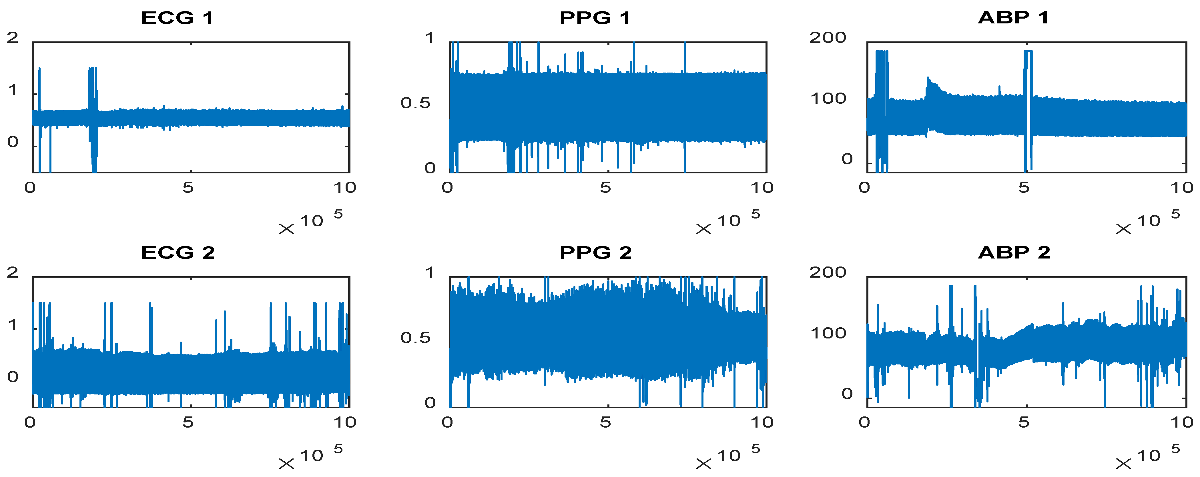
In the next stage, the ECG, PPG, and ABP data were subjected to the low-frequency wavelet technique to remove breathing artifacts or a wandering baseline in the signals (Figure 1) by discarding the last 4 detail wavelet transform coefficients and the approximation coefficient, utilizing the Daubechies 8 mother wavelet with 10 decomposition levels, similar to the approach outlined in [33]. This denoising method was adopted mainly due to a better phase response, computational efficiency, and adaptivity to these biological signals. The whole preprocessing method adopted in this study is resumed in the following lines:

• ECG, PPG, and ABP signal lengths are equal to 2 h.
• In the first step, we remove NaN.
• In the second step, we perform wavelet denoising for low frequency with N = 10 and dB8.
• Window segmentation length is 20 s for N = 292.
• In the final step, QRS-PPG-ABP window segmentation (N = 7057).

Furthermore, the original signal’s mean was added to the one filtered to avoid the loss of inherent offset for the PPG data. By doing so, the morphological and physiological meaning of the Pulse Input Response (PIR) feature will be preserved. PIR is related to the maximum and minimum intensity of the PPG signal within a cardiac cycle. After the 2 signals are cropped into 20 s segments, they are subjected to a threshold. Segments whose minimum or maximum values are below or above the specified threshold are automatically eliminated. In such cases, the lower and the upper thresholds can be computed as

$$threshol{d}_k={\mu }_k+a{\sigma }_k a>0$$

(1)

where a is the adjusted positive scalar of each signal subject. Σ_k and µ_k are the signal k’s mean and standard deviation (STD), respectively. Anytime a signal’s segment is discarded, segments in the same time interval are also discarded to preserve the alignment.

The following procedure was to perform high-frequency wavelet denoising on each 20 s window obtained in the previous step. This process utilized the Daubechies 8 mother wavelet, employed 10 decomposition levels, and applied the soft Rigrsure thresholding approach, with threshold rescaling derived from noise estimates of the first-level coefficients. The Wavelet Toolbox function wden.m in MATLAB was employed to perform this operation.

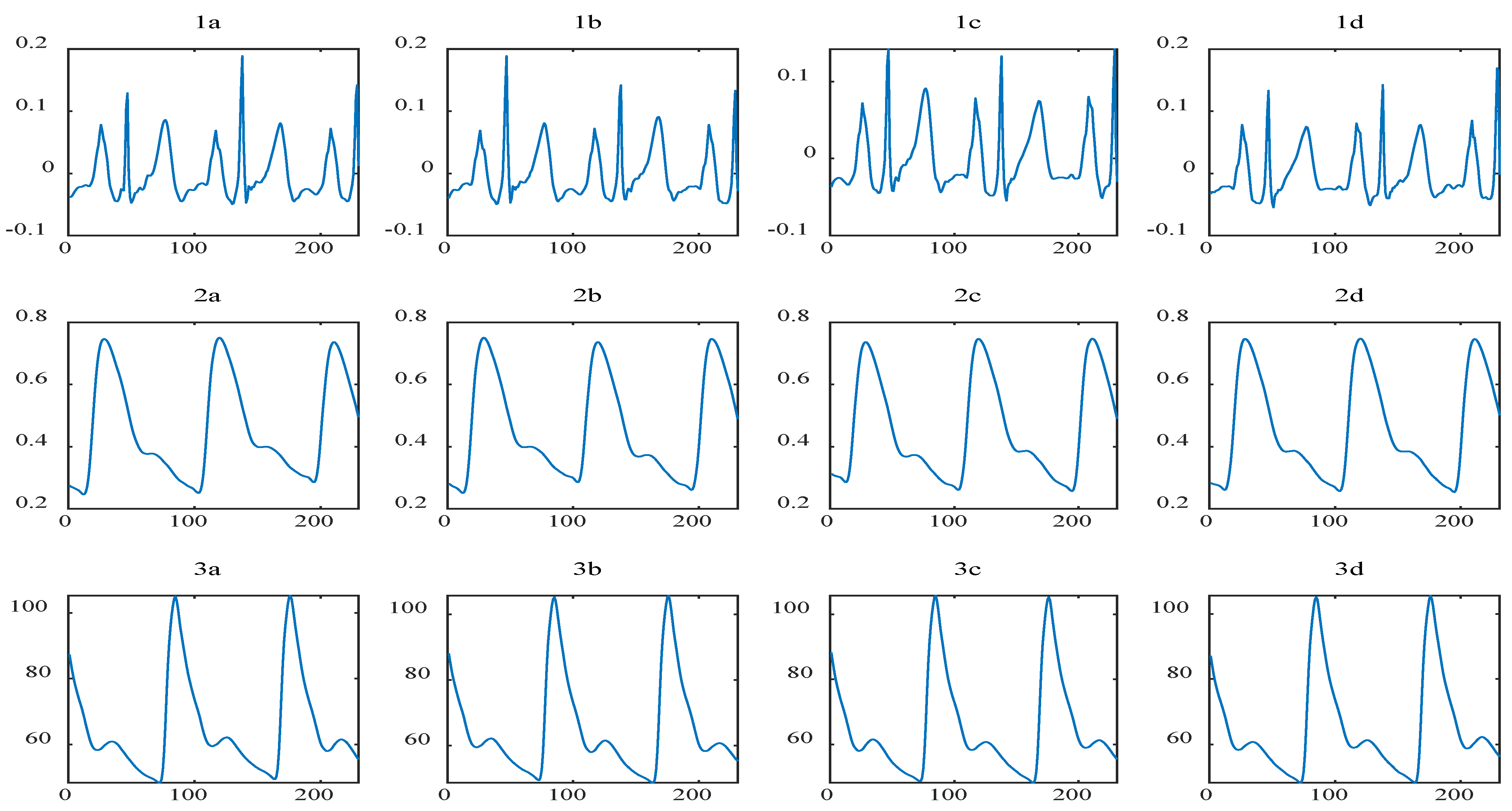
The final processing step involves segmenting 20 s windows of denoised PPG, ABP, and ECG signals into smaller segments with fewer cardiac cycles for our feature extraction functions (see Figure 2). To achieve this, we applied a 4-level wavelet decomposition using the Symlets4 mother wavelet to the ECG signal within each 20 s window. As a result, the R peaks in the ECG signal become highly noticeable and prominent after the reconstruction of the second and third detail coefficients. This phase of our experiment is consistent, as it allows us to precisely determine the time location of the R peaks within each window, thereby exempting the need to detect large P and T waves abnormally. After detecting the R peaks, all three signals were once again segmented into different sets of corresponding intervals. These intervals consist of three PPG pulses: the preceding pulse, the ongoing pulse, and the initial part of the subsequent pulse.

The features necessitating peak detection were obtained using the MATLAB function findpeaks.m, configured with appropriate minimum peak height and minimum peak-to-peak distance settings. The former was determined following Equation (1), while the latter was established based on the typical range of heart rate values, excluding peaks that were in close proximity to subsequent PPG pulses.

4. Feature Extraction

During the extraction section, information from PPG derivatives is taken into account. As Sun, X. et al. mentioned in their study, information from the first and second derivatives of PPG signals is related to atherosclerosis and vascular elasticity, which are the factors that influence BP [34,35], and consequently shows a better correlation with BP inside the blood vessel. Based on this, twenty-one key features are extracted from the PPG signal, its derivative shape, and the time shift between the ECG and PPG wave. All this computation is parameter-based rather than a whole-based extraction of characteristics in the ECG–PPG window linked to BP.

Previous studies have also demonstrated that BP can indeed be deduced from the PTT [36,37], as it is the time interval needed for the arterial pulse to shift from one peripheral to another, which is an indicator of variation in BP. In our model, pulse arrival time (PAT) is then used to measure the targeted pulse transit time since they all have the same amount in representation but differ from the fact that PAT considers a short period during the electrical activation of the heart.

As mentioned previously, PAT is preferred by researchers due to its ease of measurement and its representation of the time interval between the R peak in the ECG and the pulse at the distal end. The time event of ECG and PPG peak (PAT^p), maximum slope point (PAT_d), and diastolic foot (PAT_f) are emphasized in our study, as well as the pulse intensity ratio (PIR), which has also been shown to be inversely proportional to the DBP. And the features are listed as follows:

PPG’s 1st derivative (maximum intensity (dppgH, f₁); period between max and min values (dppgW, f₂); maximum slope point (PAT_d, f₃)), PPG’s 2nd derivative (maximum intensity (ddppgPH, f₄); (ddppgFH, f₅)), peaks (systolic time (ST, f₆); diastolic time (DT, f₇); pulse intensity ratio (PIR, f₈); heart rate (HR, f₉); systolic peak (PAT_p, f₁₀); diastolic peak (PAT_p, f₁₁)), and PPG (inverse of the elapsed time bounded by the PPG maximum and the stationary point: artery stiffness index (ASI, f₁₂), areas under the curve starting from the diastolic foot to the max slop (AUC, f₁₃), from the max slop to systolic peak (AUC, f₁₄), from systolic peak to the stationary point (AUC, f₁₅), and from the stationary point to the next PPG diastolic foot (AUC, f₁₆), and the area under curve ratio: inflection point area (IPA, f₁₇)). IPA evaluates the total peripheral resistance of the blood vessel to blood flow. there may be an inflection point in the trajectory of BP preceding hypertension onset, and the BP will rise relatively faster after the inflection point [38].

$$IPA=\frac{AUC4}{AUC1+AUC2+AUC3}$$

(2)

Our 7057 windows from the processing pipeline were fed into the FeatureExtraction.m function as an input. In this section, four extraction parts took place and windows can be interpreted as samples for the estimated model. The first part allows the extraction of ST, DT, PIR, and PPG where the PPG signal is processed with no peaks and feet detected and 765 rejected. The second part consisted of extracting the first and second derivatives of PPG, AI, ASI, and HR, but the first dPPG peaks and feet failed to be detected, with four rejected. The areas under curves (AUC1, AUC2, AUC3, and AUC4) were extracted in the third part as well as IPA, PAT_d, PAT_f, and PAT_p, but we rejected 23 here. The last and fourth parts allowed us to extract SBP and DBP with an output window of 6265.

5. Deep Learning CNN—Methodology

CNN was performed to quantify features that cause considerable variation in the dataset and eliminate those that are responsible for less variation. This technique is relevant in our study since the number of predictors is reduced and the computing capacity of the model’s training process is improved. Apart from performing CNN, another important step that increased the computation capacity of the training process even more was computing cross-validation tests such as leave-one-out. Since our training procedure was repeated over time, a stepwise multivariate linear regression was also performed to enable us to statistically select features that would work for our model. Having such a large predictor vector may increase computation time, which is why we considered reducing the number of predictors.

Furthermore, in this section, an iterative construction of a regression model was performed and involved choosing predictors or features that are utilized in the final model. The regression model consists of adding or removing potential explanatory features in succession and testing for statistical significance after each iteration. The p-value (with predefined threshold = 0.05) of an F-statistic test was computed and compared to measure the likeliness of having a null coefficient. The latter was computed based on the least square technique. The linear regression model could estimate the systolic BP and diastolic BP values.

$$SBP={\alpha }_0+{\alpha }_1{f}_1+{\alpha }_2{f}_2+\cdots +{\alpha }_n{f}_n$$

(3)

$$DBP={\beta }_0+{\beta }_1{f}_1+{\beta }_2{f}_2+\cdots +{\beta }_n{f}_n$$

(4)

During our experiment, the deep learning method was carried out for the measurements. We hope that deep learning will reduce error rates as a result of these measurements. DeepPhys [39] provides a visualization of physiological information in videos using convolutional attention networks. Eighteen participants from DeepPhys were recorded with a VF0800 camera, equipped with an Intel RealSense by Intel corporation in Santa Clara, CA, USA. The average age of the participants is 37, both men and women were recruited. Videos with 1920 × 1080-pixel resolution were registered with a 24 fps frame rate in 24-bit RGB color. A FlexComp Infiniti was used to evaluate gold-standard physiological signals and the blood volume pulse (BVP). The details of the hyperparameters used are shown in

Table 1. Hyper-parameters used in this work.

Hyper-Parameter	Value
Optimizer	Adam
Weight	ImageNet
Metrics	Accuracy
Epoch	30
Batch size	32
Drop out	20%
Number of hidden units in layer	128

.

The algorithm processes RGB or infrared videos and can accurately obtain heart rate. PhysNet’s main purpose is to use a spatiotemporal network for rPPG signals from videos and extract spatial and temporal hidden features simultaneously from raw face sequences, as in [40]. Then, it compares rPPG signals with Ground Truth ECG values. The method makes peak detection to find the interbeat interval for average HR and HR variability. It creates linear models capable of predicting SBP and DBP values (Figure 3). Root mean square error (RMSE) is the STD of the prediction errors called residuals. Residuals can be measured by how far data points are from the regression line. The RMSE value is a measure of how far these residues have spread. The RMSE value can be calculated as follows:

$$RMSE=\sqrt{\frac{\sum _{i=1}^N(Predicte{d}_i-\mathrm{A}\mathrm{c}\mathrm{u}\mathrm{a}{l}_i{)}^2}{\mathrm{N}}}$$

(5)

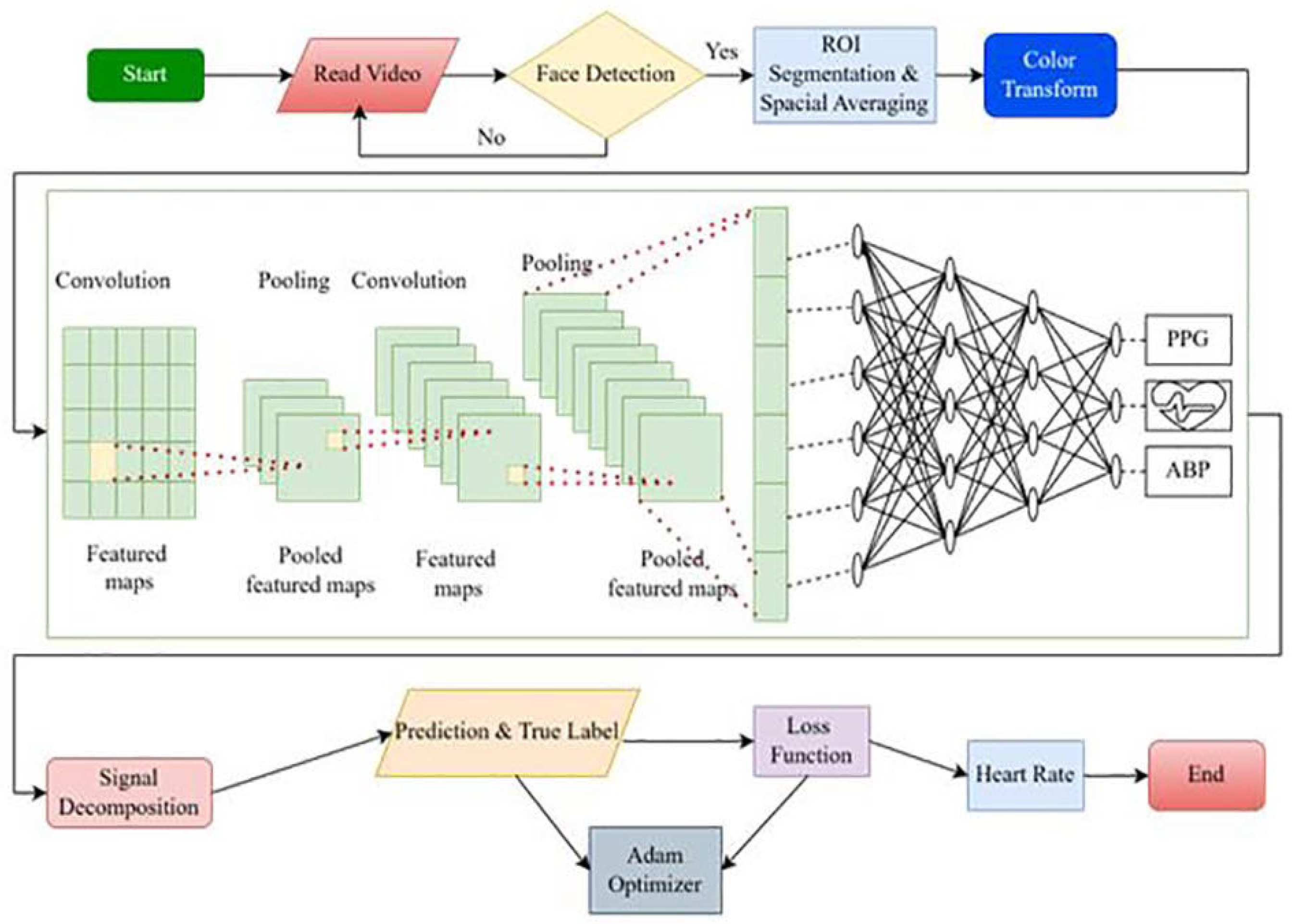
Acquisition of video data: this process initiates with the acquisition of video data, wherein the facial region of a subject is aimed to be captured continuously over a certain period of time. The quality and clarity of the video are pivotal, ensuring the algorithms can effectively discern features necessary for subsequent analyses.

Face detection loop: the face detection mechanism is subsequently employed, where the algorithm attempts to identify the face in the acquired video data. This step is crucial for isolating the region of interest (ROI) in the later steps. If a face is successfully detected, the process proceeds to the ROI segmentation. If the algorithm fails in face detection, it enters into a loop, continually attempting to detect the face until successful.

ROI segmentation and spatial averaging: upon successful face detection, ROI segmentation and spatial averaging are conducted to localize and focus on the facial region relevant to heart rate and blood pressure estimation. This involves delineating the region where PPG signals can be extracted effectively and then utilizing spatial averaging to enhance the signal quality by reducing noise and irrelevant spatial variations.

Color transformation and CNN model application: following the segmentation, color transformation is applied to the ROI, optimizing the visual data for the extraction of hemodynamic signals. The transformed data are then input into the convolutional neural network (CNN) model. The CNN model is designed and optimized using specific parameters, such as utilizing the Adam optimizer, pre-training weights with ImageNet, and gauging performance via accuracy metrics. The training process encompasses 30 epochs, a batch size of 32, a dropout rate of 20%, and utilizing 128 hidden units per layer.

Classification and parameter optimization: the CNN model, now processed with the color-transformed ROI, endeavors to classify and estimate the PPG, ABP, and HR of the subject. This step involves the intricate and nuanced utilization of deep learning algorithms to sift through the spatially averaged and color-transformed data, identifying patterns and features relevant to the accurate classification and estimation of the physiological parameters of interest.

Output and further analysis: lastly, the classified and estimated PPG, ABP, and heart rate serve as the output, potentially utilized for further analysis or real-time monitoring applications. These data, derived cuffless, present opportunities for non-invasive monitoring in various contexts, offering insights into cardiovascular health without the necessity for traditional, more invasive methods.

6. Result

6.1. Dimensionality Reduction

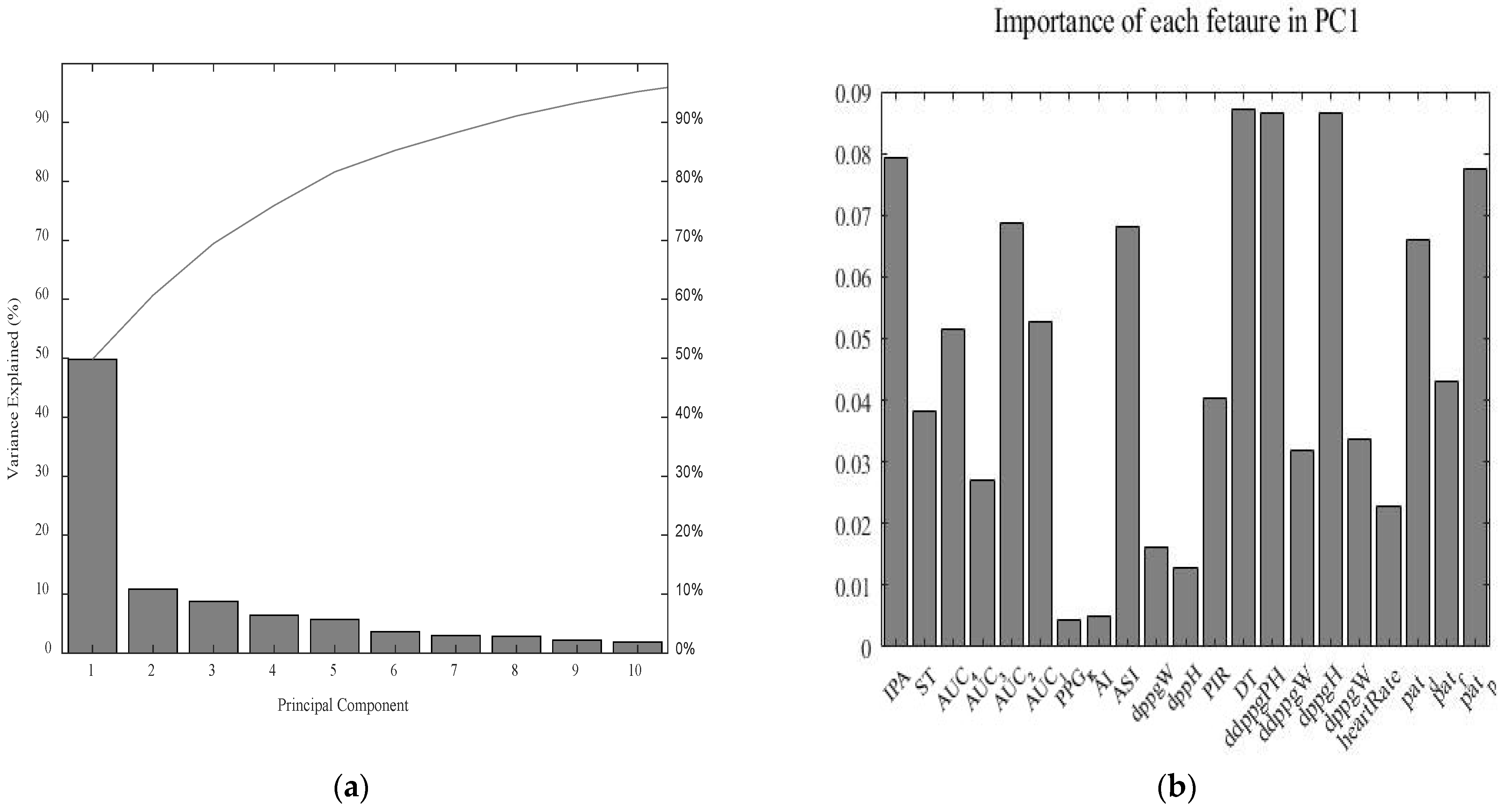
Principal component analysis (PCA) was conducted to find the proportion-of-variance (pov), explained curve, and scree plot which indicates the number of dimensions with the most variance to be selected. When considering the scree plot for the entire spectrum of the sample, it was observed that only half (50%) of the variance is explained by the component, as depicted in (Figure 4a). Moreover, when we analyzed the contribution of every feature to this component, we realized that every feature approximately contributes the same amount to it, as depicted in (Figure 4b). Therefore, it is too difficult to conclude any feature selection and data reduction based on these observations. As a matter of fact, for a model to be estimated accurately, it is practical to focus on feature reduction based on the principal component when some features are dominated by others in regard to the variance explained, which is not the case here.

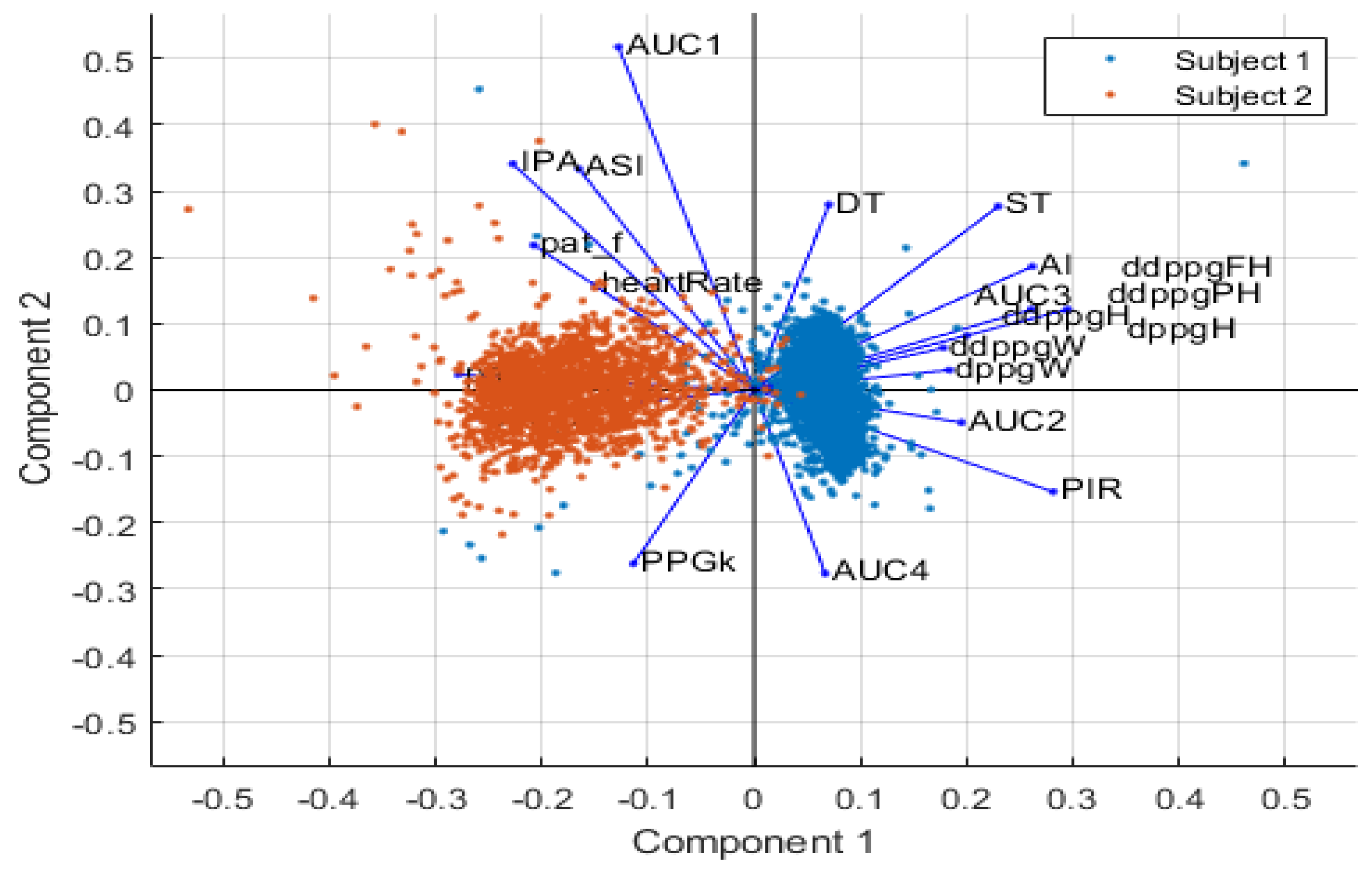
Nevertheless, after projecting the dataset on the plane defined by the two first principal components (the plane explained by the most variance), as depicted in Figure 5, it is clear that the samples cluster into two different groups. And, obviously, these groups correlate to the two different sources of data that are considered in this study. What we can infer from this is that the principal source of variance within the dataset is the origin of the samples. Such a link between the samples and the source of variance was expected since the data from MIMIC-II were acquired in different environments from different subjects with different health conditions and physiological characteristics. The extracted features would have been our main source of variance if a larger dataset had been utilized from larger patients.

From Figure 5, the X-axis represents the projection on the PC1 axis in association with PC1. The axes demonstrate the principal component scores. First, we can see that samples from subject 1 and subject 2 are located closer to each other, which indicates that they all belong to the same species of subject. Secondly, it can be noticed that subject 2 has relatively lower PC1 scores [−0.5, 0], whereas subject 2 has rather higher PC1 scores [0, 0.5]. Finally, we can see that features such as DT, ST, AI, AUC2, ddppgFH, ddppgPH, dppgH, AUC3, PIR, and AUC4 are in the same direction as PC1; consequently, they are positively correlated with PC1, which implies a positive association.

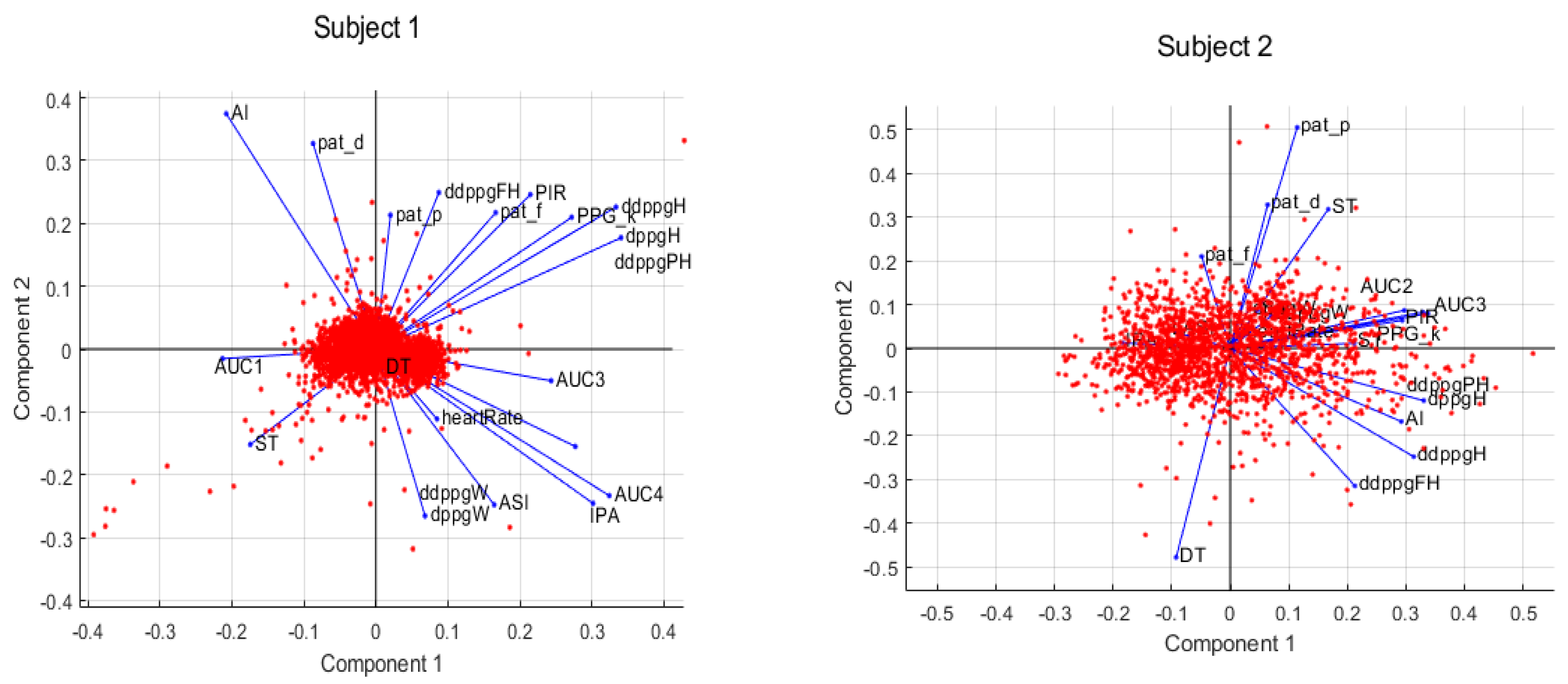
When the subsets of each subject are analyzed separately into their own plane, we can note that subject 2 expressed more variation than subject 1 (Figure 6). This was expected because subject 2’s PPG signal’s amplitude varied more across the samples (Figure 1). Most of the features are positively correlated for each subject (Figure 6), which means they have relatively higher scores in PC1. When feature weight analysis was performed on the first principal component, it was observed that each feature explained similar variance among subsets; for example, features like the first and second derivative of PPG maximum intensity (dppgH, ddppgPH) are likely to explain the same amount of variance in the two subsets, but AUC2 explained different amounts of variance in subject 1 and subject 2.

Analyzing the weight distribution on the first principal component of the subset (depicted in Figure 4b) allows us to grasp the similarity in variance explained by individual features across subjects. Notably, features DT, ddppgPH, and dppgH appear to explain a similar relative variance in the subsets. Additionally, it is pertinent to observe that features such as AI, PPG_k, and AUC1 do not substantially elucidate variance in either subset; however, when considering the entire dataset, their explanatory power increases. These features exhibit a stronger correlation with the variance stemming from disparities among patients.

6.2. Stepwise Multivariate Linear Regression

A total of 57 datasets were employed as training sets for regression purposes, the following models were tested: (i) incorporating features from both subjects’ signals, (ii) exclusive use of subject 1’s data, and (iii) exclusive use of subject 2’s data. Subsequently, the corresponding models underwent evaluation, using all available windows from (i) subject 1 and 2, (ii) subject 1 alone, and (iii) subject 2 alone as testing sets. This evaluation employed leave-one-out cross-validation.

Furthermore, the models built with training sets that contained information from only one of the subjects were also assessed using the data of the other subject. This assessment aimed to confirm the presence of any bias within the models, specifically whether they exhibited inferior performance when estimating SBP and DBP values for the subject not included in their training set. The results demonstrated were worse when estimating SBP and DBP values of the subject excluded from the training set (

Table 2. RMSEs, standard deviation (STD), and MAEs of the linear regression models with alternating training and testing sets.

Training Set	Testing Set	Systolic Blood Pressure (mmHg)			Diastolic Blood Pressure (mmHg)
		MAE	STD	RMSE	MAE	STD	RMSE
Subject 1	Subject 2	13.32	10.87	17.00	9.20	6.33	11.18
Subject 2	Subject 1	36.80	7.00	37.45	22.40	3.62	22.70

). In each of these evaluation scenarios, metrics such as the mean absolute error (MAE), standard deviation (STD), and root mean Squared error (RMSE) were computed to quantify performance.

The function trapz.m in MATLAB was used to extract the features that were placed under the PPG curve based on the trapezoidal rule approximation method by integrating the input curve between specified points numerically. As described in the method section, the windows that were generated previously from the signals are fed into the FeatureExtraction.m function as an input, and we implemented functions to extract features at various steps. At each step, these windows pass through quality control, and if they do not carry any interpretable signal, then they are rejected, which means the well-documented features of each signal are absent. This is a crucial advance in our implementation because, even if we tried to remove maximum noise and large amplitude artifacts, there may remain some low-amplitude artifacts that corrupt the samples.

In

Table 3. Rejected or not rejected feature during the stepwise linear regression with subsets. ‘X’ means rejected or discarded and ‘√’ means ‘not rejected’.

Features	Subjects 1 and 2		Subject 1 Only		Subject 2 Only
	SBP	DBP	SBP	DBP	SBP	DBP
(dppgH)	X	X	√	√	X	√
(dppgW)	√	√	√	√	X	√
(PATd)	√	√	√	√	X	X
(ddppgPH)	X	X	X	X	X	X
(ddppgFH)	√	√	X	√	X	X
(ST)	√	√	X	X	X	X
(DT)	√	√	√	√	√	√
(PIR)	X	√	√	√	X	√
(HR)	√	√	√	√	X	X
(PATp)	√	√	√	√	√	X
(PATf)	X	X	X	√	X	X
(ASI)	√	√	√	√	√	√
(AUC1)	√	√	√	X	√	X
(AUC2)	√	√	√	√	√	X
(AUC3)	√	√	√	√	X	X
(AUC4)	√	√	√	√	X	√
(IPA)	√	√	√	√	√	X
(AI)	√	√	√	√	√	√
(ddppgW)	√	X	√	√	X	√
(PPGk)	X	X	√	X	X	√
(ddppgH)	X	X	√	X	√	X

, the features excluded or chosen by our stepwise linear regression algorithm are displayed, and their selection varies depending on the training dataset and the target variable, either SBP or DBP. Notably, when focusing on subject 2’s subset, we observed a larger number of features that were considered statistically insignificant for the regression model. This observation might be attributed to the high variance shown by this patient, as previously mentioned, in contrast to the data from subject 1.

We consistently observed that feature ddppgPH was removed in all training sets, indicating a significant likelihood of its model coefficient being zero. This suggests that this feature may not exhibit as strong a correlation with both SBP and DBP as the other features. Additionally, the parameter PAT_f is consistently excluded from the predictor vector across all training sets, except when estimating DBP with subject 1’s dataset. This further suggests that this particular feature may not be as strongly correlated with blood pressure as the other features. Based on our sample data, the features that appear to exhibit the highest correlation with blood pressure values are those that were retained without removal when the model was applied to each training set. These features include DT, ASI, and AI, respectively.

7. The Estimation Models Discussion

In

Table 4. Calculated RMSE and RMSE of the linear models for each training subset with corresponding SBP and DBP variance.

Training Set	Systolic BP		Diastolic BP
	RMSE (mmHg)	Variance (mmHg2)	RMSE (mmHg)	Variance (mmHg2)
Subject 1 and 2	7.5	78	3.83	52.1
Subject 1 only	4.40	38.49	1.5	6.6
Subject 2 only	10.60	170.2	5.9	51.49

, the regression RMSE values are presented. These values indicate how well the linear regression models fit our datasets. Specifically, subject 1’s model displays the lowest RMSE values, with 4.4 mmHg for SBP and 1.5 mmHg for DBP, indicating a stronger linear correlation among their features. In contrast, subject 2’s models display the highest RMSE values among the 3 datasets, measuring 10.60 mmHg for SBP and 5.9 mmHg for DBP, showing a weaker linear correlation among their features compared to subject 1’s model. As a result, the models that combine information from both subjects fall in between the RMSE values of 7.5 mmHg for SBP and 3.83 mmHg for DBP.

Furthermore, it is worth highlighting that we observed smaller RMSE and STD values in the models designed for estimating DBP in contrast to those for SBP. This discrepancy may be attributed to the lower variance in DBP. A similar trend is observable when comparing the RMSE and STD of the fits between subject 1’s subset and subject 2’s, where the latter shows larger values due to lower data quality and more varied signal (Figure 1).

The leave-out-cross validation was used to assess the model’s capacity for generalization to an independent dataset, as displayed in

Table 5. Cross-validation of the linear models with the calculated RMSEs, standard deviation (STD), and MAEs. Compared with other works. Subject (S). Not provided (NP).

Works	Systolic Blood Pressure (mmHg)			Diastolic Blood Pressure (mmHg)
	MAE	STD	RMSE	MAE	STD	RMSE
CNN-BiLSTM in [31]	7.849	NP	11.50	4.418	NP	6.52
GRNN in [41]	5.36	NP	5.54	3.28	NP	3.45
KNN in [42]	6.52	NP	NP	NP	5.20	NP
ML in [43]	8.64/9.45	NP	NP	18.20/8.13	NP	NP
Proposed model (S1 and S2)	4.70	7.60	7.51	2.01	3.90	3.90
S1 only	3.30	3.08	4.52	1.10	1.12	1.56
S2 only	6.56	8.4	10.71	3.48	4.80	5.91

. It is important to note that models derived from the two subjects are limited by the number of subjects used in the data, making it unlikely for the models to accurately estimate the SBP and DBP of subjects other than subjects 1 and 2. Still, our model shows lower MAE and STD values when compared with the parameter-based CNN and Bidirectional Long Term Memory model performed in [31] with MAE (7.849 mmHg), RME (11.503 mmHg), MAE (4.418 mmHg), and RME (6.525 mmHg) for the SBP and DBP, but without any feature extraction. Moreover, we also compared our results with studies using machine generalized regression neural networks (GRNNs) developed on the MIMIC II database in [41], K-nearest neighbors’ algorithm (KNN) by Fati, S.M et al. [42], and the machine learning method implemented by Simjanoska et al. in [43], shown in Table 5.

The models that exclusively utilize information from subject 1 show lower MAE, STD, and RMSE values when compared with those based on subject 2. This difference shows the former models’ enhanced ability to estimate subject 1’s SBP and DBP compared to the latter models’ performance in predicting subject 2’s values. The variability in subject 2’s signals is a probable factor influencing the accuracy of the models’ predictions. The performance of the models using data from one subject when applied to the other subject’s data was also assessed, as shown in Table 5. Notably, the MAE, STD, and RMSE values are greater in this scenario in comparison to the error values reported in Table 4 and Table 5. These models are specifically tailored to each subject due to the training set relying on one of the subjects. Therefore, the accuracy decreases when predicting the SBP and DBP of the other subject.

Limitations and Future Recommendations

Based on the experiment conducted in this study, it is crucial to emphasize that the quality of the fit and, consequently, the determination of which features are statistically significant in the regression depend on the set of features initially included in the stepwiffit.m function algorithm. The regression algorithm works to find a locally optimal fit. This implies that had we chosen a different combination of features for the initial model instead of starting with an empty vector, we would have guaranteed global optimal fit [44]. Moreover, our observations are based on a small sample of two subjects. Therefore, the generalization of our findings to a broader population is limited. The features we have identified as significant might have been different if the dimension of the training had encompassed data from diverse individuals with varying physiological characteristics and health statuses. We foresee that the accuracy of our model could be enhanced by incorporating additional physiological factors such as age, height, and weight, as these variables can influence blood pressure. PPG represents an optical sensor measurement technique employed in the prevention of CVDs. We anticipate a forthcoming trend in the development of optical biosensor algorithms, enabling the utilization of intracellular, stationary, and time-dependent information for disease diagnosis [45].

8. Conclusions

Our MATLAB implementation allowed us to successfully extract vital blood pressure-related features from the PPG’s shape and the time shift concerning the ECG, as well as SBP and DBP values derived from the ABP waveform. Analysis of the performed CNN revealed that the main source of variance within the dataset originated from the subjects themselves, indicating that the subject’s identity was the most significant factor contributing to the variance. There was no clear predominance of variance attributed to, or explained by, any specific feature; therefore, no dimensionality reduction was performed based on these features.

Our estimation models were developed using a stepwise multivariate linear regression approach, which facilitated the elimination of certain features based on their statistical significance in the regression. As expected, models trained with data from a single subject tended to overestimate their performance when applied to samples from the same subject. The results of our cross-validation demonstrated improved MAE and STD values compared to those reported in the literature, primarily due to the more limited dimensions of our dataset. This led to results with smaller MAE and STD; however, these outcomes were somewhat overfitted to our specific pair of subjects. The limited amount of interpretable data at our disposal raises questions regarding the generalizability of our models to data from other subjects. On a positive note, we have confidence in the adaptability of our preprocessing and feature extraction pipeline to different datasets.