Article

Fault Diagnosis Method for Railway Turnout with Pinball Loss-Based Multiclass Support Matrix Machine

School of Electronic and Information Engineering, Tongji University, Shanghai 201804, China
*
Author to whom correspondence should be addressed.
Appl. Sci. 2023, 13(22), 12375; https://doi.org/10.3390/app132212375
Submission received: 9 October 2023 / Revised: 8 November 2023 / Accepted: 13 November 2023 / Published: 15 November 2023
(This article belongs to the Special Issue Transportation Planning, Management and Optimization)

Abstract

:
The intelligent maintenance of railway equipment plays a pivotal role in advancing the sustainability of transportation and manufacturing. Railway turnouts, being an essential component of railway infrastructure, often encounter various faults, which present operational challenges. Existing fault diagnosis methods for railway turnouts primarily utilize vectorized monitoring data, interpreted either through vector-based models or distance-based measurements. However, these methods exhibit limited interpretability or are heavily reliant on standard curves, which impairs their performance or restricts their generalizability. To address these limitations, a railway turnouts fault diagnosis method with monitoring signal images and support matrix machine is proposed herein. In addition, a pinball loss-based multiclass support matrix machine (PL-MSMM) is designed to address the noise sensitivity limitations of the multiclass support matrix machine (MSMM). First, the time-series monitoring signals in one dimension are transformed into images in two dimensions. Subsequently, the image-based feature matrix is constructed. Then, the PL-MSMM model is trained using the feature matrix to facilitate the fault diagnosis. The proposed method is evaluated using a real-world operational current dataset, achieving a fault identification accuracy rate of 98.67%. This method outperforms the existing method in terms of accuracy, precision, and F1-score, demonstrating its superiority.

1. Introduction

The intelligent maintenance of railway equipment has garnered increasing attention as a way to enhance sustainable transportation and manufacturing [1,2]. As an essential topic in prognostics and health management (PHM), fault diagnosis can help reduce the workload for inspectors and enhance the efficiency of traditional regular inspections [3,4]. Intelligent fault diagnosis technology applications can concurrently enhance the reliability and transportation efficiency of rail systems. With the timely and accurate diagnosis and repair of faults, railway transportation can better meet the demands of industrial supply chains, ensuring the safety and timely delivery of goods.
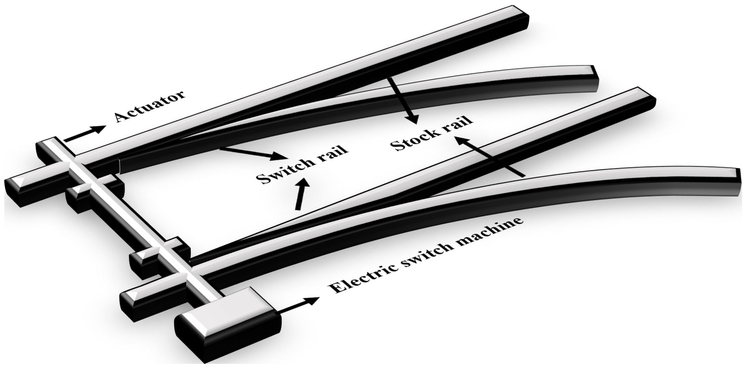
The traffic planning of railways primarily relies on controlling turnouts. Turnouts are essential elements of railway systems because they allow track switching and enable trains to travel on different routes [5,6]. The turnout switch machine system comprises stock rails, switch rails, and switch machines [7,8], as shown in Figure 1. However, these turnouts may encounter failures due to various factors, disrupting the transportation process. Therefore, the proper functioning of turnouts is crucial to maintaining the safety and efficient operation of trains, as well as to enhancing transportation efficiency.
Currently, there is a growing focus on data-driven intelligent fault diagnosis research in railway turnout. The primary approach to diagnosing faults in railway equipment relies on the use of train monitoring data [9]. Turnout fault diagnosis methods generally involve data acquisition, feature extraction, and pattern recognition [10,11]. From a feature construction perspective, these methods can be divided into three categories: pattern recognition, distance measurement, and deep learning methods. Pattern recognition methods generally rely on statistical or signal-processing-based indicators [12]. Ji et al. [3] developed a fault diagnosis model for rail transit turnouts by extracting statistical features through curve segmentation. Sun et al. [13] introduced fractional calculus into wavelet packet decomposition energy entropy to represent switch fault characteristics. Chen et al. [14] proposed an energy-based threshold wavelet method for turnout fault diagnosis. Although these methods achieve a satisfactory performance, the extracted features lack interpretability, which affects their application in practical engineering. The method employed for the on-site detection of railway equipment involves the interpretation of monitoring data curves through the visual inspection of corresponding images. Images are better suited for processing curve data because they contain more detailed structural information, thereby aligning with real-world scenarios. However, the aforementioned methods reshape their structures into vectors to fit the model, disregarding the spatial structure of the original time-domain signal, resulting in information loss. By contrast, the distance measurement methods aim to identify the fault by evaluating the distance between the test and standard curves [15]. Zheng et al. [16] used the Hausdorff distance to calculate the similarity of an action power curve and built a fault-detection model. Huang et al. [17] adopted the Fréchet distance to measure the similarity of the current action curve to identify normal versus abnormal data. These methods facilitate fault diagnosis by assessing distances between curves, demonstrating notable interpretability. However, a marked dependence on standard curves renders these methods infeasible for broad generalization.
Deep learning with automatic features has experienced rapid development in recent years [5,18,19,20]. Guo et al. [21] developed an unsupervised railway turnout fault detection method using a deep autoencoder. Li et al. [22] proposed an autoencoder-based fault diagnosis method for railway turnout. Lao et al. [23] proposed a dual-scale neural network-based fault diagnosis method to solve the data scarcity problem in labeled fault data. The method used a one-dimensional vibration signal as the input. These methods effectively mitigate the limitations associated with expert experience. However, the data processing or model in these studies ignores the structural information of the time series data, resulting in the loss of spatial structure-related information and subsequently impacting the method’s performance [24,25].
In recent years, matrix-based machine learning has gained attention as a pattern recognition method that utilizes matrix data as inputs [26]. Relative to vector-based pattern recognition and deep learning methods for railway turnout fault diagnosis, matrix-based machine learning can preserve the structural information of the time series data. Additionally, unlike distance measurement methods that heavily rely on standard curves, this approach is not constrained by predefined curves, enhancing its adaptability to diverse datasets. Luo et al. [27] introduced a support matrix machine (SMM) that employs the hinge loss, Frobenius norm, and kernel norm to integrate the structural information of the input matrix. Support vector machine (SVM) is designed for vector inputs. However, when dealing with matrix data, it is necessary to reshape the matrix into a vector, which may result in the loss of structural information. In contrast, SMM operates directly on matrix data, preserving the inherent structural information. SMM extends the concept of SVM to matrices and utilizes the hinge loss, Frobenius norm, and kernel norm to integrate the structural information of the input matrix. This enables SMM to capture the dependencies and relationships between different elements of the matrix. Subsequently, many improved SMMs have been developed to enhance performance in various classification scenarios. Li et al. [28] presented a least squares interactive SMM to improve computational efficiency and address the SMM problem in multi-quadratic programming. Zheng et al. [29] built upon the objective function that combines multiclass hinge loss and regularization terms. However, these models tend to be sensitive to noise, which is attributed to the integration of hinge loss functions. Fault diagnosis is a multiclassification problem. Datasets for industrial scenarios generally contain a lot of noise. To solve the limitation in noise-sensitivity and enhance the performance of MSMM for fault diagnosis problems, we design a pinball loss function-based [30] MSMM called the PL-MSMM. We then employ PL-MSMM to diagnose turnout faults. The main contributions of this study can be summarized as follows:
  • A multiclass classifier with a pinball loss function is designed, namely PL-MSMM. Industrial datasets often contain noise. This classifier is better equipped to handle noisy data, making it well-suited for real-world industrial scenarios.
  • A railway turnouts fault diagnosis method with monitoring signal images and the designed PL-MSMM is proposed. It does not rely on the standard curve and takes into account the spatial structure of the time series monitoring signal, giving it better generalizability and performance.
  • The proposed method is validated using a real-field current dataset. The experimental results demonstrate its efficiency as a turnout fault diagnosis framework in practical scenarios.
The remainder of this paper is structured as follows. The proposed classifier is presented in Section 2. The proposed diagnostic method is described in Section 3. The testing of the proposed method using field data is discussed in Section 4. Finally, Section 5 concludes the paper and provides recommendations for future work.

2. Classifier Design

2.1. Brief Review on Support Matrix Machine

2.1.1. Support Matrix Machine

To effectively preserve the row and column structural information of the original input matrix, Luo et al. [27] proposed an SMM that could retain matrix structure information. Given a matrix sample set X i = 1 n , the ith input matrix sample X i R p × q , and corresponding label y i , the SMM’s optimization problem can be expressed as (1), whose objective function comprises the hinge loss, kernel norm, and Frobenius norm:
min W , b , ξ 1 2 tr W T W + τ W * + C i = 1 n ξ i s . t .   y i tr W T X i + b 1 ξ i a n d   ξ i 0   f o r   i { 1 , 2 , , n } ,
where W R p × q denotes the regression coefficient matrix and tr ( W T W ) represents the trace of the matrix. To preserve the relevant matrix structural information, we consider the dependence of the regression matrix W , which can be expressed as rank W . The kernel norm W * denotes the best convex approximation function of rank W . τ is a kernel norm constraint parameter. C denotes a regularization parameter; finally, ξ represents a sequence of slack variables utilized for the hinge loss.

2.1.2. Multiclass Support Matrix Machine

To handle multiclassification problems, there are some methods with which to extend SMM to support multiclass classification tasks with matrix-form data [29]. The objective function of the multiclass SMM can be defined as follows:
min W , ξ 1 2 W F 2 + τ j = 1 k W j * + C n i = 1 n ξ i , s . t .   Δ y ^ i , y i + W , δ Ψ X i , y ^ i , y i ξ i a n d   ξ i 0   f o r   y ^ 1 , y ^ 2 , , y ^ n Y n ,
where W R p × q × k denotes the tensor form of the regression parameter, W F is the Frobenius norm of W , W F 2 = tr W T W . ξ denotes a sequence of slack variables for the hinge loss. Δ is the Hamming loss function. δ Ψ X i , y ^ i , y i denotes the difference of feature mappings between an arbitrary label y ^ i and the ground truth label y i for input matrix X i .

2.2. Brief Description of the Pinball Loss Function

In the hinge loss function—which punishes only misclassified points—the pinball loss is related to the quantile distance and also punishes correctly classified points [30]. The pinball loss can be expressed as follows:
L p u = u , u 0 p u , u < 0    ,
where u denotes the difference between the predicted and true labels of the model samples, and p 0 , 1 denotes a quantile that can be regarded as a hyper-parameter that controls the degree of punishment of the loss function for different errors. This can improve the classifier’s insensitivity to noisy data.

2.3. Proposed PL-MSMM

In this study, we introduced pinball loss into the multiclass SMM—namely, the PL-MSMM. The PL-MSMM is an anti-noise sensitive matrix form classifier, which effectively handles multiclass fault diagnosis tasks.
Given a k class matrix training dataset X i , y i i = 1 n X , Y , the objective function of the PL-MSMM can be defined as follows:
min W , ξ 1 2 W F 2 + τ j = 1 k W j * + C n i = 1 n ξ i , s . t .   Δ y ^ i , y i + W , δ Ψ X i , y ^ i , y i ξ i a n d   p Δ y ^ i , y i + W , δ Ψ X i , y ^ i , y i ξ i f o r   y ^ 1 , y ^ 2 , , y ^ n Y n ,
where W R p × q × k denotes the tensor form of the regression parameter, W F denotes the Frobenius norm of W , and W j j = 1 k denotes the matrix-form hyperplane of the j th class data. C represents the loss term parameter, and τ is positive values used to constrain the kernel norm. p is the pinball loss parameter, ξ represents a sequence of slack variables for the hinge loss, and δ Ψ X i , y ^ i , y i represents the discrepancy in feature mappings between an arbitrary label y ^ i and the truth label y i for the input X i .
δ Ψ X i , y ^ i , y i = Ψ X i , y ^ i Ψ X i , y i ,
where the feature map Ψ ( X , j ) R p × q × k denotes a sparse tensor with zero elements except for Ψ : , : , j = X .
Equation (4) contains n slack variables. Owing to the multiclass pinball loss and nuclear norm, the optimization problem is non-smooth and non-differentiable. To address this, we can merge n slack variables into a single variable and construct a framework based on the alternating direction method of multipliers (ADMM). The ADMM methodology, renowned for its adeptness in handling non-smooth and non-differentiable optimization problems, emerges as a suitable alternative for effectively navigating the intricacies inherent to the problem at hand [27].
By exploiting the independence of each estimated label, the n slack variable ξ i in (4) can be reduced to a single slack variable ξ , ξ = 1 n i = 1 n ξ i , which denotes the equivalent upper bound of the inequality under all constraints. This allows us to rewrite the objective function as follows:
min W , ξ 1 2 W F 2 + C ξ + τ c = 1 k W c * s . t .   1 n i = 1 n Δ y ^ i , y i + W , δ Ψ X i , y ^ i , y i ξ a n d   p 1 n i = 1 n Δ y ^ i , y i + W , δ Ψ X i , y ^ i , y i ξ f o r   y ^ 1 , y ^ 2 , , y ^ n Y n .
The number of slack variables in (6) can be reduced to one by increasing the number of constraints on Y n , all the constraints sharing a single slack variable ξ . By rewriting the objective function in an unconstrained form, the above equation can be expressed as follows:
min W 1 2 W F 2 + τ c = 1 k W c * + max y ^ 1 , , y ^ n Y n C 1 n i = 1 n Δ y ^ i , y i + W , δ Ψ X i , y ^ i , y i , p 1 n i = 1 n Δ y ^ i , y i + W , δ Ψ X i , y ^ i , y i .
The objective function in (7) comprises three convex terms—that is, the nuclear and Frobenius norms that satisfy the triangle and homogeneity properties, respectively, the third term being the maximum value of a set of linear functions, making it convex. Consequently, the objective function in (7) is convex but non-differentiable and non-smooth. The ADMM framework can be used to address convex optimization problems by decomposing the objective function into subproblems that are easier to optimize [31,32].
The optimization problem in (7) can be viewed as a combination of the loss function and regularization term. In other words, the objective function comprises two parts without any coupled constraints. By introducing a new variable Z = W and changing the variable W in the second part to Z while adding new constraint conditions, the ADMM framework can be used to handle both parts separately. The original problem can be rewritten as follows:
min W , Z P W + Q Z s . t .   W Z = 0 ,
where Z R p × q × k denotes the additional variable that decomposes the original problem into two subproblems.
P W = max y ^ 1 , , y ^ n Y n C 1 n i = 1 n Δ y ^ i , y i + W , δ Ψ X i , y ^ i , y i , p n i = 1 n Δ y ^ i , y i + W , δ Ψ X i , y ^ i , y i ,
Q Z = 1 2 Z F 2 + τ c = 1 k Z c * ,
where P W denotes the loss function and Q Z includes the regular term. The augmented Lagrangian method can be applied to solve (8):
L W , Z , Λ = P W + Q Z + Λ , Z W + ρ 2 Z W F 2 ,
where Λ denotes the Lagrangian multiplier and ρ > 0 denotes the hyper-parameter.
Then, we can decompose the optimization problem into two subproblems: W and Z . The ADMM algorithm minimizes and alternates by iteratively solving and then updating the Lagrange multiplier multipliers Λ accordingly.
Z t + 1 = arg min Z L Z , W t , Λ t ,
W t + 1 = arg min W L Z t + 1 , W , Λ t ,
Λ t + 1 = Λ t + ρ Z t + 1 W t + 1 ,
where t and t + 1 denote the t-th and t + 1 -th iterations, respectively. The derivations of Z t + 1 and W t + 1 are discussed next.

2.3.1. Solving Subproblem Z

First, the objective function with respect to Z can be minimized by fixing W . L Z can be defined as the aggregate of all Z -related terms in (11), as follows:
min Z L Z = Q Z + Λ , Z + ρ 2 Z W F 2 .
Equation (15) can be solved by minimizing L Z . As L Z is a non-differentiable convex function, its sub-gradient can be calculated as follows:
L Z Z j = Z j + τ Z j * + λ j + ρ Z j W j ,
where Z j , W j , and λ j denote the matrix-form hyperplanes of the j-class data for Z , W , and Λ , respectively. Z j * denotes the sub-gradient of the kernel norm.
The optimal solution can be represented as a singular value-thresholding operator [29], as follows:
Z j * = 1 1 + ρ D τ ρ W j λ j ,
where D τ denotes the singular value-thresholding operator.
D τ A = U Σ τ V T ,
where Σ τ = diag σ 1 ( A ) τ + , , σ r ( A ) τ + .

2.3.2. Solving Subproblem W

Similarly, we can fix Z and minimize the part of (11) related to W , denoted as L W , as follows:
min W L W = P W + Λ , W + ρ 2 Z W F 2 .
Equation (18) is the convex sum of the loss term P W with the linear and square functions.
J X i , y ^ i , y i : = 1 n i = 1 n Δ y ^ i , y i + W , δ Ψ X i , y ^ i , y i .
The sub-gradient of P W can be expressed as follows:
P W = C n i = 1 n δ Ψ X i , y ^ i , y i , J p J p C n i = 1 n δ Ψ X i , y ^ i , y i , J < p J    ,
where
y ^ i = arg max y Y J X i , y , y i , p J X i , y , y i .
Thus, the sub-gradient of L W with respect to W is
L W = P W Λ ρ Z W .
Then, the gradient descent method can be used to update W , as follows:
W t + 1 = W t α L W ,
where α denotes the learning rate.
Ultimately, the Lagrangian multiplier can be refreshed as follows:
Λ t + 1 = Λ t + ρ Z t + 1 W t + 1 .

3. Proposed Diagnosis Method

In this study, a novel fault diagnosis method for railway switches is introduced using the PL-MSMM. The proposed method used the A-phase current signals of the railway switch as its input, outputting the corresponding fault type of the switch. The framework for the railway switch fault diagnosis is shown in Figure 2.
  • Data preprocessing: The module’s inputs are A-phase current signals in time series. The preprocessing content includes data cleaning, normalization, and division of reasonable training and testing datasets.
  • Feature matrix generation: This module employs image representation for curve data to align with domain-specific knowledge. The images are transformed into the feature matrix as the modeling input.
  • Supervised learning: This module utilizes the PL-MSMM, as designed in Section 2, to recognize multiple current fault signal classes. It inputs the switch current curve image and outputs the fault category.

3.1. Data Preprocessing

The original railway turnout data were collected through microcomputer monitoring. It was then necessary to classify the data types and standardize them. The data sampling frequency was 25 Hz, meaning that 25 data points were sampled per second. A ZDJ9-type AC electric point machine for turning railway turnouts can complete one state transition within 7–9 s. Each sampled point was treated as a dimension, and to obtain the data information and reduce the dimensions as much as possible, the collected railway turnout data were standardized to 250 dimensions. Due to the limited number of fault samples in the dataset, we augmented the original data to expand the experimental sample set.

3.2. Feature Matrix Generation

The turnout state in the urban rail transit was monitored by reading the images of the electrical characteristic curves of the turnouts. Guided by this domain knowledge, this study adopted a method for converting time-domain signal data sequences into images to represent the original current signal based on domain knowledge. The method for converting the time-domain signal into an image of size p × p is shown in Figure 3.
This method does not require complex signal-processing calculations and does not destroy the spatial structure of the current curve. The transformed images can be used as inputs to the subsequent classifiers, adapted to the requirements of the matrix input for the SMMs. Moreover, this method combines onsite manual inspection with real-world scenarios.

3.3. Supervised Learning

The obtained feature matrix was utilized for PL-MSMM-based fault pattern recognition. The main content included the model training and testing for fault diagnosis, based on the PL-MSMM algorithm proposed in the preceding section to perform fault pattern recognition.

4. Experimental Results and Discussion

4.1. Data Description

In this study, a current signal obtained from a subway ZDJ9 turnout was utilized as the dataset. Because the turnout was an electronic actuator, its movement could be reflected by the current signal. Accordingly, Casco Corporation collected and provided the field data used in this study. The data were collected and tested on the Shanghai Metro Line 13.
The current curve includes three-phase currents—A, B, and C—under a 380-V AC power supply. Compared with the B- and C-phase current curves, the A-phase current curve can provide more comprehensive information about the turnout action [33]. Therefore, in this study, the A-phase current curve was used to monitor the turnout status. The state transition of the turnout machine could be divided into two cases—that is, from the locked position to the reverse position, and from the reverse position back to the locked position. The waveforms and trends of the A-phase currents in these two cases were identical. Consequently, the normal operation of a turnout machine could be divided into the following four stages: unlocking, transition, locking, and release. The representative current waveforms of the four stages are shown in Figure 4. The sampling frequency of the ZDJ9 AC electric point machine for the rotating turnout was 25 Hz, and the time required to complete one state transition was 7–9 s. Because of the different fault phenomena resulting in different action times, the number of points collected was inconsistent. Therefore, unifying the number of points was necessary to ensure a consistent data input format. In this study, zero padding was adopted to uniformly pad each data group to 250 points.
By analyzing the microcomputer monitoring turnout current field data and combining the experience of relevant experts in the field of turnout fault diagnosis, the current turnout curve could be divided into normal data and eight types of fault data, resulting in a total of nine types of curves, as shown in Table 1 and Figure 5. Due to the limited number of fault samples in certain categories in the dataset, the SMOTE method, implemented using MATLAB functions, was employed to expand the experimental sample set and balance the category data [
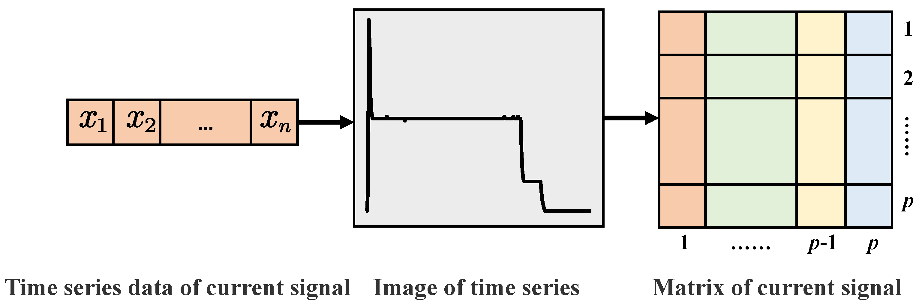
34]. Information on the action current curve was concentrated in the curved part, which could then be transformed into a binary image by converting the curve-sequence data. Each image was of size 32 × 32 . This processing method not only standardized the input format in the data preprocessing stage but also did not require complex signal-processing calculations or destroy the spatial structure of the current curve.

4.2. Experimental Setup

As mentioned previously, the proposed method was validated using actual turnout data from a subway. Comparative experiments were conducted to analyze the proposed method. All models were implemented on a computer with an NVIDIA RTX 3050 GPU and an Intel i5-12500H CPU. The proposed PL-MSMM hyperparameters included C, τ , and p. We conducted a detailed hyperparameter tuning process and determined the optimal combination of hyperparameter values by conducting experiments with different parameter combinations. Specifically, we chose C from { 1 × 10 3 , 2 × 10 3 , 5 × 10 3 , 1 × 10 2 , , 1 × 10 3 } and manually adjusted τ for each C, selecting p from { 0.1 , 0.2 , , 0.9 , 1 }
To thoroughly evaluate the classifier’s classification performance, we chose three evaluation metrics—that is, accuracy, precision, and F1-score. The F1-score can be calculated by precision and recall. Because the precision, recall, and F1-score are binary metrics, we adopted a macro-averaging approach to average the same measurements computed for each individual class. These evaluation metrics can be expressed as follows:
Accuracy = c = 1 k TP c T o t a l ,
Precision = 1 k c = 1 k TP c TP c + FP c ,
Recall = 1 k c = 1 k TP c TP c + FN c ,
F 1 - Score = 2 1 Recall + 1 Precision ,
where TP c , FP c , FN c , and TN c denote true positives, false positives, false negatives, and true negatives, respectively.

4.3. Comparison with Existing Methods

The proposed method was compared with existing fault diagnosis models to evaluate its performance. The compared models included the convolutional autoencoder (CAE) [35], CNN [36], and MSMM [29] models. Details of the methods and their parameter adjustments can be summarized as follows:
CAE: The input image size was 32 × 32 . The encoder contained two convolutional layers. The first and second convolutional layers had 20 kernels of size 3 × 3 and one kernel of size 3 × 3 , respectively. A pooling layer was added after each layer. The decoder included two deconvolutional layers with the same convolutional kernel size. The network used the Adam optimizer and rectified linear unit (ReLU) activation function, with an initial learning rate of 0.001 and a maximum iteration number of 100.
CNN: The input image size was 32 × 32 . The model structure included convolutional, batch normalization, ReLU activation function, max pooling, fully connected, and SoftMax layers. The convolutional layers had 20 kernels of dimensions 5 × 5 . Network training used a stochastic gradient descent with momentum (SGDM) optimizer. The initial learning rate was 0.001 and the number of iterations was 100.
MSMM: The training and testing datasets input to the model were two-dimensional images of size 32 × 32 . This model was applied to the fault diagnosis problem of turnouts based on current signals. The feature matrix obtained from the data preprocessing was used as the input to train the classifier. All the hyperparameters involved were selected through cross-validation.
The details of the hyperparameter settings and tune ranges in the models are listed in Table 2. The learning rate, batch size, and number of epochs are represented as r, b, and e, respectively. The MSMM parameters are C and τ .
The model was applied to the problem of current signal-based turnout fault diagnosis, and the image matrix features obtained from data preprocessing were used as inputs to train the classifier. To evaluate the performance of these methods, a ten-fold cross-validation method was adopted. Cross-validation is a widely used model evaluation method in machine learning. In k-fold cross-validation, the dataset is divided into k random subsets, with one subset chosen as the testing set and the remaining subsets used as the training set in each iteration [37]. This process helps mitigate the adverse effects caused by imbalanced data partitioning in a single split, leading to a more reliable and accurate assessment of the model’s performance. By averaging the results of multiple evaluations, cross-validation provides a more comprehensive and robust estimation of the model’s effectiveness [38]. The advantages of cross-validation are particularly evident in small-scale datasets, where the impact of imbalanced partitioning is more pronounced. For each class of samples, we randomly selected 500 to form the dataset. The accuracy, precision, and F1-score of the different methods were compared and analyzed using 10-fold cross-validation. The results are shown in Table 3 and Figure 6.
In Table 3, the average testing and training accuracy, precision, and F1-score of the four models are presented. The results show that the proposed PL-MSMM method outperforms the other methods in terms of accuracy, precision, and F1-score. The comparative results between matrix learning models (MSMM and PL-MSMM) and non-matrix learning models (CAE and CNN) indicate that the inclusion of structural information from 2D images significantly enhances diagnostic performance. Matrix learning models, which consider the structural information of the input data, have demonstrated superior results. 
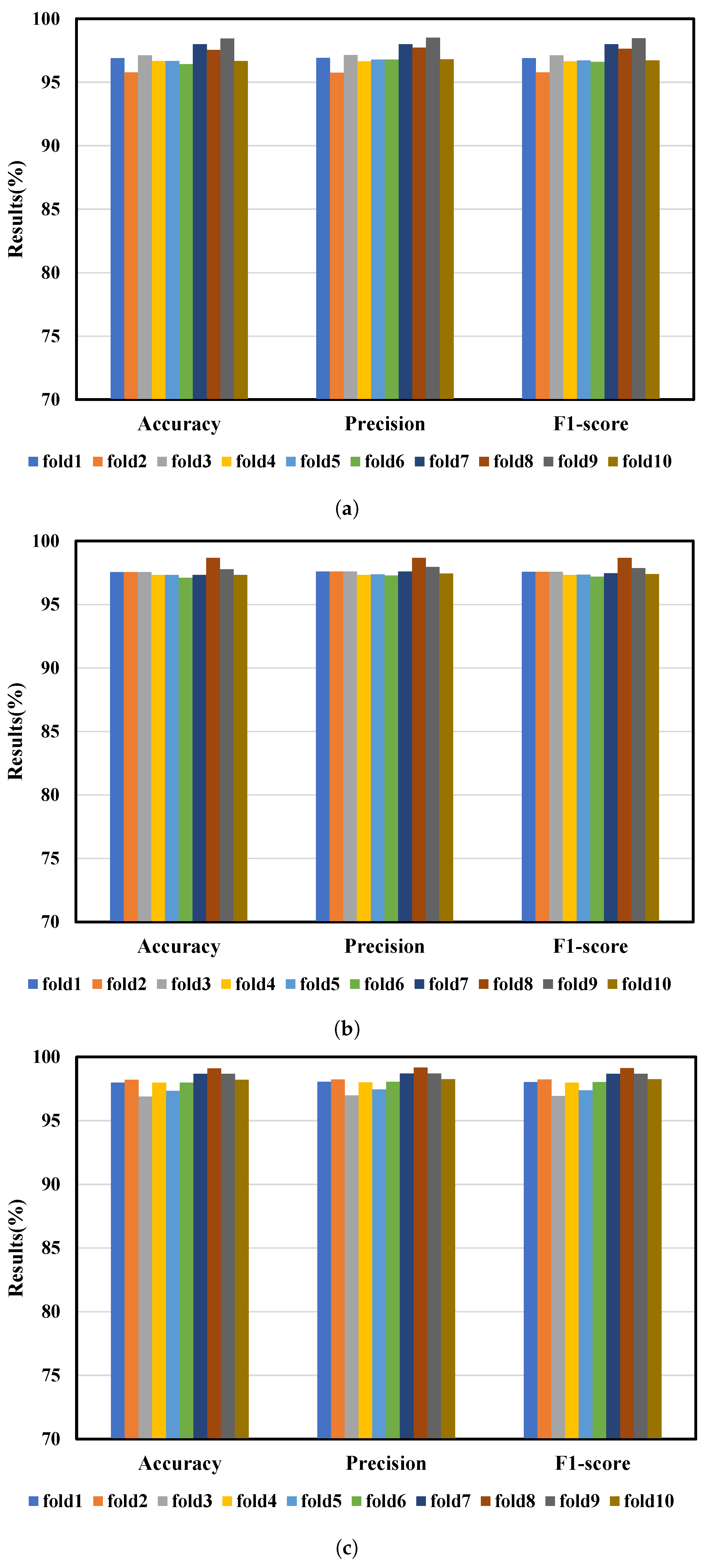
Figure 6a–d show the testing accuracy, precision, and F1-score when applying 10-fold cross-validation to the four models. It can be seen that the minimum accuracy of PL-MSMM is 98.22% and the maximum accuracy is 99.56%. The overall average classification accuracy can reach 98.67%. Among the 10-fold cross-validation, PL-MSMM achieves the highest accuracy. Its overall diagnostic performance is significantly superior to that of the other models under consideration. In summary, these experimental results show that the proposed PL-MSMM method performed excellently in turnout data fault diagnosis. This provides a feasible fault diagnosis method for practical applications and can achieve efficient fault diagnosis.
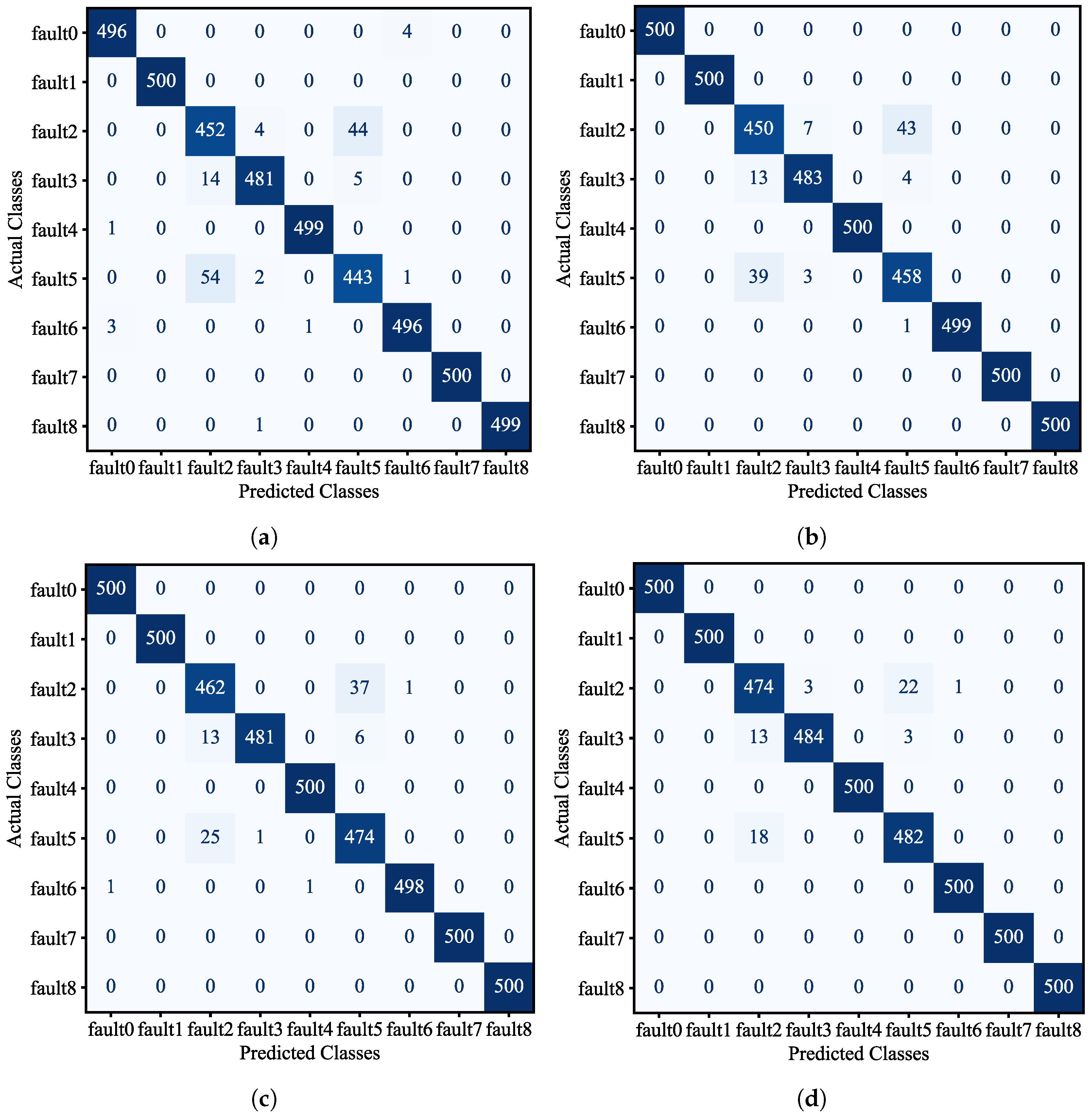
To enhance the illustration of the fault diagnosis results, Figure 7a–d display the confusion matrix generated by four different models. The confusion matrix provides a visual representation of the relationship between the model’s predicted results and the actual labels across various categories, presented in a matrix format. In the confusion matrix, each column represents the predicted categories, while each row corresponds to the true categories of the data. The elements on the main diagonal of the matrix indicate the number of correct classifications for each respective category.

4.4. Noise Sensitivity Analysis of PL-MSMM

To assess the robustness of the PL-MSMM algorithm, we added noise to the input image and compared it with the case without added noise. We chose the MSMM for comparison. For this experiment, we employed 10-fold cross-validation to evaluate the fault diagnosis accuracy of both methods. Table 4 presents the average testing and training accuracy, precision, and F1-score of the experimental methods. It should be noted that “Clean” means using the original input image without added noise and “SPN” means using the input image with salt and pepper noise added.
It is evident that the proposed algorithm outperforms the MSMM method, indicating its effective handling of noise in the input data while maintaining high classification accuracy and robustness. In contrast, the MSMM method performs poorly when noise is added, suggesting its difficulty in coping with noisy data, which leads to a degraded classification performance. The results show that the proposed algorithm exhibits a smaller accuracy difference of 0.99 compared to the MSMM method’s difference of 1.62 when noise is present. The proposed algorithm demonstrates relatively smaller fluctuations in results when affected by noise. Furthermore, when considering the relative percentage difference (RPD) as a metric, the RPD value for the PL-MSMM method, relative to the accuracy without noise, is 1.00%. In comparison, the RPD value for the MSMM method is 1.65%. This indicates that the percentage decrease in performance when handling noisy data is smaller when using the PL-MSMM method. Owing to the noise insensitivity of the pinball loss function, the PL-MSMM achieves better results than the MSMM on noise-contaminated datasets. This shows that the PLMSMM can handle noise-containing turnout fault datasets more effectively, with robustness and reliability.

4.5. Parameter Sensitivity Analysis of the Proposed PL-MSMM

Finally, a hyperparameter sensitivity experiment was conducted for the proposed PL-MSMM. The training dataset consisted of 20 randomly selected samples from each class, and the test dataset consisted of 20 randomly selected samples. Hyperparameter C was adjusted as follows: { 0.01 , 0.1 , 1 , 10 , 100 , 200 , 300 , 400 , 500 , 600 } . The accuracy of the PL-MSMM on the current dataset is shown in Table 5 and Figure 8.
The experimental results show that the performance of the PL-MSMM is sensitive to hyperparameter C. The choice of hyperparameters depends on the performance of the model in terms of the evaluation metrics. The influence parameter p on accuracy was also analyzed; the accuracy performance under different p values is shown in Table 6 and Figure 9.
The experimental results show that hyperparameter p has an impact on the model’s performance. Consequently, we need to choose an appropriate p value to obtain the best performance based on the specific application scenario and dataset.

5. Conclusions

The fault diagnosis of railway turnouts is critical for ensuring safe and reliable railway operations. This work developed an effective data-driven approach for diagnosing turnout faults using time-series monitoring data. An intelligent fault diagnosis method for railway turnouts with the support matrix machine was proposed. We have developed a data-driven intelligent method for diagnosing railway turnout faults, which considers the unique attributes of time series monitoring data. To address the noise sensitivity limitations inherent in the multiclass support matrix machine (MSMM), we introduced the pinball loss-based multiclass support matrix machine (PL-MSMM), which is adept at handling noisy industrial data. First, the proposed method employed the original one-dimensional time-series signal to generate a two-dimensional image through data preprocessing. Subsequently, the two-dimensional image matrix was the feature matrix. Next, the proposed PL-MSMM was built by the feature matrix to realize the turnout fault diagnosis. We conducted validation experiments on the proposed method using a current real-world turnout dataset. The effectiveness of the proposed method was verified via a comparative analysis. The proposed method is useful for fault diagnosis of railway turnouts. The diagnostic capabilities developed in this work can enable the condition-based maintenance of turnouts, reducing failures and downtime. By supporting predictive analytics on railway assets, this research promotes sustainable and reliable transportation infrastructure.
Although the proposed PL-MSMM approach has demonstrated proficiency in diagnosing railway turnout system failures, its reliance on extensive labeled data is a limitation, as such data are often scarce and demand considerable domain expertise for accurate annotation. Hence, the feasibility and expense of data labeling present a clear constraint. Future endeavors will explore semi-supervised or unsupervised learning strategies to diminish the reliance on labeled datasets, aiming to further enhance the efficiency and accuracy of fault diagnosis.

Author Contributions

Conceptualization, M.G. and Z.X.; methodology, M.G.; software, M.G.; validation, M.G.; formal analysis, M.G.; investigation, M.G. and M.M.; resources, Z.X.; writing—original draft preparation, M.G.; writing—review and editing, M.G.; supervision, Z.X.; project administration, M.M. All authors have read and agreed to the published version of the manuscript.

Funding

This research was funded by the National Key Research and Development Program of China under Grant 2022YFB4300504-4 and Special Fund Project supported by Shanghai Municipal Commission of Economy and Information Technology under Grant 202201034.

Institutional Review Board Statement

Not applicable.

Informed Consent Statement

Not applicable.

Data Availability Statement

The data presented in this study are available on request from the corresponding author. The data are not publicly available due to privacy.

Acknowledgments

The authors would like to thank the all-round rail transit control system integrator (CASCO) for providing research data and domain knowledge support.

Conflicts of Interest

The authors declare no conflict of interest.

Abbreviations

The following abbreviations are used in this manuscript:
CAEConvolutional autoencoder
CNNConvolutional neural network
MSMMMulticlass support matrix machine
PHMPrognostics and health management
PL-MSMMPinball loss-based multiclass support matrix machine
SMMSupport matrix machine

References

  1. Xie, S.; Tan, H.; Yang, C.; Yan, H. A Review of Fault Diagnosis Methods for Key Systems of the High-Speed Train. Appl. Sci. 2023, 13, 4790. [Google Scholar] [CrossRef]
  2. Chen, C.; Li, X.; Huang, K.; Xu, Z.; Mei, M. A Convolutional Autoencoder Based Fault Detection Method for Metro Railway Turnout. CMES-Comput. Model. Eng. Sci. 2023, 136, 471–485. [Google Scholar] [CrossRef]
  3. Ji, W.; Cheng, C.; Xie, G.; Zhu, L.; Wang, Y.; Pan, L.; Hei, X. An intelligent fault diagnosis method based on curve segmentation and SVM for rail transit turnout. J. Intell. Fuzzy Syst. 2021, 41, 4275–4285. [Google Scholar] [CrossRef]
  4. Zhang, R.; Li, Z. Multi-fault diagnosis scheme based on robust nonlinear observer with application to rolling mill main drive system. Trans. Inst. Meas. Control 2023, 45, 1245–1257. [Google Scholar] [CrossRef]
  5. Hu, X.; Cao, Y.; Tang, T.; Sun, Y. Data-driven technology of fault diagnosis in railway point machines: Review and challenges. Transp. Saf. Environ. 2022, 4, tdac036. [Google Scholar] [CrossRef]
  6. Wang, Z.; Wang, N.; Zhang, H.; Jia, L.; Qin, Y.; Zuo, Y.; Zhang, Y.; Dong, H. Segmentalized mRMR features and cost-sensitive ELM with fixed inputs for fault diagnosis of high-speed railway turnouts. IEEE Trans. Intell. Transp. Syst. 2023, 24, 4975–4987. [Google Scholar] [CrossRef]
  7. Hamadache, M.; Dutta, S.; Olaby, O.; Ambur, R.; Stewart, E.; Dixon, R. On the fault detection and diagnosis of railway switch and crossing systems: An overview. Appl. Sci. 2019, 9, 5129. [Google Scholar] [CrossRef]
  8. Ji, W.; Zuo, Y.; Fei, R.; Xie, G.; Zhang, J.; Hei, X. An Adaptive Fault Diagnosis Model for Railway Single and Double Action Turnout. IEEE Trans. Intell. Transp. Syst. 2022, 24, 1314–1324. [Google Scholar] [CrossRef]
  9. Zhang, K.; Huang, W.; Hou, X.; Xu, J.; Su, R.; Xu, H. A fault diagnosis and visualization method for high-speed train based on edge and cloud collaboration. Appl. Sci. 2021, 11, 1251. [Google Scholar] [CrossRef]
  10. Lao, Z.; He, D.; Wei, Z.; Shang, H.; Jin, Z.; Miao, J.; Ren, C. Intelligent fault diagnosis for rail transit switch machine based on adaptive feature selection and improved LightGBM. Eng. Fail. Anal. 2023, 148, 107219. [Google Scholar] [CrossRef]
  11. Chen, C.; Shao, H.; Xu, Z.; Huang, K.; Chen, Q.; Mei, M. A Fault Detection Method for Railway Turnout with Convex Hull-based One-Class Tensor Machine. In Proceedings of the 2023 IEEE International Instrumentation and Measurement Technology Conference (I2MTC), Kuala Lumpur, Malaysia, 22–25 May 2023; IEEE: Piscataway, NJ, USA, 2023; pp. 1–6. [Google Scholar]
  12. Han, T.; Jiang, D.; Zhao, Q.; Wang, L.; Yin, K. Comparison of random forest, artificial neural networks and support vector machine for intelligent diagnosis of rotating machinery. Trans. Inst. Meas. Control 2018, 40, 2681–2693. [Google Scholar] [CrossRef]
  13. Sun, Y.; Cao, Y.; Xie, G.; Wen, T. Sound based fault diagnosis for RPMs based on multi-scale fractional permutation entropy and two-scale algorithm. IEEE Trans. Veh. Technol. 2021, 70, 11184–11192. [Google Scholar] [CrossRef]
  14. Chen, Q.; Nicholson, G.; Roberts, C.; Ye, J.; Zhao, Y. Improved fault diagnosis of railway switch system using energy-based thresholding wavelets (EBTW) and neural networks. IEEE Trans. Instrum. Meas. 2020, 70, 1–12. [Google Scholar] [CrossRef]
  15. Li, W.; Li, G. Railway’s Turnout Fault Diagnosis Based on Power Curve Similarity. In Proceedings of the 2019 International Conference on Communications, Information System and Computer Engineering (CISCE), Haikou, China, 5–7 July 2019; IEEE: Piscataway, NJ, USA, 2019; pp. 112–115. [Google Scholar]
  16. Zheng, Y.; Bai, D.; Yan, W. Research on turnout health state assessment and fault detection method based on similarity. J. Railw. Sci. Eng. 2021, 18, 877–884. [Google Scholar]
  17. Huang, S.; Yang, X.; Wang, L.; Chen, W.; Zhang, F.; Dong, D. Two-stage turnout fault diagnosis based on similarity function and fuzzy c-means. Adv. Mech. Eng. 2018, 10, 1687814018811402. [Google Scholar] [CrossRef]
  18. Xiao, Y.; Shao, H.; Feng, M.; Han, T.; Wan, J.; Liu, B. Towards trustworthy rotating machinery fault diagnosis via attention uncertainty in Transformer. J. Manuf. Syst. 2023, 70, 186–201. [Google Scholar] [CrossRef]
  19. Lin, J.; Shao, H.; Zhou, X.; Cai, B.; Liu, B. Generalized MAML for few-shot cross-domain fault diagnosis of bearing driven by heterogeneous signals. Expert Syst. Appl. 2023, 230, 120696. [Google Scholar] [CrossRef]
  20. Yan, S.; Zhong, X.; Shao, H.; Ming, Y.; Liu, C.; Liu, B. Digital twin-assisted imbalanced fault diagnosis framework using subdomain adaptive mechanism and margin-aware regularization. Reliab. Eng. Syst. Saf. 2023, 239, 109522. [Google Scholar] [CrossRef]
  21. Guo, Z.; Ye, H.; Jiang, M.; Sun, X. An enhanced fault detection method for railway turnouts incorporating prior faulty information. In Proceedings of the 2020 IEEE 23rd International Conference on Intelligent Transportation Systems (ITSC), Rhodes, Greece, 20–23 September 2020; IEEE: Piscataway, NJ, USA, 2020; pp. 1–6. [Google Scholar]
  22. Li, M.; Hei, X.; Ji, W.; Zhu, L.; Wang, Y.; Qiu, Y. A Fault-Diagnosis Method for Railway Turnout Systems Based on Improved Autoencoder and Data Augmentation. Sensors 2022, 22, 9438. [Google Scholar] [CrossRef]
  23. Lao, Z.; He, D.; Jin, Z.; Liu, C.; Shang, H.; He, Y. Few-shot fault diagnosis of turnout switch machine based on semi-supervised weighted prototypical network. Knowl.-Based Syst. 2023, 274, 110634. [Google Scholar] [CrossRef]
  24. Yan, S.; Shao, H.; Min, Z.; Peng, J.; Cai, B.; Liu, B. FGDAE: A new machinery anomaly detection method towards complex operating conditions. Reliab. Eng. Syst. Saf. 2023, 236, 109319. [Google Scholar] [CrossRef]
  25. Chen, C.; Mei, M.; Shao, H.; Liang, P. A support tensor machine-based fault diagnosis method for railway turnout. In Proceedings of the 2023 IEEE International Conference on Prognostics and Health Management (ICPHM), Montreal, QC, Canada, 5–7 June 2023; IEEE: Piscataway, NJ, USA, 2023; pp. 274–281. [Google Scholar]
  26. Li, X.; Cheng, J.; Shao, H.; Liu, K.; Cai, B. A fusion CWSMM-based framework for rotating machinery fault diagnosis under strong interference and imbalanced case. IEEE Trans. Ind. Inform. 2021, 18, 5180–5189. [Google Scholar] [CrossRef]
  27. Luo, L.; Xie, Y.; Zhang, Z.; Li, W.J. Support matrix machines. In Proceedings of the International Conference on Machine Learning. PMLR, San Diego, CA, USA, 9–12 May 2015; pp. 938–947. [Google Scholar]
  28. Li, X.; Shao, H.; Lu, S.; Xiang, J.; Cai, B. Highly efficient fault diagnosis of rotating machinery under time-varying speeds using LSISMM and small infrared thermal images. IEEE Trans. Syst. Man Cybern. Syst. 2022, 52, 7328–7340. [Google Scholar] [CrossRef]
  29. Zheng, Q.; Zhu, F.; Qin, J.; Heng, P.A. Multiclass support matrix machine for single trial EEG classification. Neurocomputing 2018, 275, 869–880. [Google Scholar] [CrossRef]
  30. Feng, R.; Xu, Y. Support matrix machine with pinball loss for classification. Neural Comput. Appl. 2022, 34, 18643–18661. [Google Scholar] [CrossRef]
  31. Boyd, S.; Parikh, N.; Chu, E.; Peleato, B.; Eckstein, J. Distributed optimization and statistical learning via the alternating direction method of multipliers. Found. Trends Mach. Learn. 2011, 3, 1–122. [Google Scholar] [CrossRef]
  32. Zheng, Q.; Zhu, F.; Qin, J.; Chen, B.; Heng, P.A. Sparse support matrix machine. Pattern Recognit. 2018, 76, 715–726. [Google Scholar] [CrossRef]
  33. Zhang, P.; Zhang, G.; Dong, W.; Sun, X.; Ji, X. Fault diagnosis of high-speed railway turnout based on convolutional neural network. In Proceedings of the 2018 24th International Conference on Automation and Computing (ICAC), Newcastle upon Tyne, UK, 6–7 September 2018; IEEE: Piscataway, NJ, USA, 2018; pp. 1–6. [Google Scholar]
  34. Chawla, N.V.; Bowyer, K.W.; Hall, L.O.; Kegelmeyer, W.P. SMOTE: Synthetic minority over-sampling technique. J. Artif. Intell. Res. 2002, 16, 321–357. [Google Scholar] [CrossRef]
  35. Yang, D.; Sun, K. A CAE-based deep learning methodology for rotating machinery fault diagnosis. In Proceedings of the 2021 7th International Conference on Control, Automation and Robotics (ICCAR), Singapore, 23–26 April 2021; IEEE: Piscataway, NJ, USA, 2021; pp. 393–396. [Google Scholar]
  36. Gnanamalar, A.J.; Bhavani, R.; Arulini, A.S.; Veerraju, M.S. CNN–SVM Based Fault Detection, Classification and Location of Multi-terminal VSC–HVDC System. J. Electr. Eng. Technol. 2023, 18, 3335–3347. [Google Scholar] [CrossRef]
  37. Liu, C.; Wang, G.; Xie, Q.; Zhang, Y. Vibration sensor-based bearing fault diagnosis using ellipsoid-ARTMAP and differential evolution algorithms. Sensors 2014, 14, 10598–10618. [Google Scholar] [CrossRef]
  38. Suthar, V.; Vakharia, V.; Patel, V.K.; Shah, M. Detection of compound faults in ball bearings using multiscale-SinGAN, heat transfer search optimization, and extreme learning machine. Machines 2022, 11, 29. [Google Scholar] [CrossRef]
Figure 1. Turnout structural schematic.
Applsci 13 12375 g001
Figure 2. Framework of the proposed turnout diagnosis method.
Applsci 13 12375 g002
Figure 3. Process of converting time series data into 2D image.
Applsci 13 12375 g003
Figure 4. A-phase current curve.
Applsci 13 12375 g004
Figure 5. ZDJ9 turnout fault 0−8 current curves.
Applsci 13 12375 g005
Figure 6. The accuracy under each fold: (a) CAE, (b) CNN, (c) MSMM, and (d) PL-MSMM.
Applsci 13 12375 g006aApplsci 13 12375 g006b
Figure 7. Confusion matrix from 10-fold cross-validation: (a) CAE, (b) CNN, (c) MSMM, and (d) PL-MSMM.
Applsci 13 12375 g007
Figure 8. Performance graph for the model according to parameter C.
Applsci 13 12375 g008
Figure 9. Performance graph for the model according to parameter p.
Applsci 13 12375 g009
Table 1. Analysis of different types of current curves of ZDJ9 turnouts.
Fault LabelsFault PhenomenonFault Cause
fault 0Normal stateNormal
fault 1The current is zeroAction circuit fault
fault 2The current is constantMechanical resistance
fault 3The current suddenly becomes zeroThe point machine is not unlocked or in good contact
fault 4Small step current interruptionThe contact of point machine is abnormal
fault 5The current increasesThe point machine friction increases and internal jamming
fault 6No small step current during actionThe indicate circuit is abnormal
fault 7Spikes in the currentPoor contact of the switch circuit controller
fault 8The current is large, the curve only maintains 0∼1 sPhase failure of the starting circuit
Table 2. Hyperparameter setting and tune range of the models used in the comparison.
ModelHyperparametersTraining Range
CAE { r , b , e } { [ 0.0001 , 1 ] , [ 32 , 256 ] , [ 10 , 1000 ] }
CNN { r , b , e } { [ 0.0001 , 1 ] , [ 32 , 256 ] , [ 10 , 500 ] }
MSMM { C , τ } { [ 0.001 , 1000 ] , [ 0 , 10 ] }
Table 3. The average testing and training accuracy, precision, and F1-score for different methods.
TestingTraining
MethodAccyracy (%)Precision (%)F1-Score (%)Accuracy (%)Precision (%)F1-Score (%)
CAE97.0297.1197.0797.8797.9697.92
CNN97.5697.6597.6097.9798.0698.01
MSMM98.1198.1798.1498.0798.1298.09
PL-MSMM98.6798.7098.6898.7498.7798.76
Table 4. Performance comparison of PL-MSMM and MSMM with or without noise using 10-fold cross-validation.
TestingTraining
MethodNoiseAccyracy (%)Precision (%)F1-Score (%)Accuracy (%)Precision (%)F1-Score (%)
MSMMClean98.1198.1798.1498.0798.1298.09
SPN96.4996.6596.5798.4598.598.48
PL-MSMMClean98.6798.7098.6898.7498.7798.76
SPN97.6797.7597.7198.1998.2398.21
Table 5. PL-MSMM performance with different parameter C values.
C0.010.1110100200300400500600
Accuracy (%)50.0050.0041.6778.8992.2291.6793.3391.6794.4492.22
Table 6. PL-MSMM performance with different parameter p values.
p00.10.20.30.40.50.60.70.80.9
Accuracy (%)92.7892.2292.7892.7893.3389.4494.4493.3393.3390.56
Disclaimer/Publisher’s Note: The statements, opinions and data contained in all publications are solely those of the individual author(s) and contributor(s) and not of MDPI and/or the editor(s). MDPI and/or the editor(s) disclaim responsibility for any injury to people or property resulting from any ideas, methods, instructions or products referred to in the content.

