Research on Driving Style Recognition of Autonomous Vehicles Based on ACO-BP

Abstract

To enhance the lane-changing safety of autonomous vehicles, it is crucial to accurately identify the driving styles of human drivers in scenarios involving the coexistence of autonomous and human-driven vehicles, aiming to avoid encountering vehicles exhibiting hazardous driving patterns. In this study, based on the real traffic flow data from the Next Generation Simulation (NGSIM) dataset in the United States, 301 lane-changing vehicles that meet the criteria are selected. Six evaluation parameters are chosen, and principal component analysis (PCA) is employed for dimensionality reduction in the data. The K-means algorithm is then utilized to cluster the driving styles, classifying them into three categories. Finally, ant colony optimization (ACO) of a backpropagation (BP) neural network model was constructed, utilizing the dimensionality reduction results as inputs and the clustering results as outputs for the purpose of driving style recognition. Simulation experiments are conducted using MATLAB Version 9.10 (R2021a) for comparative analysis. The results indicate that the constructed ACO-BP model achieved an overall recognition accuracy of 96.7%, significantly higher than the recognition accuracies of the BP, artificial neural network (ANN), and gradient boosting machine (GBM) models. The ACO-BP model also exhibited the fastest recognition speed among the four models. Moreover, the ACO-BP model shows varied improvements in recognition accuracy for each of the three driving styles, with an increase of 13.7%, 4.4%, and 4.3%, respectively, compared to the BP model. The simulation results validate the high accuracy, real-time capability, and classification effectiveness of this model in driving style recognition, providing new insights for this field.

1. Introduction

Autonomous driving is an advanced automotive technology that utilizes onboard sensors, computer vision, and machine learning to enable vehicles to autonomously perceive, analyze, and respond to road environments, achieving full or partial driverless operation [1]. Through autonomous driving technology, vehicles can automatically control their movements, comply with traffic rules, avoid obstacles, and make reasonable driving decisions based on the actual road conditions [2]. The development of this technology aims to enhance road safety, reduce traffic accidents, improve traffic efficiency, and provide passengers with a more convenient and comfortable travel experience. Although autonomous driving faces challenges in various traffic environments, with continuous technological advancements and practical implementations, it will become a significant direction for future developments in the transportation field.

With the continuous advancement of autonomous driving technology and the increasing number of road tests and commercial operations of autonomous vehicles, mixed traffic flow composed of autonomous and human-driven vehicles is expected to be a future development trend. As a result, the market share of autonomous vehicles in the automotive industry is also projected to increase [3]. Currently, research on autonomous driving technology is extensive, covering aspects such as trajectory prediction [4], comfort [5], and urban road traffic efficiency [6]. In the human–vehicle–road traffic system, drivers, as the main participants, have a significant impact on road traffic safety [7]. Different driving styles have varying effects on vehicle lane-changing safety [8]. For instance, drivers with aggressive driving styles have higher demands for speed and time benefits, resulting in reduced safety levels and a higher accident rate. Therefore, researching driver style recognition technology is of great significance as it can enhance the safety of lane changing for autonomous vehicles to a certain extent.

The main objective of current research is to improve the accuracy and real-time capability of driver style recognition. At present, one widely applied technique in various fields, such as architecture and mathematical analysis, is the ACO-BP hybrid model, known for its accurate prediction performance and fast prediction speed [9,10,11]. Therefore, this study aims to investigate the practical application of the ACO-BP hybrid model in the direction of autonomous driving style recognition. In this paper, real vehicle driving data from the NGSIM dataset is utilized, and vehicle historical trajectory data that meet the requirements are selected to avoid the risk of overfitting caused by small-sample data. By using principal component analysis for dimensionality reduction and employing K-means clustering analysis to categorize driving styles, a driving style recognition model based on ant colony optimization of a BP neural network is established. This model enables the identification and prediction of driving styles, thus enabling the timely avoidance of hazardous driving styles during lane-changing maneuvers.

The remaining organization of this paper is as follows: Section 2 provides an overview of the research status of automatic driving style recognition. Section 3 presents the methodology and data, including a description of the ACO-BP model, the extraction and processing of vehicle data, feature extraction, and driving style clustering. Section 4 mainly presents the recognition results of the established ACO-BP driving style recognition model. Section 5 compares the ACO-BP model with other previously applied automatic driving style recognition models (ANN and GBM), further discussing the reliability of the ACO-BP model. Finally, this paper summarizes the research and provides prospects for future optimization research directions.

2. Literature Review

In the continuous advancement of autonomous driving technology, many scholars have come to consider that lane-changing accidents account for a considerable proportion of traffic accidents. Aggressive driving styles often involve frequent lane changes, smaller following distances, and more drastic acceleration changes, which highlights the importance of improving the accuracy of lane-changing recognition in autonomous driving to reduce safety hazards and mitigate such risky driving styles. Therefore, in the current research on the safety of autonomous driving lane changing, much attention has been focused on the field of automatic driving style recognition technology.

One of the most widely applied technologies is traditional machine learning algorithms. Traditional machine learning algorithms mainly include support vector machines (SVMs), decision trees, and random forests. Kumar et al. compared the recognition effects of models using SVMs, adaptive boosting (AdaBoost), and random forest algorithms by extracting data from internal sensors in the engine through the On-Board Diagnostics II (OBD-II) protocol, achieving good recognition accuracy [12]. Peng et al. proposed a driving style recognition model based on the Classification and Regression Tree (CART) decision-making method by clustering indicators such as following distance, time gap, and accelerator pedal opening, and their experimental results demonstrated its good recognition accuracy [13]. Zhao et al. collected natural driving trajectory data in freeway diverging areas using unmanned aerial vehicles and applied K-means++ to cluster the driving styles in lane-changing sections. They achieved an accuracy of 93% using a random forest model for driving style identification and prediction [14].

With the advancement of onboard sensor technology, vehicles are capable of collecting a large amount of data for deep learning training. Simultaneously, due to improvements in computational power, algorithms, and other factors, deep learning has gained popularity in the field of automated driving style recognition [15]. Milardo et al. proposed a deep neural network architecture using unsupervised feature extraction, feature selection algorithms, and automated machine learning (AutoML) techniques. They validated the model using real road driving data in random environments, achieving a driving style recognition accuracy of 95% [16]. Bejani et al. developed an adaptive regularization convolutional neural network (CNN) to avoid overfitting when performing driving style recognition on smartphones [17]. Xu et al. introduced a driving style recognition system with a combination of a fully convolutional network (FCN) and a squeeze-and-excitation (SE) block. They used psychophysical and behavioral data for driving style recognition and validation [18]. Liang et al. proposed a comprehensive driving style recognition model based on driving cycle identification. They constructed a driving style cycle and recognition model using an artificial neural network (ANN), enabling more comprehensive and accurate long-term driving style recognition [19].

Nowadays, with the increase in vehicle ownership and the complexity of urban road networks, higher demands are being placed on autonomous driving technology. In response, hybrid models combining traditional machine learning algorithms with deep learning have emerged. Zhang et al. utilized the Next Generation Simulation (NGSIM) traffic flow dataset and proposed the Adaptive Multivariate Continuous Gaussian Mixture Hidden Markov Model (AMCGM-HMM) for dynamic driving intention recognition of surrounding vehicles, thereby enhancing vehicle driving safety [20]. Cai et al. addressed incomplete traffic data and proposed a Convolutional Neural Network—Long Short-Term Memory (CNN-LSTM)-based driving style recognition model, which improved recognition accuracy and generalization capabilities [21]. Additionally, Kim et al. proposed a Deep Convolutional Long Short-Term Memory (DCLSTM)-based driving style recognition model to improve the safety of autonomous vehicle trajectories and predict future trajectories [22].

Despite extensive research on automatic driving style recognition, there are still some limitations. In general:

• The advantages of traditional machine learning models include easy interpretability, high computational efficiency, and good classification performance on linearly separable problems such as SVMs. However, their disadvantages include poor performance on high-dimensional complex datasets and inadequate classification performance on nonlinearly separable problems.
• The advantages of deep learning lie in its ability to handle high-dimensional, nonlinear, and complex problems, and it performs well on different types of data, such as images, speech, and text. However, its disadvantages include the tendency to overfit, the requirement for large datasets to achieve good performance, and the need for substantial computational resources for network design and parameter tuning.
• Hybrid models combine the strengths of both traditional machine learning and deep learning, offering good generalization to different datasets and tasks, strong interpretability, computational efficiency, and expressive power. However, their disadvantages lie in their increased complexity, which adds to the development difficulty, and their increased demand for computational resources in terms of model fusion and parameter optimization.

Therefore, in practical research on automatic driving style recognition, the choice of suitable algorithms should be made by considering specific problems and dataset characteristics. Factors to be considered include the size and complexity of the dataset, computational requirements, real-time constraints, accuracy, and robustness of the algorithm.

3. Methodology

3.1. Introduction to the ACO-BP Model

3.1.1. BP Neural Network

The BP neural network is a common type of artificial neural network that can be applied to problems such as recognition, classification, and prediction [23]. The BP neural network exhibits several key benefits:

• Strong nonlinear fitting ability, capable of handling complex nonlinear problems.
• Good adaptive ability, able to automatically adjust the network parameters according to the changes in the input data, to improve the robustness of the model and generalization ability.
• It has good fault tolerance and can maintain good performance even if some neurons or connections in the network fail.
• Good interpretability, with the network structure and parameters capable of adjusting to understand the workings of the network and the decision-making process.

The transfer function for the input and hidden layers of the BP neural network is set as $tansig$, while the transfer function for the output layer is defined as $purelin$. The training function selected for the network is $trainlm$. The hidden layer can have more than one layer, but due to the requirements of the accuracy of the recognition of the driving style, this paper’s implicit layer selected a layer with the specific topology shown in Figure 1.

Training Steps for the BP Neural Network:

Step 1: Determine the basic structure of the BP neural network, including the number of nodes in the input layer (n), the number of nodes in the hidden layer (r), and the number of nodes in the output layer (l). Set the initial parameter values.

Step 2: Calculate the outputs of the hidden layer, as shown in Equation (1):

$$H_j=f({\displaystyle \sum _{i=1}^n{w}_{ij}{x}_i-a_j}),i=1,2,\cdots ,r$$

(1)

In Equation (1), $w_{ij}$ is the connection weight between the input layer and the hidden layer, $x_i$ represents the input vector, $a_j$ is the threshold of the hidden layer, and $tansig$ is the transfer function, as shown in Equation (2):

$$y=\frac{2}{1-e^{-2x}}-1$$

(2)

Step 3: Calculate the actual output of the output layer, as shown in Equation (3):

$$O_k={\displaystyle \sum _{j=1}^r{H}_j{w}_{jk}-b_k}$$

(3)

Step 4: Calculate the error $e_k$ between the network output and the true value, as shown in Equation (4):

$$e_k=O_k-Y_k$$

(4)

In Equation (4), $O_k$ represents the predicted value and $Y_k$ represents the true value.

Step 5: Update the weights and thresholds, as follows:

$$w_{ij}=w_{ij}+\eta H_j(1-H_j)x_i{\displaystyle \sum _{k=1}^m{w}_{ij}{e}_k,i=1,2,\cdots ,n;j=1,2,\cdots ,r}$$

(5)

$$w_{jk}=w_{jk}+\eta H_j{e}_k,j=1,2,\cdots ,r;k=1,2,\cdots ,m$$

(6)

$$a_j=a_j+\eta H_j(1-H_j){\displaystyle \sum _{k=1}^m{w}_{jk}{e}_k,j=1,2,\cdots ,r}$$

(7)

$$b_k=b_k+e_k,k=1,2,\cdots ,m$$

(8)

3.1.2. Ant Colony Algorithm

The ant colony algorithm is a heuristic algorithm developed by simulating ants’ behavior in searching for food. It finds the optimal solution by searching and optimizing the problem space. In the ant colony algorithm, ants search the problem space by releasing pheromones and guide the choices of other ants based on the change in pheromone concentration. The commonly used formula is as follows:

Calculate the probability $p_{ij}^k\left(t\right)$ that ant $k$ is at position $i$ going to position $j$ at time $t$ [24] with the following equation:

$$p_{ij}^k\left(t\right)=\left\{\begin{array}{c}\frac{{\left[{\tau }_{ij}\left(t\right)\right]}^{\alpha }{\left[{\eta }_{ij}\left(t\right)\right]}^{\beta }}{{{\displaystyle \sum }}_{s\in allowe{d}_k}{\left[{\tau }_{is}\left(t\right)\right]}^{\alpha }{\left[{\eta }_{is}\left(t\right)\right]}^{\beta }},j\in allowe{d}_k\\ 0,otherwise\end{array}\right.$$

(9)

In Equation (3), ${\tau }_{ij}$ is the pheromone; ${\eta }_{ij}\left(t\right)=\raisebox{1ex}{$1$}\!\left/ \!\raisebox{-1ex}{$d_{ij}$}\right.$ is the heuristic function, which indicates the expected degree of transferring ants from position $i$ to position $j$; and $allowe{d}_k\left(k=1,2,\cdots ,m\right)$ is the set of positions to be visited by the ant $k$. $\alpha$ represents the pheromone importance factor, and as its value increases, the significance of pheromone concentration in the transfer process also increases. $\beta$ represents the significance coefficient of the heuristic function, whereby a higher value signifies a greater influence of the heuristic function on the transfer process. In other words, as $\beta$ increases, the likelihood of ants transferring to locations with shorter distances also increases.

Once every ant in the system finishes a cycle, it becomes necessary to dynamically update the pheromone concentration on the path connecting each location in real-time [25], and the expression of the update equation is shown below:

$$\left\{\begin{array}{c}{\tau }_{ij}\left(t+1\right)=\left(1-\rho \right)\times {\tau }_{ij}\left(t\right)+\Delta {\tau }_{ij},0<\rho <1\\ \Delta {\tau }_{ij}={{\displaystyle \sum }}_{k=1}^n\Delta {\tau }_{ij}^k\end{array}\right.$$

(10)

In Equation (4), $\Delta {\tau }_{ij}^k$ is the amount of information left by the ant k on the path between position $i$ and position $j$ in this cycle, and $\Delta {\tau }_{ij}$ is the sum of pheromone concentration released by all ants on the path connecting position $i$ and $j$.

3.1.3. Utilizing the Ant Colony Algorithm for BP Neural Network Optimization

The basic idea of the optimization is to extract the elements of the weight matrix and threshold vector to form the path coordinates of the ant population. These elements collectively form the path coordinates of the ant population, constituting the fundamental concept underlying this approach. Because the shorter the path for ants to reach the food source, the higher the pheromone content on the path, the ants’ fitness value is determined by considering the mean square error. The shortest path determined by the final ant population is used as the optimal initial weights and threshold parameters, which are then assigned to the BP neural network, trained, and tested. To validate the rationality of the ACO-BP model, a comparison was conducted between its results and those obtained from the BP neural network. Figure 2 depicts the optimization process.

ACO-BP algorithm-specific steps:

Step 1: Read the data, initialize the structure of the BP neural network and the parameters of the ant colony optimization algorithm, and set the parameter set $I_{Pi}$.

Step 2: Place each ant on the initial starting point, where the number of ants is denoted as m and the number of paths chosen by ants is denoted as n. The ant k can randomly choose its element j according to the following probability:

$$P({\tau }_j^k(I_{Pi}))=\frac{{\tau }_j(I_{Pi})}{{\displaystyle \sum _{j=1}^n{\tau }_j(I_{Pi})}}$$

(11)

Step 3: Train the model, record the optimal solution, and update the pheromone $\tau$ in the set $I_{Pi}$. The pheromones on the paths from the initial position to the destination for each ant need to be adjusted according to the following equations:

$${\tau }_j(I_{Pi})(t+h)=\rho {\tau }_j(I_{Pi})(t)+\Delta {\tau }_j(I_{Pi})$$

(12)

$$\Delta {\tau }_j(I_{Pi})={\displaystyle \sum _{k=1}^m\Delta {\tau }_j^k(I_{Pi})}$$

(13)

In Equations (12) and (13), $\Delta {\tau }_j^k(I_{Pi})$ represents the amount of pheromone that ant k deposits on element j in one iteration, as shown in the equation:

$$\Delta {\tau }_j^k(I_{Pi})=\left\{\begin{array}{l}Q/e_k,thei-thantselectselement{P}_j(I_{Pi})\\ 0,other\end{array}\right.$$

(14)

In Equation (14), $Q$ is the fixed value of the pheromone, and $e_k$ is the output error of the neural network corresponding to ant k.

Step 4: Repeat steps 2 and 3 until the maximum number of iterations is reached, then proceed to step 5.

Step 5: Extract the coordinates of the best ant position after optimization and assign them to the BP neural network to obtain the optimal initial weight matrix and threshold vector.

Step 6: Train and test the optimized BP neural model and compare the recognition performance of the BP neural network before and after optimization.

Although ant colony optimization (ACO) sometimes falls into local optima, making it difficult to find the globally optimal configuration of neural networks, in ACO-BP, the ACO algorithm updates ant positions in each iteration based on certain rules (such as pheromone concentration and heuristic information) to explore new potential solutions. Additionally, ACO employs pheromone evaporation mechanisms and state transition rules to prevent premature convergence to local optima. In this process, the ACO algorithm not only retains the current best solution found (global optimum) but also stores the best solution found by each ant (local optimum). These local optima are reconsidered in subsequent iterations, thereby enhancing the algorithm’s ability to escape local optima. Moreover, when ACO is used for training BP neural networks, after each iteration, the gradient descent method can assist the ACO algorithm in achieving local optimization.

3.2. Data Processing and Screening

3.2.1. Data Source

In this paper, the NGSIM (Next Generation Simulation) traffic dataset is used for the study as a source of simulation data [26]. Its main advantages are as follows:

(1)

The NGSIM dataset contains a large amount of traffic flow data, including different time periods and different road types and traffic conditions, which can provide comprehensive traffic behavior information.

(2)

The NGSIM dataset has a high degree of authenticity, accuracy, and more comprehensive data [27], which can provide a reliable research basis and is widely used in microscopic traffic simulation modeling.

(3)

The NGSIM dataset has a sampling accuracy of 0.1 s, which provides high temporal and spatial resolution traffic data, and continuously records traveling data such as vehicle category, speed, acceleration, headway, and headway hourly distance, which accurately describes the traveling state of vehicles.

In this paper, we selected the US-101 freeway collection section data from the NGSIM dataset to screen the suitable lane-changing vehicles, and the specific applicable conditions are as follows:

(1)

Vehicle driving road conditions are freeways.

(2)

Only small cars are used as research objects.

(3)

Screening for free lane changing and single lane changing vehicles: only lane changing vehicles in lanes 1 to 5 are considered due to the impact of converging traffic on ramps 7 and 8.

(4)

Screening of vehicles with a distance of 5 m to 60 m between the following vehicles.

(5)

The process of lane-changing for a vehicle encompasses the leading vehicle in the current lane, the leading vehicle in the intended lane, and the trailing vehicle in the intended lane.

Taking ID64 vehicles as an example, the screening data is shown in

Table 1. Partial screening data for ID64 vehicles.

Vehicle ID	Frame Rate	Vehicle Speed (m·s−1)	Acc (m·s−2)	Following Distance (m)	Following Distance (s)
64	163	10.912	0	23.35	1.56
	…	…	…	…	…
	363	17.145	−2.920	54.15	3.09
	…	…	…	…	…
	576	20.888	0	46.92	2.72

.

3.2.2. Data Processing

However, in the actual study, it was found that the dataset has non-conforming velocities and accelerations as well as many anomalies and noises, which will affect the accuracy of subsequent studies if the original data is not processed [28], so it is necessary to smooth the extracted lane-changing vehicle data.

Compared to methods such as Kalman filtering and local regression [29,30], the symmetric exponential moving average method offers several advantages:

• It provides a more intuitive and user-friendly approach to processing.
• The method exhibits fast response speed, enabling it to adapt to sudden fluctuations and promptly respond to changes in data.
• It produces a good smoothing effect by reducing the impact of noise and outliers while maintaining the overall trend of the data [31].
• The method has a wide applicability range and can be employed on various types of time series data, including upward, downward, and oscillating trends.

The symmetric exponential moving average method is directly convenient for processing data, and the smoothing process is faster, so the symmetric exponential moving average method is used to smooth the extracted data. Using the vehicle data of ID64, the impact of the data smoothing process is illustrated in Figure 3 and Figure 4. From the data smoothing effects, it is easy to see that the fluctuating area of the smoothed data is obviously reduced, and the curve is obviously smoother and more in line with the actual state of vehicle operation. The processed data not only retains the basic attributes of the original data, but the vehicle driving is also smoother, and it will not affect the accuracy of the subsequent research due to outliers and excessive noise. When applying the symmetric exponential moving average method to smooth the sample data, the average delay time is 2 ms with minimal time loss.

3.3. Principal Component Analysis (PCA)

Principal component analysis (PCA) is a commonly used data dimensionality reduction technique that can transform high-dimensional data into lower-dimensional data while preserving the essential information from the original data [32]. The main idea behind PCA is to project the original data onto a new coordinate system in such a way that the projected data has the maximum variance. These new coordinate axes are called principal components, and they are linear combinations of the original data. By retaining a few of the most important principal components, data can be reduced in dimensionality while retaining important information.

At present, in the field of autonomous driving, two commonly used methods for data dimensionality reduction are principal component analysis (PCA) and factor analysis [33,34]. In comparison to factor analysis, PCA possesses three advantages in terms of dimensionality reduction. Firstly, PCA is an unsupervised algorithm that does not require the prior specification of latent variables or latent models, whereas factor analysis usually necessitates the specification of the number of latent factors and the model structure. Secondly, PCA selects principal components by maximizing data variance, thereby retaining the maximum information contained in the data. This aids in preserving the primary information within the data. Lastly, PCA offers interpretability of the data. The principal component vectors can explain the variance within the data, helping us understand the data structure and relationships. Therefore, PCA exhibits advantages in efficient unsupervised dimensionality reduction and data interpretability, particularly when dealing with large-scale data.

Selecting appropriate feature parameters is a prerequisite in order to better study the driving styles of different drivers using PCA dimensionality reduction. According to related research, speed, acceleration, following distance, following time distance, and other parameters have a more obvious influence on driving style. For example, the average value can characterize the vehicle’s driving over a period of time, while the standard deviation can reflect the degree of dispersion of the speed and acceleration, that is, the speed stability of the vehicle’s acceleration or deceleration behavior. Hence, six driving style-related characteristic parameters are chosen, utilizing the data presented in

Table 2. Selection of feature parameters.

Serial Number	Characteristic Parameter
$X_1$	Average vehicle speed
$X_2$	Standard deviation of velocity
$X_3$	Mean value of acceleration
$X_4$	Standard deviation of acceleration
$X_5$	Average following distance
$X_6$	Average distance between the following vehicles

.

Before solving the principal components, the raw data need to be standardized in order to make the units and scales the same among different variables and to eliminate the effect of magnitude [35]. The standardized data are used as input for principal component analysis. After performing linear mapping on the data, the principal components are assessed and ranked based on their respective contribution rates. The selection of the principal components is then carried out by considering the cumulative contribution rate. The equations for variance contribution ratio and cumulative contribution ratio are shown below:

$${\alpha }_k=\frac{{\lambda }_k}{{{\displaystyle \sum }}_{i=1}^n{\lambda }_i}$$

(15)

In Equation (15), ${\alpha }_k$ is the variance contribution of principal component $k$, and $\lambda$ is the eigenvalue.

$$G\left(k\right)=\frac{{{\displaystyle \sum }}_{i=1}^k{\lambda }_k}{{{\displaystyle \sum }}_{i=1}^n{\lambda }_i}$$

(16)

In Equation (16), $G\left(k\right)$ is the cumulative contribution.

The variance contribution rates for each principal component are shown in Figure 5, and in the selection of principal components, the top k principal components with a cumulative contribution greater than 85% are generally selected. With reference to Figure 5, the cumulative contribution of the primary components, accounting for the four highest variance contributions, exceeds 85%.

Hence, the scores obtained from the first four principal components $\left[Y_1,Y_2,Y_3,Y_4\right]$ were selected as inputs for the subsequent analysis. The scores of the initial four principal components can be derived by multiplying the standardized variables of the original sample data matrix with the coefficient matrix, as presented in Equations (17) and (18):

$$Y_k=az{x}_1+bz{x}_2+\dots +fz{x}_6;k=1,2,3,4$$

(17)

In Equation (17), $z{x}_i(i\in \left[1,6\right])$ is a standardized variable for $x_i$.

$$\left[\begin{array}{c}{Y}_1\\ Y_2\\ Y_3\\ Y_4\end{array}\right]=\left[\begin{array}{cccccc}0.4018& 0.4417& 0.4709& 0.2197& 0.5621& 0.2398\\ 0.4489& 0.1031& -0.0321& 0.4735& -0.2598& -0.7036\\ 0.4399& -0.5851& -0.4788& 0.0948& 0.4625& 0.1099\\ -0.3535& 0.2428& -0.4160& 0.7320& -0.0152& 0.3272\end{array}\right]\left[\begin{array}{c}{X}_1\\ X_2\\ X_3\\ X_4\\ X_5\\ X_6\end{array}\right]$$

(18)

Table 3. Principal component scores.

Sample Number	${\mathit{Y}}_1$	${\mathit{Y}}_2$	${\mathit{Y}}_3$	${\mathit{Y}}_4$
1	0.3145	−0.096	−0.6892	0.3413
2	0.6533	−1.6115	−1.0683	1.1215
3	0.4303	−0.0566	−0.722	−0.2946
4	0.5054	−0.3687	−1.2341	−0.3897
︙	︙	︙	︙	︙
301	−0.3487	−0.6473	0.612	1.1598

displays the scores of the initial four principal components, which were subsequently utilized as inputs for conducting K-means cluster analysis.

3.4. K-Means Cluster Analysis

The K-means clustering algorithm is widely utilized in unsupervised machine learning to partition a dataset into K-distinct clusters or classes [36]. It aims to achieve clustering by minimizing the squared distance between data points and the center of the cluster to which they belong. The current research mostly divides driving styles into three categories: conservative, ordinary, and aggressive. Therefore, in order to obtain the ideal clustering results, the clustering centers were set to 3. The specific clustering results are shown in

Table 4. K-means clustering results.

Center of Clustering	Cluster I	Cluster II	Cluster III
3	76	148	78

.

Based on the clustering results, it is evident that with three clusters, there is a small distance observed between each class cluster. By examining the sample counts of the three class clusters, there is no problem of underclassification or overclassification [37]. Therefore, the sample size classification of each class cluster is more reasonable. Moreover, combining the existing qualitative knowledge of driving styles and the magnitude of the corresponding characteristic parameter values of the three driving styles, it can be judged that the three driving styles are aggressive, ordinary, and conservative in order [37]. As shown in Figure 6, the clustering effect diagram of the 3 driving styles, it can be clearly seen that the driving styles are divided into 3 types and the boundaries are obvious, which further proves the rationality of the K-means clustering results. Among them, the first type of clusters is aggressive, and the clustering centroids are (1.7, −0.31, −0.43, 0.06); the second type of clusters is ordinary, and the clustering centroids are (−0.33, 0.67, 0.43, −0.19); and the third type of clusters is conservative, and the clustering centroids are (−1.03, −0.95, −0.4, 0.3). The results of the K-means clustering analysis, denoted as dataset $\gamma$, are used as the output of the subsequent driving style recognition model to demonstrate the recognition effectiveness of the model.

4. Results

4.1. Model Parameter Setting

Determining the optimal number of nodes in the hidden layer entails finding the right balance between fitting capacity, computational efficiency, and feature representation. As specified in Equation (19):

$$m=\sqrt{n+l}+\alpha$$

(19)

In Equation (19), $m$ is the implicit layer’s node count; $n$ is the input layer’s node count; $l$ is the output layer’s node count; and $\alpha$ is an integer from 1 to 10.

The evaluation criteria for BP neural networks are $MSE$, $RMSE$, and $MAE$, which are used to compare the performance of the BP model with that of the ACO-BP model, as specified in Equations (20)–(22):

$$MSE=\frac{1}{n}{{\displaystyle \sum }}_{i=1}^n{\left(x_i-y_i\right)}^2$$

(20)

$$RMSE=\sqrt{\frac{1}{n}{{\displaystyle \sum }}_{i=1}^n{\left(x_i-y_i\right)}^2}$$

(21)

$$MAE=\frac{1}{n}{{\displaystyle \sum }}_{i=1}^n\left|x_i-\left.y_i\right|\right.$$

(22)

In Equations (20)–(22), $n$ denotes the total number of samples; $x_i$ denotes the i sample j’s true value; and $y_i$ signifies the predicted value of the model for the same sample i. The smaller the value of $MSE$, $RMSE$, and $MAE$, the more reasonable the corresponding hidden layer’s node count.

Based on Equation (9), the range of the hidden layer’s node count in the BP neural network is set between 3 and 12. Using MATLAB to increase or decrease the number of hidden layer nodes, it is determined that the hidden layer’s node count is 8, and the corresponding mean square error is the smallest, as shown in

Table 5. Hidden layer node count of the neural network and the corresponding mean square error.

Number of Nodes in the Hidden Layer	$\mathit{M}\mathit{S}\mathit{E}$
3	0.10167
4	0.11395
5	0.073247
6	0.083814
7	0.12816
8	0.069163
9	0.093453
10	0.11717
11	0.10744
12	0.099546

. Therefore, the optimal hidden layer’s node count for the BP neural network is 8. The remaining parameters are determined according to the actual learning rate and stability, and the learning rate is set to 0.01, the number of training times is 1000, and the minimum error of the training target is 10⁻⁷.

The parameter setting of the ant colony optimization (ACO) algorithm is mainly considered to determine the accuracy of the algorithm and the computing rate. After repeated validation experiments, the pheromone volatility coefficient is $\rho =0.9$, the number of ants is 10, the momentum factor is 0.1, the learning rate is 0.01, the number of iterations is 1000, the transfer probability constant is 0.2, the total amount of pheromone release is 1, the weighting threshold takes the range of [–3, 3], and the maximum number of evolutionary generations is 50.

The fitness function used for evaluating the performance of the training and test sets as a whole is the $MSE$, which is represented by the following equation:

$$F=\frac{MS{E}_{traingingSet}+MS{E}_{testingSet}}{2}$$

(23)

In Equation (23), $trainingSet$ is the training set sample and $testingSet$ is the test set sample.

The evolutionary convergence curve of the ant colony algorithm is shown in Figure 7. It can be observed that the convergence curve has a steep slope, indicating that the ant colony algorithm tends to stabilize at generation 29. This suggests a fast convergence rate and minimal fluctuations. The algorithm gradually stabilizes near a good solution within a smaller number of iterations, illustrating its fast convergence speed. The final convergence point of the convergence curve is (29, 0.083), which corresponds to 29 evolutionary generations. The lower $MSE$ value indicates a better solution, suggesting that the algorithm has found a higher-quality optimal solution [38]. This validates the reasonableness of the selected parameters, which can be used as initial values for the algorithm’s parameters.

4.2. ACO-BP-Based Driving Style Model Identification and Result Analysis

The US-101 freeway vehicle data in the NGSIM dataset was selected and screened to identify 301 free-lane-changing vehicles that met the requirements.

Table 6. Sample data.

Test Track	Sample Dimension	Sample Size	Training Data	Test Data	Selection Method
US-101	6	301	211	90	even-handed

presents the specific sample data.

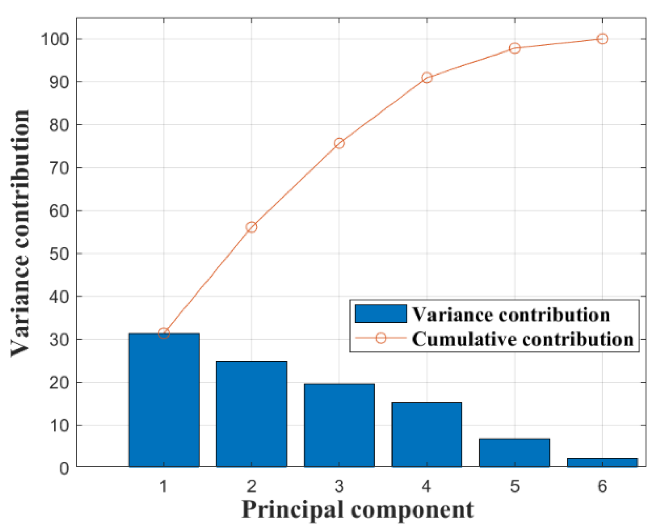
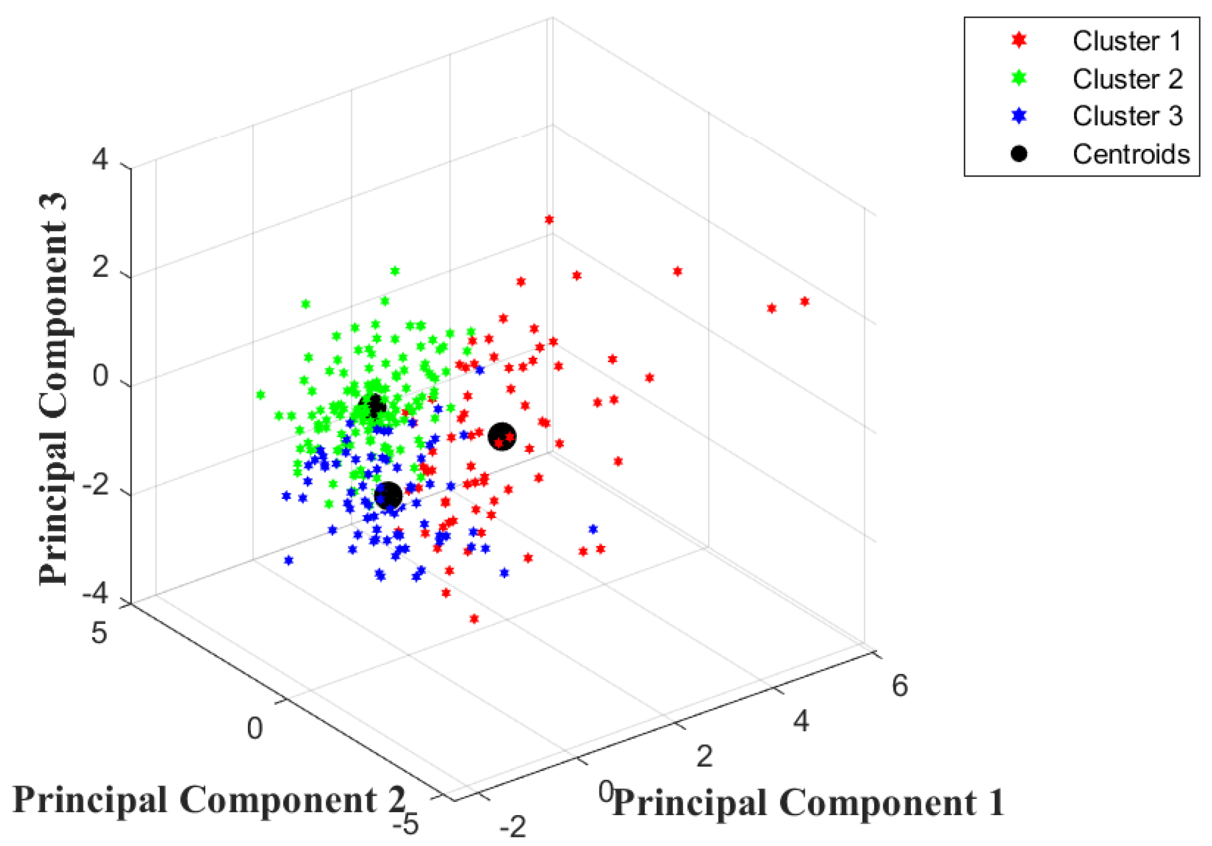
After the sample data were analyzed by PCA downscaling and K-means clustering analysis, the inputs of the driving style model were the top 4 principal component scores $\left[Y_1,Y_2,Y_3,Y_4\right]$ with a cumulative variance contribution rate greater than 85%, and the clustering result dataset of the K-means clustering analysis was the output of the model. In order to ensure that the neural network can fully learn the features and patterns of the data, 70% of the data is classified as the training data of the neural network, and the remaining 30% is classified as the test data of the neural network. To ensure the validity of the test data and enhance the accuracy of the model’s recognition, the selection of data samples was determined based on the outcomes of the K-means clustering analysis. Specifically, the sample set is composed of 25% radical data, 49% ordinary data, and 26% conservative data.

MATLAB is used to simulate and analyze the ACO-BP driving style recognition model, and the errors and accuracies of the simulated model are shown in

Table 7. Simulation results of the driving style model.

Model	MAE	MSE	RMSE	Recognition Accuracy
BP	0.1222	0.1444	0.38006	90%
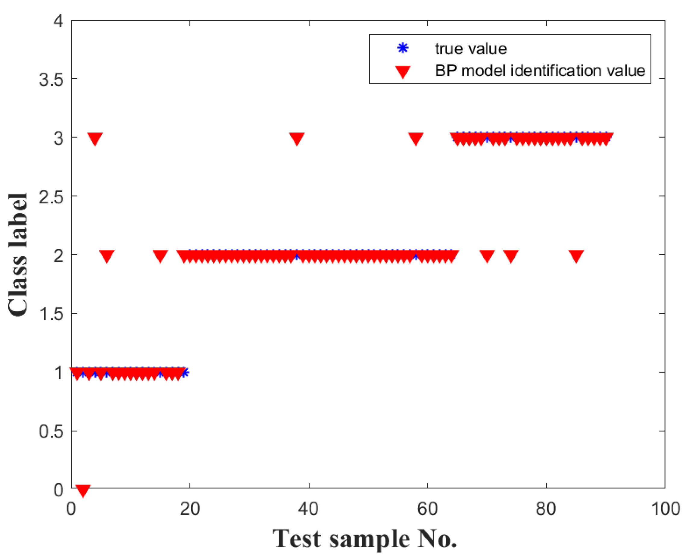
ACO-BP	0.0333	0.0333	0.1937	96.7%

. The ACO-BP model achieves a recognition accuracy of 96.7%, showing a significant improvement of 6.7% compared to the BP model’s recognition accuracy of 90%. The errors of the ACO-BP model are smaller than those of the BP model, and the accuracy of recognition surpasses that of the BP model. The simulation results comparing the recognition errors of the BP model and the ACO-BP model are shown in Figure 8. It is evident that the optimized model has fewer error points, resulting in smoother graphs. The error values of all points tend to be closer to 0.

The ACO-BP driving style recognition model has a clear advantage in terms of the overall error of the two models, with higher recognition accuracy. However, according to the relevant research, due to the more uncertain and dangerous driving behavior of aggressive-style drivers, they have significantly higher accident rates than the other two driving styles. Therefore, at the same time, the ACO-BP model is required to recognize the effect of each driving style and cannot have a large error in order to prevent the overfitting problem.

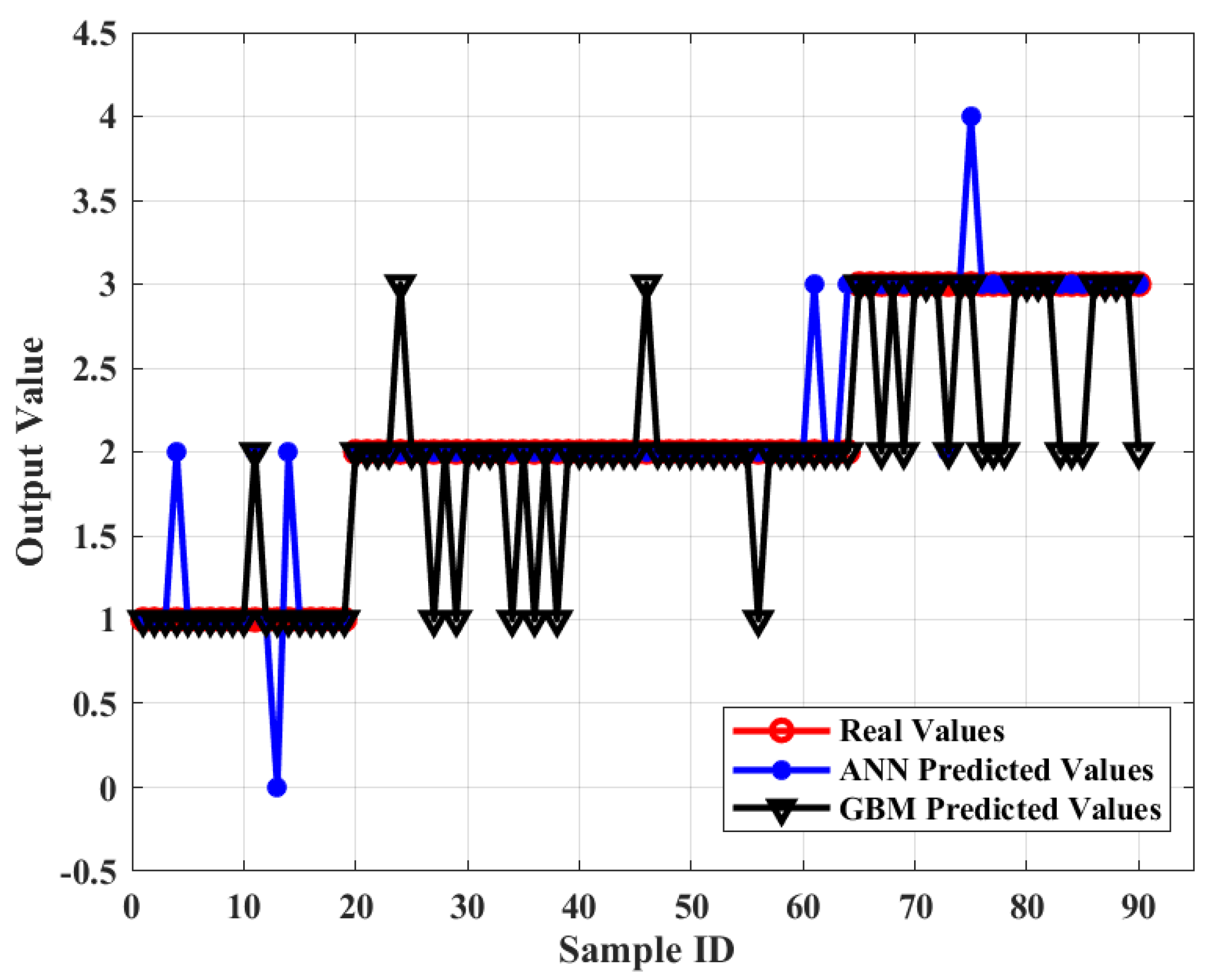
To further investigate the model’s effectiveness in recognizing driving styles in a more detailed manner, individual simulations are conducted to examine the impacts of identifying the three driving styles. The simulation results are shown in Figure 9 and Figure 10, which clearly show that the ACO-BP model has only 1, 0, and 2 samples producing recognition errors for each of the three driving styles of aggressive, ordinary, and conservative, respectively, while the BP model has 4, 2, and 3 samples producing recognition errors for each of the three driving styles, respectively. This indicates that, more than just the overall error, the ACO-BP model has better recognition accuracy than the BP model. When targeting different types of driving styles, the ACO-BP model is able to perform good recognition, and the recognition accuracy does not vary greatly due to the change in driving styles.

The specific recognition accuracy results for the 3 driving styles are shown in

Table 8. Model recognition accuracy of different driving styles.

Model	Aggressive	Ordinary	Conservative
BP	81.8%	95.6%	87%
ACO-BP	95.5	100%	91.3%

, which shows that for different driving styles, the recognition accuracy of the ACO-BP model is higher than that of the BP model. For the three driving styles of aggressive, normal, and conservative, the recognition accuracies are much improved, respectively: 13.7%, 4.4%, and 4.3%. It further proves the recognition accuracy and recognition value reliability of the ACO-BP model, and the recognition effect has obvious advantages for such an accident-prone driving population as the aggressive type.

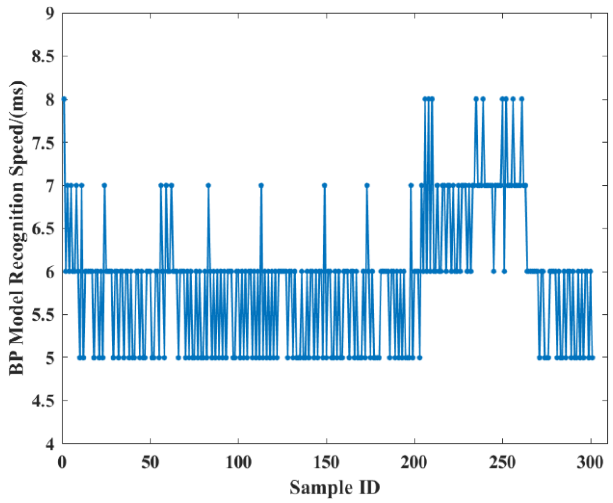
The driving style recognition speeds of the BP driving style recognition model and the ACO-BP driving style recognition model are shown in Figure 11 and Figure 12, respectively. The slowest recognition speed for the BP driving style recognition model is 8 ms, and the fastest recognition speed is 5 ms. For the ACO-BP driving style recognition model, the slowest recognition speed is 7 ms, and the fastest recognition speed is 5 ms, with a relatively uniform distribution within the range. The results indicate that, although ACO-BP is a hybrid model, it has not been significantly affected, as the recognition speed remains fast. Compared to the BP model, the recognition speed of the ACO-BP model is more even, and the speed range is more compact. Therefore, the ACO-BP driving style recognition model demonstrates better real-time performance compared to the BP driving style recognition model, enabling better adaptation to the actual road conditions of autonomous vehicles. It allows for timely recognition of driving styles, the avoidance of hazardous driving behaviors, and the improvement of driving safety.

5. Discussions

The comparison of the ACO-BP driving style recognition model with the BP driving style recognition model alone yields relatively limited results. Therefore, the artificial neural network (ANN) driving style recognition model and the gradient boosting machine (GBM) driving style recognition model were introduced to compare accuracy and real-time performance. The simulation results are shown in Figure 13. It can be observed that, compared to the ACO-BP model’s three error points, the ANN model has eight error points, and the GBM model has 18 error points. The ACO-BP model exhibits significantly fewer errors in sample recognition in comparison to the ANN and GBM models. This indicates that the ACO-BP model possesses a greater advantage in terms of recognition accuracy, enabling better differentiation of driving styles. The chances of avoiding aggressive driving styles are enhanced, which ensures better road safety in autonomous driving.

The driving style recognition speeds of the artificial neural network (ANN) driving style recognition model and gradient boosting machine (GBM) driving style recognition model are shown in Figure 14 and Figure 15, respectively. The slowest recognition speed for the ANN model is 9 ms, while the fastest recognition speed is 5 ms. On the other hand, the fastest recognition speed for the GBM model is 10 ms, whereas the slowest recognition speed is 7 ms. Compared to the ANN model, the GBM model exhibits relatively slower recognition speed.

In this paper, the recognition accuracy and speed ranges of the four driving style recognition models mentioned are shown in

Table 9. Recognition results of driving styles for each model.

Model	Recognition Accuracy	Recognition Speed Range (ms)
ACO-BP	96.7%	[5,7]
BP	90%	[5,8]
ANN	91.11%	[5,9]
GBM	80%	[7,10]

. First, in terms of recognition accuracy, the ACO-BP model has the highest recognition accuracy, significantly higher than the other three driving style recognition models. This ensures the ability of autonomous vehicles to accurately distinguish risky driving behaviors and timely avoid driving risks. Secondly, the recognition speed range of the ACO-BP model is close to that of the BP model, and it is the lowest among the four models. However, by observing the simulation results of the recognition speed of the four models, it is evident that the recognition speed range distribution of the ACO-BP model is the most uniform, with most samples having a recognition speed of 5 ms or 6 ms and only a small number of samples having a recognition speed of 7 ms. This ensures the real-time recognition of driving styles for autonomous vehicles, allowing them to make the fastest recognition while driving on actual roads.

6. Conclusions

To summarize, the key findings of this research are:

• Through principal components analysis and K-means clustering analysis, it was found that when driving styles were divided into three classes, the clustering effect was better, and there was no underclassification or overclassification problem.
• The model error simulation results before and after ACO show that the ACO-BP model demonstrates superior overall recognition accuracy compared to the BP model, indicating that the recognition accuracy of the ACO-BP driving style recognition model was improved and the reliability was better.
• The recognition effect of the ACO-BP and BP driving style recognition models on different driving styles shows that, in terms of classification and recognition accuracy, the ACO-BP model has a better classification and recognition effect than the BP model, especially for aggressive-type accident-prone people, and the accurate recognition of this kind of driving style is conducive to the timely avoidance of risks.
• To further verify the identification accuracy and real-time performance of the ACO-BP model, the ANN and GBM models are introduced. The results demonstrate that the ACO-BP model achieves optimal identification accuracy and real-time recognition speed.

In general, the ant colony optimization of the BP neural network demonstrates higher reliability in autonomous driving style recognition. However, due to the limitations of setting conditions when screening the data, the sample data is small, and the driving style recognition results are poor in macroscopic. The following research will incorporate practical autonomous vehicles to conduct identification experiments in various road environments and optimize the system accordingly.

References

1. Khan, M.A. Intelligent Environment Enabling Autonomous Driving. IEEE Access 2021, 9, 32997–33017. [Google Scholar] [CrossRef]
2. Malik, S.; Khan, M.A.; El-Sayed, H.; Khan, J.; Ullah, O. How Do Autonomous Vehicles Decide? Sensors 2023, 23, 317. [Google Scholar] [CrossRef] [PubMed]
3. Afandizadeh, S.; Sharifi, D.; Kalantari, N.; Mirzahossein, H. Using machine learning methods to predict electric vehicles penetration in the automotive market. Sci. Rep. 2023, 13, 312–326. [Google Scholar] [CrossRef] [PubMed]
4. Li, X.S.; Zhang, Q.S.; Song, C.Q.; Kang, Y.H.; Cheng, J. Review of Trajectory Prediction Techniques Under Autonomous Driving Scenarios. J. Comput. Eng. 2023, 49, 1–11. [Google Scholar]
5. Kim, K.; Kim, J.S.; Jeong, S.; Park, J.H.; Kim, H.K. Cybersecurity for autonomous vehicles: Review of attacks and defense. Comp. Security 2021, 103, 102150. [Google Scholar] [CrossRef]
6. Szarata, A.; Ostaszewski, P.; Mirzahossein, H. Simulating the impact of autonomous vehicles (AVs) on intersections traffic conditions using TRANSYT and PTV Vissim. Innov. Infrastruct. Solut. 2023, 8. [Google Scholar] [CrossRef]
7. Ge, H.M.; Huang, W.K.; Zang, W.K.; Dong, L.; Zhou, L.J. Research on driving style recognition model considering driver-environment interaction. J. Chongqing Univ. Technol. 2023, 37, 1–10. [Google Scholar]
8. Li, Z.H.; Wu, C.; Tao, P.F.; Tian, J.; Ma, L. Dp&ds-lcd: A new lane change decision model coupling driver’s psychology and driving style. IEEE Access 2020, 8, 132614–132624. [Google Scholar] [CrossRef]
9. Dang, J.J.; Wang, L.J. Optimization control of hydrogen engine ignition system based on ACO-BP. Int. J. Hydrogen Energy 2021, 46, 38903–38912. [Google Scholar] [CrossRef]
10. Jeyaraj, R.; Paul, A. Optimizing MapReduce Task Scheduling on Virtualized Heterogeneous Environments Using Ant Colony Optimization. IEEE Access 2022, 10, 55842–55855. [Google Scholar] [CrossRef]
11. Ru, Q.J.; He, Z.L.; Yang, J.C.; Li, X.L.; Tan, J.B. Research on ACO-BP Neural Network-Based Displacement Monitoring Model for Soil and Rock Dams. J. Water Resour. Water Eng. 2020, 30, 196–201. [Google Scholar]
12. Kumar, R.; Jain, A. Driving behavior analysis and classification by vehicle OBD data using machine learning. J. Supercomput. 2023, 79, 18800–18819. [Google Scholar] [CrossRef] [PubMed]
13. Peng, J.S.; Zhao, W.Q.; Liu, L.; Liu, T.; Zhang, L. Driving Style Recognition and Transferability Analysis of Stable Following State. J. Chongqing Jiaotong Univ. 2023, 42, 106–113. [Google Scholar]
14. Zhao, L.; Xu, T.; Zhang, Z.S.; Hao, Y. Lane-Changing Recognition of Urban Expressway Exit Using Natural Driving Data. Appl. Sci. 2022, 12, 9762. [Google Scholar] [CrossRef]
15. Mirzahossein, H.; Gholampour, I.; Sajadi, S.R.; Zamani, A.H. A hybrid deep and machine learning model for short-term traffic volume forecasting of adjacent intersections. IET Intell. Transp. Syst. 2022, 16, 1648–1663. [Google Scholar] [CrossRef]
16. Milardo, S.; Rathore, P.; Santi, P.; Ratti, C. A Data-Driven Framework for Driving Style Classification. In Proceedings of the 18th International Conference on Advanced Data Mining and Applications (ADMA), Brisbane, Australia, 28–30 November 2022. [Google Scholar]
17. Bejani, M.M.; Ghatee, M. Convolutional Neural Network with Adaptive Regularization to Classify Driving Styles on Smartphones. IEEE Trans. Intell. Transp. Syst. 2019, 21, 543–552. [Google Scholar] [CrossRef]
18. Xu, J.W.; Pan, S.C.; Sun, Z.H.; Park, S.H.; Guo, K. Human-Factors-in-Driving-Loop: Driver Identification and Verification via a Deep Learning Approach using Psychological Behavioral Data. IEEE Trans. Intellig. Trans. Syst. 2023, 24, 3383–3394. [Google Scholar] [CrossRef]
19. Liang, K.C.; Zhao, Z.G.; Li, W.C.; Yan, D. Comprehensive Identification of Driving Style Based on Vehicle’s Driving Cycle Recognition. IEEE Trans. Veh. Technol. 2023, 72, 312–326. [Google Scholar] [CrossRef]
20. Zhang, H.; Zhang, Z.Y.; Liang, J. Dynamic driving intention recognition of vehicles with different driving styles of surrounding vehicles. IET Intell. Transp. Syst. 2022, 16, 571–585. [Google Scholar] [CrossRef]
21. Cai, Y.F.; Zhao, R.D.; Wang, H.; Chen, L.; Lian, Y.; Zhong, Y. CNN-LSTM Driving Style Classification Model Based on Driver Operation Time Series Data. IEEE Access 2023, 11, 16203–16212. [Google Scholar] [CrossRef]
22. Kim, D.; Shon, H.; Kweon, N.; Choi, S.; Yang, C.; Huh, K. Driving Style-Based Conditional Variational Autoencoder for Prediction of Ego Vehicle Trajectory. IEEE Access 2021, 9, 169348–169356. [Google Scholar] [CrossRef]
23. Huang, F.C.; Liu, D.X.; Cao, J.; An, T.S. Ship traffic flow prediction based on ABC optimized BP neural network. China Navig. 2021, 44, 78–83. [Google Scholar]
24. Tang, C.L.; Zhao, Y.Q.; Liu, X.Y. Structural design of two-dimensional multilayer subwavelength gratings based on ant colony algorithm. J. Infrared Millim. Waves 2022, 41, 756–761. [Google Scholar]
25. Ren, X.H.; Gou, L.Z.; Wu, T. UAV terminal delivery under uncertainty fault. J. Guangxi Univ. 2022, 47, 732–745. [Google Scholar]
26. Yang, C.H.; Zheng, L.; Zuo, Y.F.; Wang, K.; Zeng, J.; Ding, X.C. Research on lane-changing driving behaviors based on highway scenarios. J. Chongqing Univ. 2023, 1–16. Available online: https://kns.cnki.net/kcms/detail/50.1044.N.20230620.0946.002.html (accessed on 1 November 2023).
27. Li, G.; Zhai, W.; Huang, H.B.; Ren, J.L.; Wang, D.Z.; Wu, G. Behavioral model for confluence decision-making based on multiple adaptive regression spline. J. Tsinghua Univ. 2023, 1–8. [Google Scholar]
28. Xu, L.F. Research on Intelligent Vehicle Following Based on Machine Learning. Master’s Thesis, Anhui University of Engineering, Wuhu, China, 2022. [Google Scholar]
29. Kim, D.J.; Kim, J.S.; Yang, J.H.; Kee, S.C.; Chung, C.C. Lane Change Intention Classification of Surrounding Vehicles Utilizing Open Set Recognition. IEEE Access 2021, 9, 57589–57602. [Google Scholar] [CrossRef]
30. Toledo, T.; Koutsopoulos, H.N.; Ahmed, K.I. Estimation of vehicle trajectories with locally weighted regression. Transp. Res. Rec. 2007, 1999, 161–169. [Google Scholar] [CrossRef]
31. Zhang, Y.D. Game Model of Vehicle Lane Changing Behaviors Based on NGSIM Data. Master’s Thesis, Beijing Jiaotong University, Beijing, China, 2016. [Google Scholar]
32. Hu, C.Y.; Qu, D.Y.; Zhao, Z.X.; Song, H.; Wang, T. Improved adaptive cruise control following model and simulation considering the driving style of the vehicle in front. J. Jinan Univ. 2023, 37, 331–338. [Google Scholar]
33. Aldibaja, M.; Suganuma, N.; Yoneda, K. Robust Intensity-Based Localization Method for Autonomous Driving on Snow-Wet Road Surface. IEEE Trans. Ind. Inform. 2017, 13, 2369–2378. [Google Scholar] [CrossRef]
34. Sun, X.F.; Zhao, Y.; Lv, C.M. Influence Mechanism of Human-Computer Interaction Trust in Autonomous Vehicles. J. Northeast Univ. 2022, 9, 1305–1313. [Google Scholar]
35. Liu, B.X.; Zhang, H.Y.; Wang, M.; Wu, H.; Zong, F. Study on human driving behaviors when following an autonomous vehicle: Empirical evidence and modelling. J. Transp. Eng. Inf. 2023, 21, 14–28. [Google Scholar]
36. Das, A.; Khan, M.N.; Ahmed, M.M.; Wulff, S.S. Cluster analysis and multi-level modeling for evaluating the impact of rain on aggressive lane-changing characteristics utilizing naturalistic driving data. J. Transp. Saf. Secur. 2022, 14, 2137–2165. [Google Scholar] [CrossRef]
37. Huang, J.; Li, Y.H.; Wu, S.B.; Ding, D.L.; Luo, H.; He, Y. A study on driving style recognition based on multivariate feature parameters and improved SVM algorithm. J. Chongqing Univ. Technol. 2022, 36, 8–19. [Google Scholar]
38. Tang, C.Y.; Zhang, M.L.; Li, J.H.; Wan, Y.; Wei, M.R. Research on takeaway delivery path planning based on improved ant colony algorithm. J. Nanjing Univ. Inform. Eng. 2023, 1–14. [Google Scholar] [CrossRef]
Figure 1. Structure of the BP neural network.
Applsci 13 12367 g001
Figure 2. Flowchart of the ACO-BP algorithm.
Applsci 13 12367 g002
Figure 3. Vehicle speed smoothing effects. (a) Global view of the speed smoothing effect; (b) smoothing effect of vehicle speed in 10 s before and after lane changing.
Applsci 13 12367 g003
Figure 4. Acceleration smoothing effects. (a) Global view of the acceleration smoothing effect; (b) acceleration smoothing effect in 10 s before and after lane changing.
Applsci 13 12367 g004
Figure 5. Contribution rate graph.
Applsci 13 12367 g005
Figure 6. K-means clustering effect.
Applsci 13 12367 g006
Figure 7. Evolutionary convergence curve.
Applsci 13 12367 g007
Figure 8. Simulation results of the model error comparison before and after ACO optimization.
Applsci 13 12367 g008
Figure 9. Effect of different driving styles recognized by the BP model.
Applsci 13 12367 g009
Figure 10. Effect of different driving styles recognized by the ACO-BP model.
Applsci 13 12367 g010
Figure 11. Driving style recognition speed of the BP model.
Applsci 13 12367 g011
Figure 12. Driving style recognition speed of the ACO-BP model.
Applsci 13 12367 g012
Figure 13. Prediction results of the ANN and GBM driving style recognition models.
Applsci 13 12367 g013
Figure 14. Driving style recognition speed of the ANN model.
Applsci 13 12367 g014
Figure 15. Driving style recognition speed of the GBM model.
Applsci 13 12367 g015