Study of the Reasonable Acquisition Frequency Evaluation Method of Midspan Deflection of Medium- and Small-Span Beam Bridges

Abstract

The objective of this study is to further promote and apply the structural monitoring system to medium and small bridges, given the relative delays in scientific research, technical specifications, and engineering practice for the safety monitoring of small and medium-span girder bridges, as well as the relative simplicity of the structural system of these bridges, their well-defined forces, and the relatively large proportion of live load responses during operation. These concepts are proposed based on the evaluation method of live loading (As therefore, this paper suggests the notion of sensor acquisition frequency and appropriate acquisition frequency based on the live load assessment method and the fundamental reliability theory). Based on the time-history curve depicting the midspan deflection response of the vehicle-bridge coupling system, the frequency domain analysis reveals that the power spectrum at −3 dB corresponds to the response cutoff frequency. Significantly, the cutoff frequency mentioned is double the acquisition frequency considered suitable for the study. Based on the definition of a quasi-static response, it can be deduced that the velocity of a load does not exert any influence on the quasi-static response of a bridge structure. As a result, the derivation of the components related to the midspan deflection of a bridge’s quasi-static response is presented, together with a recommended set of methodological guidelines for the extraction of finite elements. This study introduces a novel approach for determining the cutoff frequency of the structural response by utilizing the characteristics of amplitude spectrum estimation and power spectrum estimation in frequency domain analysis. The cutoff frequency of the signal is determined by analyzing the amplitude-frequency curve of the power spectrum. Subsequently, the probability density function of the original time-history curve data is estimated based on the amplitude spectrum. Finally, reliability analysis is conducted by calculating the ratio of the amplitude spectrum area of the signal obtained through a reasonable acquisition frequency to the area of the amplitude spectrum function of the original signal. This analysis verifies the reliability of the proposed method for determining the midspan deflection acquisition frequency.

1. Introduction

Small- and medium-span beam bridges possess a straightforward structural system, exhibit evident stress patterns, and demonstrate substantial responsiveness to live loads during their operational lifespan. As a result, live load monitoring data are commonly used in health monitoring and evaluation procedures [1,2,3].

The prevailing bridge health monitoring system generally functions with the presumption that the constant frequency data acquired from sensors can faithfully depict the true state of deformation exhibited by the structure. Nevertheless, the structural deformation of the bridge experiences ongoing fluctuations. Equal frequency acquisition denotes a discrete process in which data are continuously deformed. However, this approach is not without its limitations, including issues such as the absence of crucial data points and the distortion of curves. Research has shown that the experimental fundamental frequency has been used to predict the prestress losses in simply supported concrete bridges [4,5]. This measurement has the potential to provide dependable insights into the current prestress losses experienced by concrete girder-bridges undergoing significant fracture. In the context of small- and medium-span beam bridges, it is noteworthy that the live load component constitutes a significant portion of the overall design load, with estimates indicating that it may even reach approximately 50.0% [6]. Therefore, it is crucial to obtain exhaustive influence data regarding the response of the structure to real-world loads, in addition to meticulously determining the optimal sampling frequency for the monitoring system’s sensors. Insufficiently setting the acquisition frequency can result in a decrease in the amount of acquired data, a potential compromise in capturing key points, and even the possibility of missing responses. Setting the acquisition frequency excessively high can result in substantial data accumulation, thereby necessitating greater hardware investment and posing challenges in data analysis [7,8].

After conducting a thorough examination of the available data on frequency settings for small- and medium-span beam bridges both domestically and internationally, it has been observed that there is a scarcity of research in this area. The analysis of the data can be summarized as follows: Stiros et al. [9] tested the structural dynamic characteristics of Gorgopotamos bridge, and calculated that the midspan deflection of the structure caused by heavy freight trains crossing the bridge is about 6 mm and the frequency range of the structure is between 3.18 and 3.63 Hz; José Venâncio Marra de Oliveira [10,11] used a 100 Hz GPS to dynamically monitor a small concrete bridge, and used a CWT-Morlet filter to provide accurate position transient signal and report the fundamental frequency of the structure at the same time. The filtered data were displayed on the identification scale diagram, and it was found that the confidence level was 95.0% and the frequency range was 0.1 to 50 Hz. Li et al. [12] put forward the method of frequency conversion acquisition, using radar sensors to identify the height of the car body, and then determine whether to adopt high-frequency acquisition in order to achieve the purpose of the real-time online monitoring of bridge deflection by vehicle control. The analysis involves utilizing a three-span continuous beam bridge with a length of 180 m. The bridge’s fundamental frequency is determined to be 1.645 Hz. To capture high-frequency data, a frequency of 20 Hz is chosen for acquisition. Similarly, a frequency of 0.1 Hz is selected for acquiring low-frequency data. By employing these frequencies, the response of the entire vehicle crossing process on the bridge is obtained. While it is possible to observe abnormal deflection and deformation, the reliability of the collected data is still a subject of debate.

In addition, Pourzeynali S et al. [13] studied the influence of acquisition frequency on the accuracy of the Newmark-β method. The average speed of vehicles crossing the bridge was 0.47 m/s, and the acquisition frequency was set to 600 Hz and re-acquired at 300 Hz, 200 Hz, and 100 Hz, respectively, so as to obtain the influence of different acquisition frequencies. The outcomes of relocating loads that were detected using various acquisition frequencies exhibited variations, and the precision of identification was assessed based on the strain error observed during midspan reconstruction. The findings indicate that the proposed method effectively detects the dynamic load across various frequency ranges of data acquisition. While it is true that increasing the frequency of acquisition can lead to a slight improvement in reconstruction strain, it also results in a significant increase in recorded data and a longer analysis time, which is not considered desirable. At present, the acquisition frequency of GPS at home and abroad can reach 100 Hz, but it is usually only 10–20 Hz in practical structural engineering, and it is easily affected by environmental factors, such as noise [14]. For the contact LVDT [15] (linear variable differential transducer) or the tension line, the maximum acquisition frequency can reach 100 Hz. In practical engineering, the frequency used in the monitoring system is mainly 1–2 Hz, and the acquisition should also meet the requirements of real-time alarm, data analysis, and application.

In summary, in view of the small- and medium-span girder bridges all over the highway traffic network, there is no reasonable collection frequency assessment method, and so the study will be based on the probabilistic integral method of structural reliability and the signal analysis method, and put forward a simpler, applicable, and reasonable collection frequency setting method, in order to provide relevant bases for the optimization of the health monitoring and analysis methods of small- and medium-span girder bridges.

2. Acquisition Frequency and Reasonable Acquisition Frequency

When the health monitoring system has been deployed, discrete data extraction from the system’s continuously generated signals constitutes the majority of the work required to obtain bridge structure information. The frequency at which this acquisition occurs serves as an indicator of the effectiveness of signal capture to a certain degree. Therefore, a reasonable acquisition frequency is very important to judge the bridge state by using the change in live load response, and different acquisition frequencies will lead to different integrities of monitoring data [16,17]. In view of the sensor’s performance, data storage capacity, field installation, and other practical conditions, and for the sake of cost, it is usually desirable to obtain the response of the bridge structure with a smaller acquisition frequency [18]. Consequently, in order to facilitate the dynamic monitoring of bridge structures, it is necessary to investigate the feasibility of capturing the true response process of the structure with a lower acquisition frequency and the determination of an appropriate acquisition frequency.

The acquisition frequency of a bridge structure can be defined by: Measuring the value of the continuous responses in units at intervals. The unit acquisition process produces a series of numbers, called samples. The response of the original structure is replaced by samples for analysis. Among them, the reciprocal of the acquisition interval (1/T) is the acquisition frequency (f_s), and its unit is sample/second, that is, hertz (Hz). According to the Nyquist sampling theorem, the reasonable acquisition frequency is defined as twice the cutoff frequency of the structural response [19], as shown in Figure 1.

The traditional cutoff frequency selection process is that the original time series is Fourier transformed to obtain the frequency spectrum, and then a position between the two poles is found in the frequency spectrum and the frequency value corresponding to this position can be used as the selected cutoff frequency [20,21]. The traditional selection method of cutoff frequency depends on the spectrogram. Once the spectrogram is distorted or too complicated, it is difficult to find the accurate cutoff frequency [22]. For small- and medium-span, simply supported beam bridges, Li Weizhao [23] put forward a method based on modern dynamic signal analysis theory to extract the maximum static response of the bridge. By approximating the effect of moving vehicles on the bridge as the superposition of the moving constant force and the moving harmonic force, this method carries out spectrum analysis on the dynamic response of the bridge, and selects the right valley value of the first main lobe of the power spectrum as the cutoff frequency, thus determining the frequency band of the static component in the bridge vibration response; Gao Liming [24] regarded the fast response pressure sensitive paint as a “dynamic pressure sensor”. In order to obtain an effective working frequency, a series of studies have found that if the signal amplitude gain > −3 dB, the corresponding frequency is the cutoff frequency, which can better reflect the dynamic change in pressure, otherwise, the measurement result will be distorted. Chen Xiaodong [25] monitored a long-span PC beam in Guangzhou in real time by total station, and obtained the midspan deflection time-history curve. According to the probability analysis method in the reliability theory, the acquisition frequency at a 95.0% assurance rate was determined as a reasonable value.

In conclusion, this article defines the cutoff frequency of the structural response signal of a bridge. The cutoff frequency is defined as the extent to which the deflection response efficiently functions within a particular frequency range, contingent upon the structural response undergoing a specific amplitude change and meeting the effective resolution criteria. This is specifically observed through the Fourier transform of the response time-history curve, which allows for the determination of the frequency at which the signal amplitude gain reaches −3 dB, thus establishing the “cutoff frequency” of the signal. Furthermore, the conventional approach for selecting the cutoff frequency may result in inaccuracies during signal decomposition. A proposed method is introduced to enhance the accuracy of selecting the cutoff frequency for signal decomposition. This method utilizes a power spectrum-based approach to determine the appropriate acquisition frequency for the structure. The distinction lies in the fact that the reasonable value primarily reconstructs the quasi-static response signal of the acquired signal based on reliability theory [25,26], thereby approximating the peak point.

3. Quasi-Static Component of Deflection Response and Its Extraction

The concept of a quasi-static response is introduced so that the feasibility of the evaluation method for reasonable acquisition frequency can be investigated further [27]. The quasi-static response of a vehicle-bridge coupled vibration system [28,29,30,31,32,33] pertains to the response of the bridge structure as the vehicle’s velocity perpetually approaches zero. Therefore, the quasi-static response of the bridge is not affected by the moving speed of the load; on the contrary, the moving speed of the load will not cause a change in quasi-static components. It is assumed that there is no displacement and speed at the beginning of beam vibration, and the midspan deflection response of a simply supported beam bridge under moving load is divided into moving the load frequency component $u_m$ and the bridge natural vibration frequency component $u_n$. Accordingly, it can be deduced that the component controlled by the natural vibration frequency ${\omega }_i$ of the bridge is zero, and the frequency component of the moving load is mainly controlled by the excitation frequency $i\pi \nu /L$ of the external load, which can be expressed as shown in (1):

$$u_m=\frac{2F}{\rho AL}\sum _{i=1}^n\frac{1}{{\omega }_i(1-S_i^2)}\mathit{sin}\frac{i\pi vt}{L}\mathit{sin}\frac{i\pi x}{L}$$

(1)

where $S_i$ is a dimensionless speed parameter, and it is the ratio of the i—order moving load frequency to the i—order bridge natural vibration frequency, which can be expressed as $i\pi \nu /L{\omega }_i$.

In practical engineering, when the speed parameter is equal to 1, the bridge structure will resonate with the vehicle load, which will easily cause structural damage. He et al. [34], according to the statistics of natural frequencies of highway bridges, determined that the reasonable range for dimensionless speed parameters $S_i$ is between 0 and 0.15.

For the deflection response, when the moving speed of the vehicle is infinitely close to zero, the moving load can be approximately regarded as a quasi-static load, and the dimensionless speed parameter $S_i=0$ can be further derived, and the quasi-static component $u_{st}$ of the bridge response can be expressed as shown in (2):

$$u_{st}=\frac{2F}{\rho AL}\sum _{i=1}^n\frac{1}{{\omega }_i}\mathit{sin}\frac{i\pi \overline{x}}{L}\mathit{sin}\frac{i\pi x}{L}$$

(2)

where, $\overline{x}=vt$ represents the position where the quasi-static load acts, and $u_{st}$ represents the deflection response at measuring point $x$ when the static load acts on $\overline{x}$.

The quasi-static response is mainly concentrated in the low-frequency section of the overall dynamic response [35]. It is assumed that the discrete signal $x\left(t\right)$ obtained after continuous signal $x\left(n\right)$ acquisition can be in the form of a series of harmonic superposition, and the expression is shown in (3):

$$x\left(n\right)=\sum a_i\mathit{cos}\left({\omega }_i\cdot n\cdot \mathsf{\Delta }t+{\phi }_i\right)$$

(3)

where, $a_i$, ${\omega }_i$, and ${\phi }_i$ represent the amplitude, frequency, and initial phase of the $i$ th harmonic, respectively; where $\mathsf{\Delta }t=1/f_s$ is the acquisition interval.

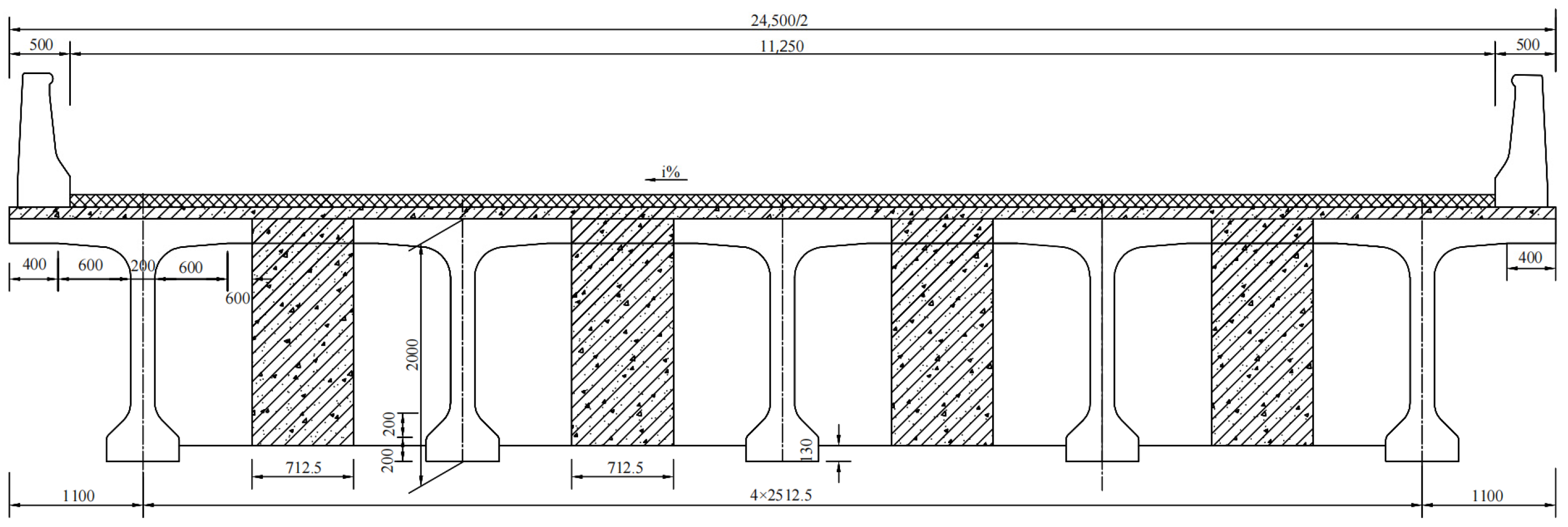
The dynamic response of a bridge caused by a moving load includes not only quasi-static components, but also signal components caused by natural bridge vibration, vehicle speed, noise, and other factors. It is difficult to directly and clearly observe the quasi-static components. Therefore, it is necessary to use a method to extract quasi-static components from the dynamic response of the bridge structure. In this case, the data obtained from the side span of a simply supported T-beam bridge with a 30-m span are analyzed as an example, while the vehicle travels through the side beam. The superstructure and section dimensions are illustrated in Figure 2, Figure 3, Figure 4 and Figure 5.

The performance of various materials is shown as follows: (1) C50 (high-performance concrete) is used for precast main girders and diaphragm girders, wet joints, sealing and anchoring ends, and cast-in-place continuous sections on top of piers; (2) C50 (high-performance concrete) is used for cast-in-place concrete of the bridge decks; (3) asphalt concrete is used for bridge deck paving; (4) Reinforcing steel mainly adopts HPB300 and HRB400; (5) A seven-wire twisted standard-type low relaxation high-strength strand is adopted, with a nominal diameter of 15.20 mm, a nominal area of 140 mm², a tensile standard strength of ${\mathrm{f}}_{\mathrm{pk}}=1860\mathrm{MPa}$, a modulus of elasticity of ${\mathrm{E}}_{\mathrm{P}}=1.95 \times {10}^5\mathrm{MPa}$, and a maximum relaxation rate of 3.5%.

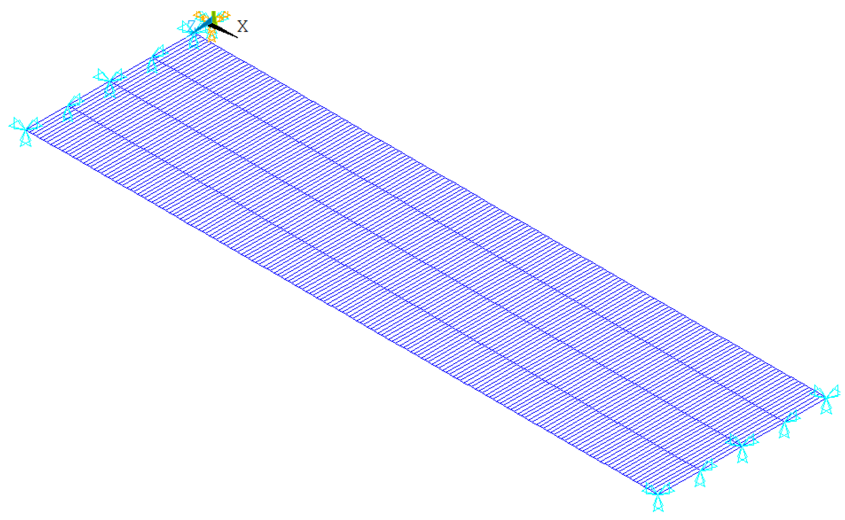
For the finite element simulation, ANSYS was used to establish the finite element model of the bridge, and a BEAM4 element was used to simulate the main beam, a MASS21 element was used to simulate the mass, as well a COMBIN14 spring element. The finite element model of the bridge with a 30-m span simply supported T-beam is shown in Figure 6.

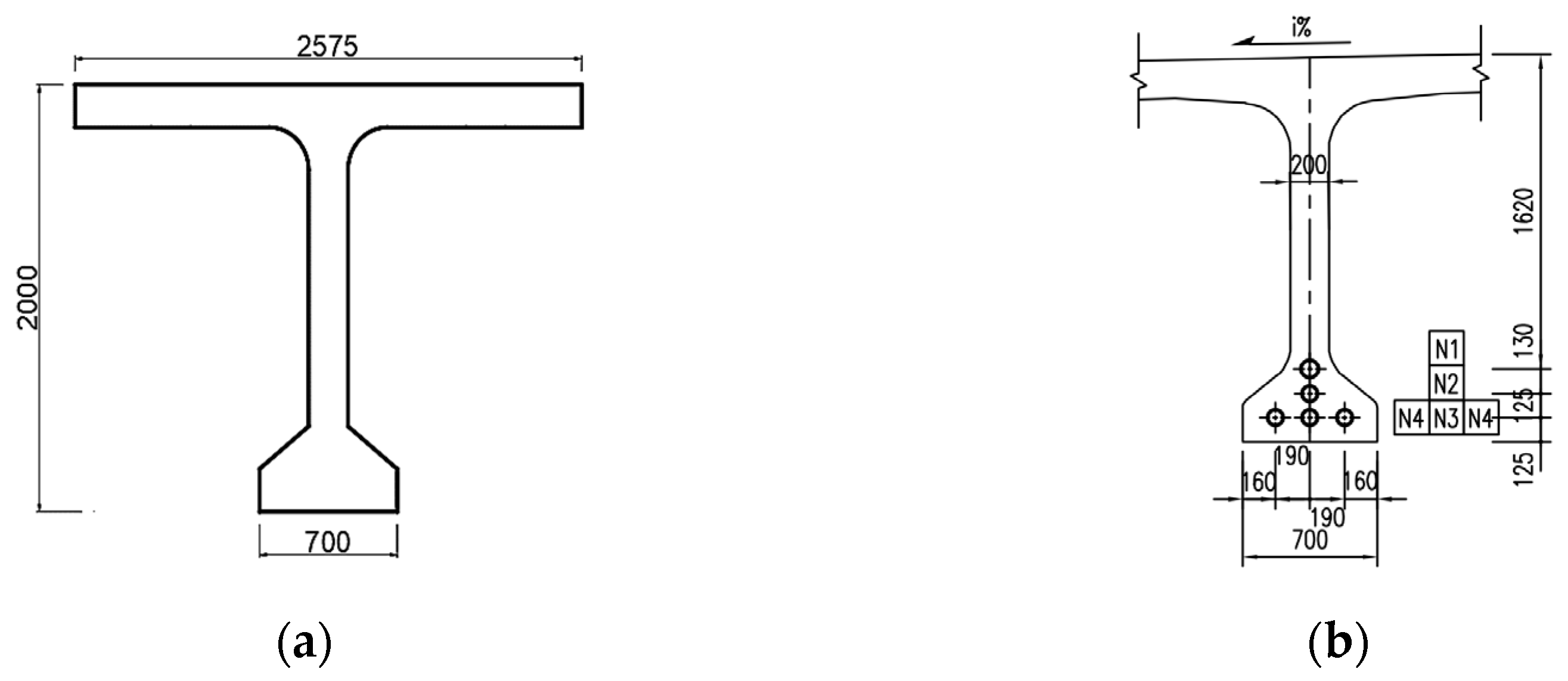
In this paper, the bridge structure adopts a BEAM4 unit, which is a common type of unit for main beam modeling. It is a 3D elastic beam unit with 6 degrees of freedom directions (UX, UY, UZ, ROTX, ROTY, ROTZ), which can withstand axial tension, pressure, bending moment, and torsion, and does not have the function of plasticity and eccentric force. Here, the mid-span section of a 30-m span simply supported T-beam is taken as an example. The section size and structure are shown in Figure 2, Figure 3, Figure 4 and Figure 5, using the International System of Units, and the specific values are shown in

Table 1. BEAM4 unit real constant.

Serial Number	Name	Numerical Value	Serial Number	Name	Numerical Value
1	AREA	0.806	7	ISRRN	-
2	Izz	0.276321	8	Ixx	0.0137968
3	Iyy	0.161184	9	SHEARz	-
4	Tkz	0.25	10	SHEARy	-
5	Tky	2	11	SPIN	-
6	THETA	-	12	ADDMAS	-

.

The moving mass block adopts the MASS21 unit, and each node has 6 degrees of freedom in each direction (UX, UY, UZ, ROTX, ROTY, ROTZ), and each coordinate direction has a different mass and moment of inertia. This type of unit can define the moment of inertia effect and the choice of 2D or 3D functions via KEYOPT(3).

Table 2. Geometric characteristics of section of simply supported T-beam.

Span	Category	Fulcrum Side Beam	Pivot Center Beam	Mid-Span Edge Beam	Midspan Beam
30 m	Principal moment of inertia (m4)	1.4401	1.4776	1.00512	1.0426
	Submoment of inertia (m4)	0.6615	0.6816	0.5294	0.5434
	Torsion moment of inertia (m4)	0.0851	0.0854	0.0201	0.0205

shows the relevant characteristics of a midspan cross-section and a fulcrum cross-section corresponding to the simple supported T-beam bridge with different spans, including the principal moment of inertia of the main beam, the secondary moment of inertia, and the torsional moment of inertia. Based on the analysis of the ANSYS modal calculation results, the first three natural vibration frequencies of simply-supported beam bridges with different spans under the bridge state were extracted and are drawn in

Table 3. Dynamic characteristics of bridge (Unit: Hz).

Order	1	2	3
30-m simple supported T-beam	4.302	6.938	8.049

.

For the finite element simulation, the specific operation steps for obtaining the midspan deflection time-history curve are as follows:

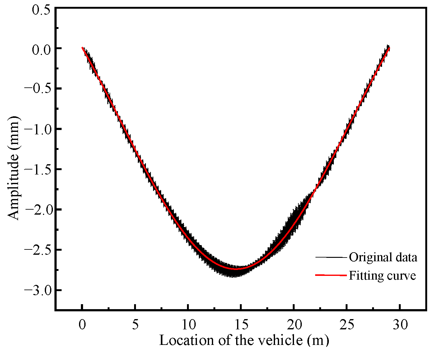
Step 1: Set the mass of the moving load, and keep driving on the bridge deck at low speed and at a uniform speed to obtain the midspan deflection time-history curve caused by the moving load;

Step 2: Because the moving speed is small, the amplitude of the time-history curve is small, so the GUASS curve fitting method is used to fit the static time-history curve; the fitting result is shown in Figure 7.

For historical response data, the specific operation steps are as follows:

In the first step, the frequency components of the moving load are extracted based on the Analytical Modal Decomposition (AMD) method, which can decompose multi-frequency signals into single-frequency signals [36]. Generally speaking, the speed parameters $S_i \le 0.15$ of bridge structures are generally dimensionless in the actual operation process, which shows that the natural vibration frequency of the first-order bridge is at least six times that of the same-order moving load [37]. Therefore, the moving load frequency and natural vibration frequency of the bridge can be separated from the frequency spectrum of the bridge response. Firstly, the Fourier transform is carried out on the deflection response curve of the bridge to obtain the frequency spectrum, and the cutoff frequency is estimated based on the amplitude spectrum or power spectrum. Then, the frequency component of the moving load is extracted from the original signal through a low-pass filter or other signal analysis tools.

Secondly, based on the Moving Average Filter (MAF) [38,39,40,41] filtering method, the high-frequency vibration caused by the speed factor is filtered out, and then the quasi-static components are extracted.

4. Frequency Estimation of Midspan Deflection Signal Acquisition

4.1. Frequency Characteristics of Bridge Deflection

Assuming that the highest frequency of the original signal is $f$, the mean value is $u$, the mean square value is ${\Psi }^2$, and the variance is ${\sigma }^2$, assuming that the cutoff frequency of the signal is $f_1$ and the acquisition frequency is twice the cutoff frequency, that is, $f_s=2f_1$, combined with the characteristics of the deflection response, the original signal is processed by low-pass filtering, and the signal is converted into a time-domain signal by inverse Fourier transform. The processed time-domain signal has a mean value of $u_1$, a mean square value of ${{\Psi }_1}^2$, and a variance of ${{\sigma }_1}^2$.

The reliability of the measured actual structural deformation condition of the bridge can be inferred from the consistent frequency data gathered by the sensors of the health monitoring system. The utilization of high-frequency sampling allows for the collection of accurate deformation data related to bridge constructions. Nevertheless, it is crucial to acknowledge that this methodology is accompanied by significant financial considerations and a surge in the amount of data being processed. If the approach of acquiring low-frequency and equal-frequency data is employed, it will result in the loss of crucial information and a significant discrepancy between the monitoring outcomes and the actual data [42]. Simultaneously, the quasi-static response predominantly manifests in the low frequency range of the overall dynamic response. In this part, the shortened time-domain signal will be fitted using the quasi-static deflection time-history curve of the bridge. The highest frequency of the quasi-static deflection response is $f_0$, the mean value is $u_0$, the mean square deviation is ${\sigma }_0$, and the variance is ${{\sigma }_0}^2$. Then, the relative errors of the digital characteristics of the structural response time-history curve and the quasi-static response time-history curve obtained through reasonable acquisition frequency are as follows:

The concept of mean relative error pertains to the relative magnitude of the discrepancy between the mean values of two curves. A smaller mean relative error indicates a closer proximity between the mean values of the two curves. The mathematical representation of mean relative error is depicted in Equation (4).

$$\alpha =\frac{u_0-u_1}{u_0}$$

(4)

The mean square value relative error represents the relative size of the overall difference between the two curves; that is, the smaller the mean square value relative error, the closer the overall shape of the two curves is; its expression is shown in (5):

$$\theta =\frac{{\sigma }_0-{\sigma }_1}{{\sigma }_0}$$

(5)

The variance relative error, which represents the relative magnitude of the variation degree of the two curves, means that the smaller the variance relative error, the closer the variation degree of the two curves is, and its expression is shown in (6):

$$\delta =\frac{{\sigma }_0^2-{\sigma }_1^2}{{\sigma }_0^2}$$

(6)

The above three relative error indicators can effectively evaluate the similarity between the time-history curve after resampling with reasonable acquisition frequency and the quasi-static response time-history curve.

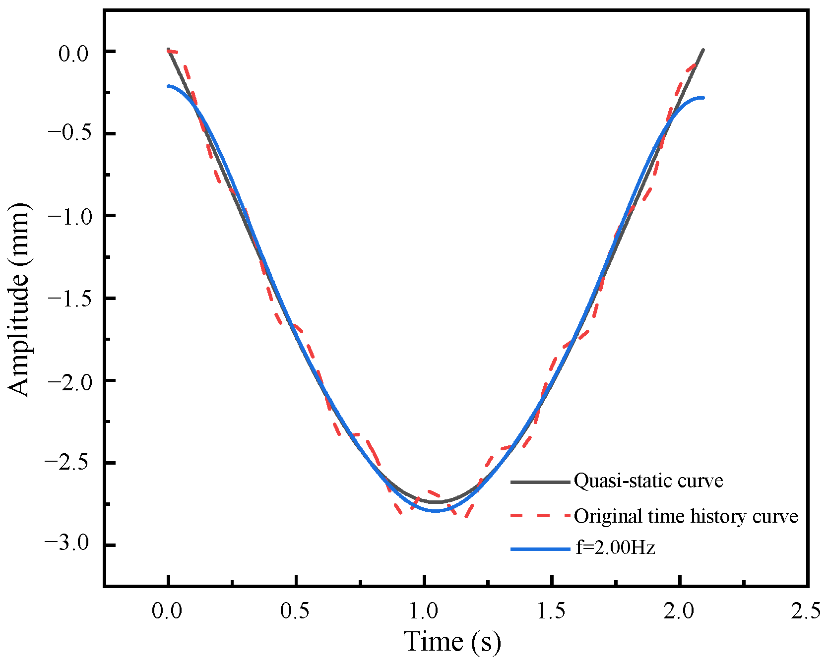
Take the 30-m simply supported T-beam as an example. See Figure 1 and Figure 2 for the section size and superstructure. The vehicle load travels at a uniform speed of 50 km/h, and the midspan time-history curve of the structure is obtained. At the same time, the quasi-static time-history curve of the structure is obtained by driving at a uniform speed of 1 km/h with the same vehicle load, as shown in Figure 8.

In this case, for the quasi-static curve, the statistical characteristic parameters are as follows: the mean is $u_0=-1.65779$, the standard deviation is ${\varpi }_0=0.87003$, the variance is ${\sigma }_0^2=0.75695$, and the absolute maximum is $S_0=2.73974$.

Based on the obtained midspan deflection time-history curve, the re-collected data with different cutoff frequencies $f_1$ are obtained by low-pass filtering, and then the frequency-domain signal is converted into the time-domain signal by inverse Fourier transform, and the results are obtained, as shown in Figure 9.

According to the Nyquist sampling theorem $f_s \ge 2{\mathrm{f}}_{\max }$ [25], the results show that when $f_1=0.7 \mathrm{Hz}$, that is, the acquisition frequency $f_s=1.4 \mathrm{Hz}$, the reconstructed signal is far from the original signal, resulting in mixing phenomenon.

When $f_1=1.5 \mathrm{Hz}$, that is, the acquisition frequency $f_s=3 \mathrm{Hz}$, the reconstructed signal has some deviation from the original signal, but the contour curve is almost the same.

When $f_1=7 \mathrm{Hz}$, that is, when the acquisition frequency $f_s=14 \mathrm{Hz}$, the reconstructed signal is almost the same as the original signal, which is basically consistent.

The above analysis shows that the low-frequency acquisition frequency (1.4 Hz) cannot obtain the complete response of the structure under live load, and the difference is significant, while the high-frequency acquisition frequency (14 Hz) can obtain the relatively complete response of the structure under live load, but the middle sampling frequency (3.0 Hz) is four times lower than the high-frequency acquisition frequency, and the response under live load can still be obtained relatively completely. Therefore, the acquisition frequency of the structural response should not be too low to obtain the structural response; it should not be too high. Although a complete response can be obtained, there is no obvious difference between the results obtained with a relatively low sampling frequency, which increases the difficulty and cost of data processing.

To delve deeper into the concept of reasonable acquisition frequency, it is imperative to employ the fast Fourier transform (FFT) to convert the original time domain signal into a frequency domain signal. This process involves decomposing the signal into a weighted combination of complex exponential functions, thereby establishing a transformational “bridge” between the time domain and the frequency domain. The basic essence of fast Fourier transform is to divide the signal into a certain length, and then carry out a discrete Fourier transform on the signals with two lengths of N/2 and then splice them. Compared with the traditional discrete Fourier transform, the above method saves half the workload [43]. At present, there are two main frequency domain analysis methods: amplitude spectrum analysis and power spectrum analysis. The following will take the midspan deflection signal as an example to explore the advantages and disadvantages of the two analysis methods, and finally determine the estimation method of reasonable acquisition frequency in this paper.

4.2. Estimation Method Based on the Amplitude Spectrum

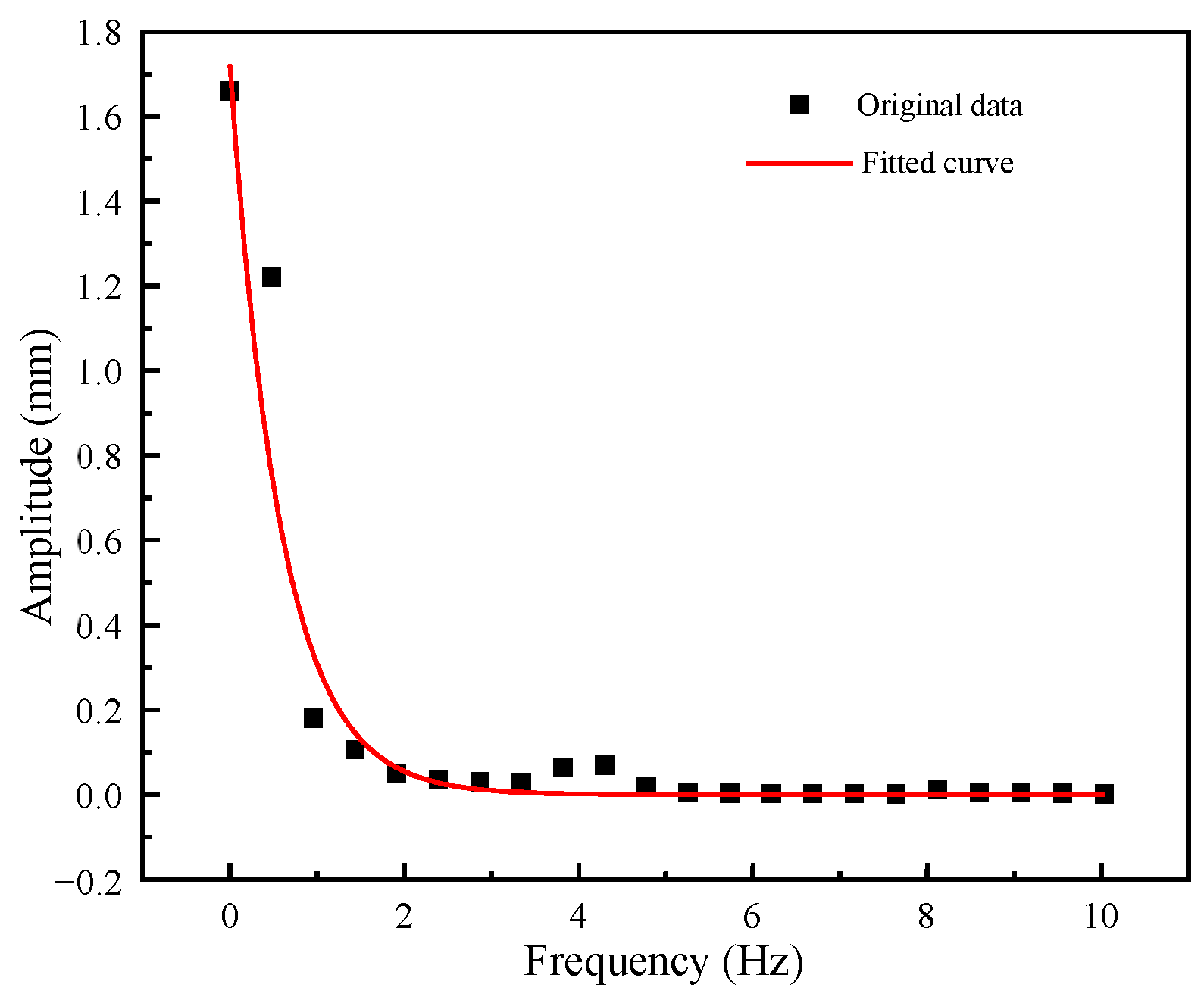
The finite element program is midspan to simulate the probability density function of the amplitude spectrum frequency curve. In conjunction with the original data distribution, it is evident that the distribution pattern of the amplitude of the midspan deflection signal at a given frequency bears resemblance to that of an exponential distribution. The probability density function of the exponential distribution is represented by Formula (7), and the corresponding fitting outcome is depicted in Figure 9.

$$f(x)=\left\{\begin{array}{ll}\frac{1}{\theta }{e}^{-x/\theta },& x>0\\ 0,& else\end{array}\right.$$

(7)

The basic parameter of the probability density function of the exponential distribution shown in Figure 10 is $\theta =0.5817$.

According to the characteristics of the graph, the acquisition frequency is $f =2\mathrm{Hz}$, the high-frequency information is filtered by low-pass filtering, and the frequency-domain signal is converted into the time-domain signal by inverse Fourier transform, as shown in Figure 11.

Statistical analysis of the time-domain-signal-related data obtained after statistical conversion shows that the mean value of the truncated signal deflection time-history curve is $u_1=-1.65968$, the standard deviation is ${\varpi }_1=0.87024$, the variance is ${{\sigma }_1}^2=0.75733$, and the absolute maximum value is $S_1=2.79337$. Compared with the quasi-static data, the error (absolute value) of each digital characteristic is as follows:

Mean relative error:

$${\alpha }_1=\frac{u_0-u_1}{u_0}=\frac{1.65779-1.65968}{1.65779}=0.114\%$$

(8)

Relative error of variance:

$${\delta }_1=\frac{{\sigma }_0^2-{\sigma }_1^2}{{\sigma }_0^2}=\frac{0.75695-0.75733}{0.75695}=0.050\%$$

(9)

Relative error of standard deviation:

$${\psi }_1=\frac{{\varpi }_0-{\varpi }_1}{{\varpi }_0}=\frac{0.87003-0.87024}{0.87003}=0.024\%$$

(10)

Maximum relative error:

$${\mathsf{\Delta }}_1=\frac{S_0-S_1}{S_0}=\frac{2.73976-2.79337}{2.73976}=1.950\%$$

(11)

Because the acquisition frequency is twice the cutoff frequency, i.e., $f_s=2 \mathrm{Hz}$, when the bridge span is 30 m, the vehicle load is about 333 kN, and the vehicle speed is 50 km/h, the reliability calculation of the acquisition frequency of the structure is shown in Formula (12):

$$P\left(f\le f_s\right)=1-e^{-\frac{x}{\theta }}=96.790\%$$

(12)

The meaning of the above formula is to determine the ratio of the area of the amplitude spectrum at the cutoff frequency of 2 Hz to the area of the original amplitude spectrum function. Similarly, when the acquisition frequencies are 2 Hz, 2.5 Hz, 3.0 Hz, and 3.25 Hz, the reliability of the acquisition frequency and the error of the truncated time-history curve are respectively selected, and the results are summarized as shown in

Table 4. Digital Characteristics and Reliability Analysis Based on Amplitude Spectrum.

Sampling Frequency (Hz)	${\mathit{\sigma }}_1^2$	${\mathit{\sigma }}_0^2$	$\mathit{\delta }$	${\mathit{\varpi }}_1$	${\mathit{\varpi }}_0$	$\mathit{\psi }$	${\mathit{S}}_1$	${\mathit{S}}_0$	$\mathsf{\Delta }$	Pr (%)
2.00	0.746	0.756	1.39	0.863	0.870	0.70	2.881	2.740	5.16	96.79
2.50	0.746	0.756	1.40	0.863	0.870	0.70	2.881	2.740	5.15	98.64
3.00	0.752	0.756	0.64	0.867	0.870	0.32	2.774	2.740	1.24	99.42
3.25	0.754	0.756	0.35	0.868	0.870	0.17	2.754	2.740	0.54	99.75
4.00	0.757	0.756	0.05	0.870	0.870	0.02	2.793	2.740	1.96	99.89

.

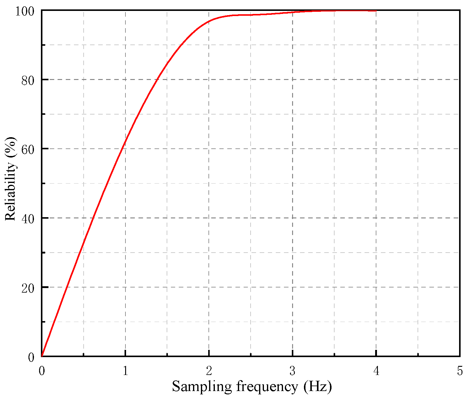
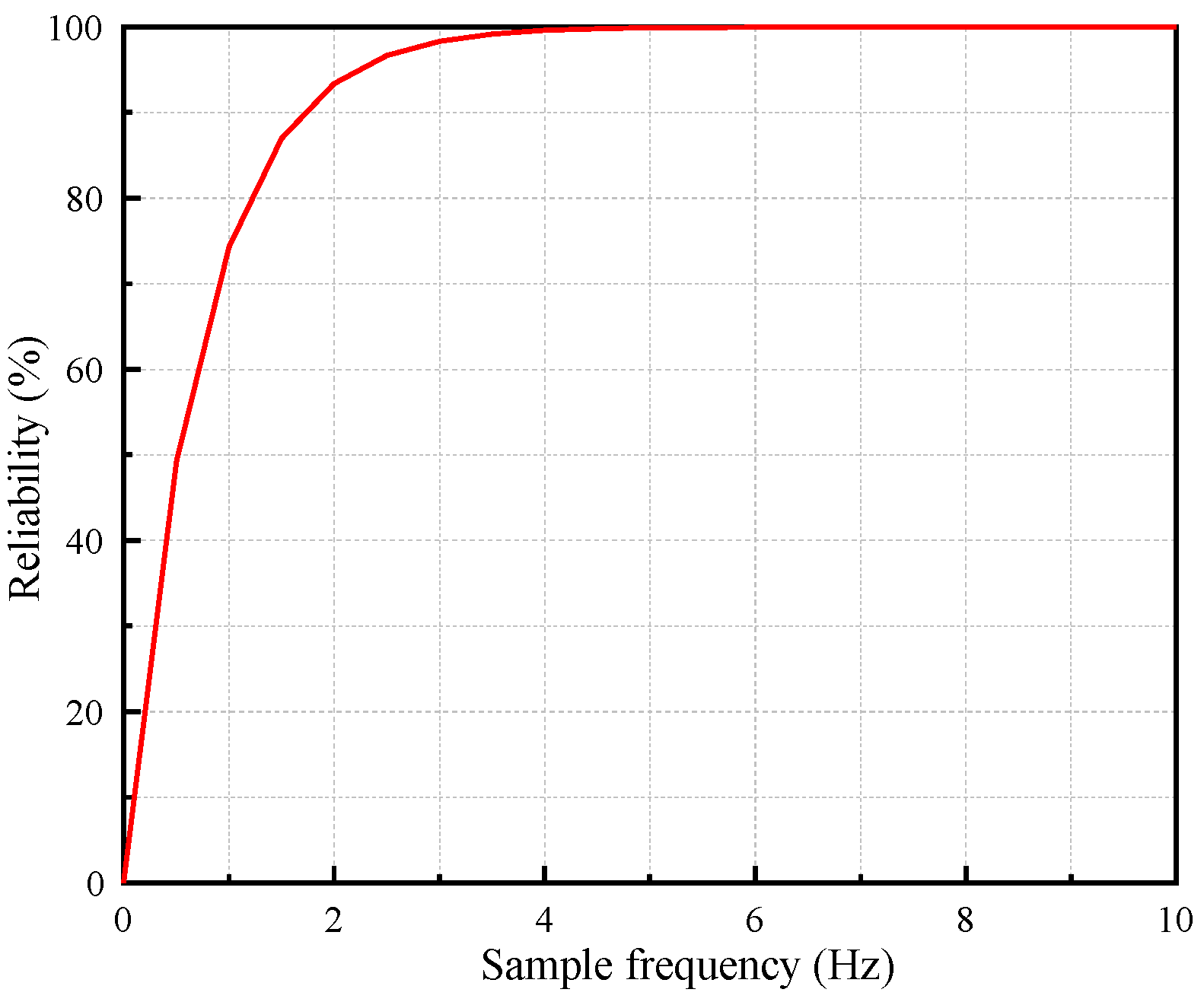
Draw the distribution diagram of the cumulative function of structural acquisition frequency reliability under this working condition, as shown in Figure 12.

When the cutoff frequency is $f_1=1.0 \mathrm{Hz}$ and the acquisition frequency is $f_{1 }=2.0 \mathrm{Hz}$, the error of each digital characteristic of the signal is close to or less than 5%, and the reliability of the acquisition frequency is greater than 95%, which shows that it meets the requirements of practical engineering.

4.3. Estimation Method Based on the Power Spectrum

The selection method for the cutoff frequency depends on the spectrogram. Once the spectrogram is distorted or too complicated, it is difficult to find the accurate cutoff frequency [44]. Therefore, refer to the definition of the cutoff frequency in the sensor [45]: when the amplitude of the input signal is kept constant, the output signal is reduced to 0.707 times the maximum value by changing the frequency, which is expressed by frequency response characteristics; that is, the cutoff frequency is at the point of −3 dB.

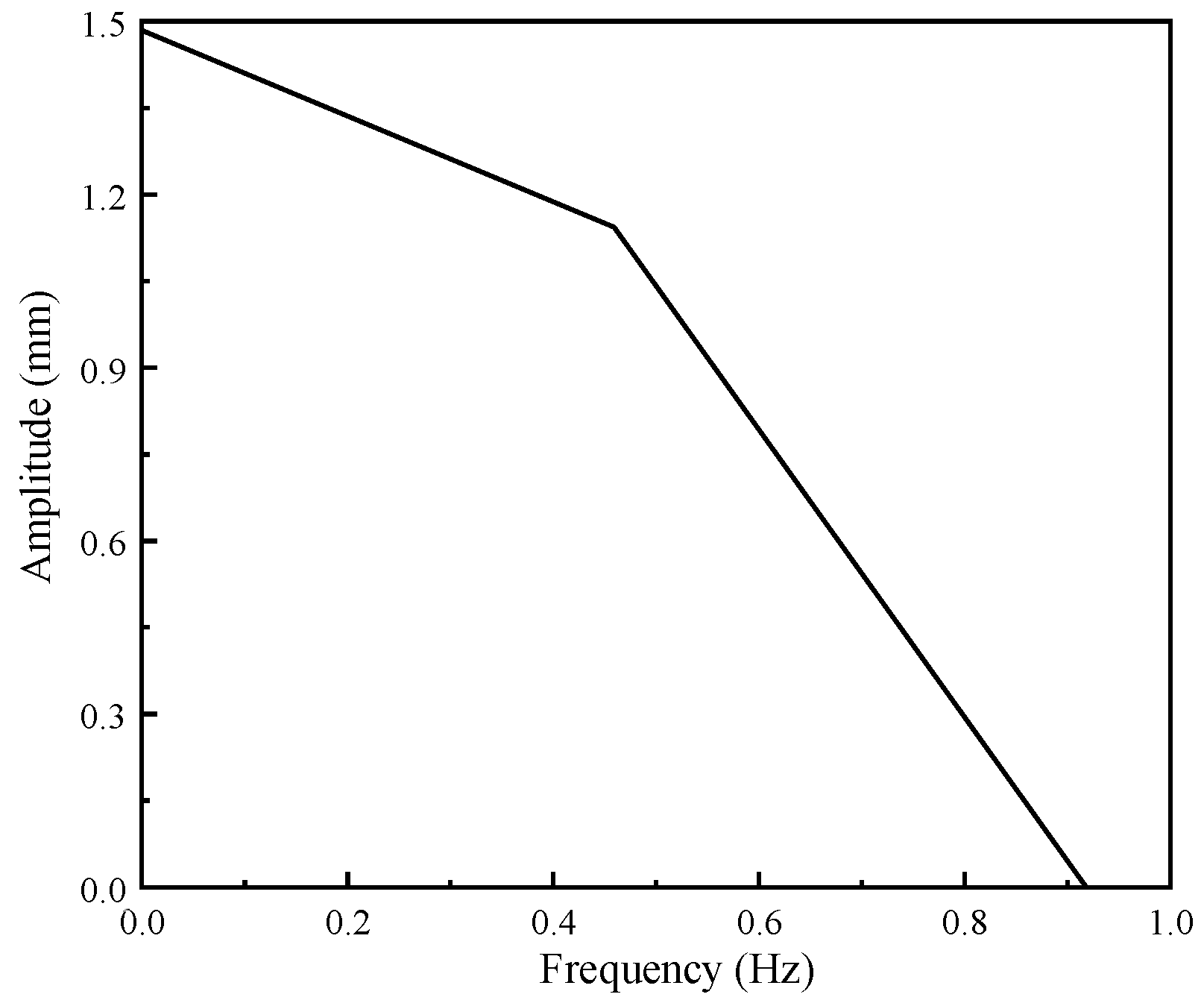
The power spectral density of the signal describes the distribution of the power-limited signal with the frequency in the frequency domain. In order to highlight the main frequency components, the frequency at the −3 dB point of the energy power spectrum function is selected as the cutoff frequency, and the amplitude spectrum corresponding to this frequency is about 0.707 times the maximum value; that is, the cutoff frequency $f_1=0.62 \mathrm{Hz}$ and the acquisition frequency $f_s=1.24 \mathrm{Hz}$, as shown in Figure 13.

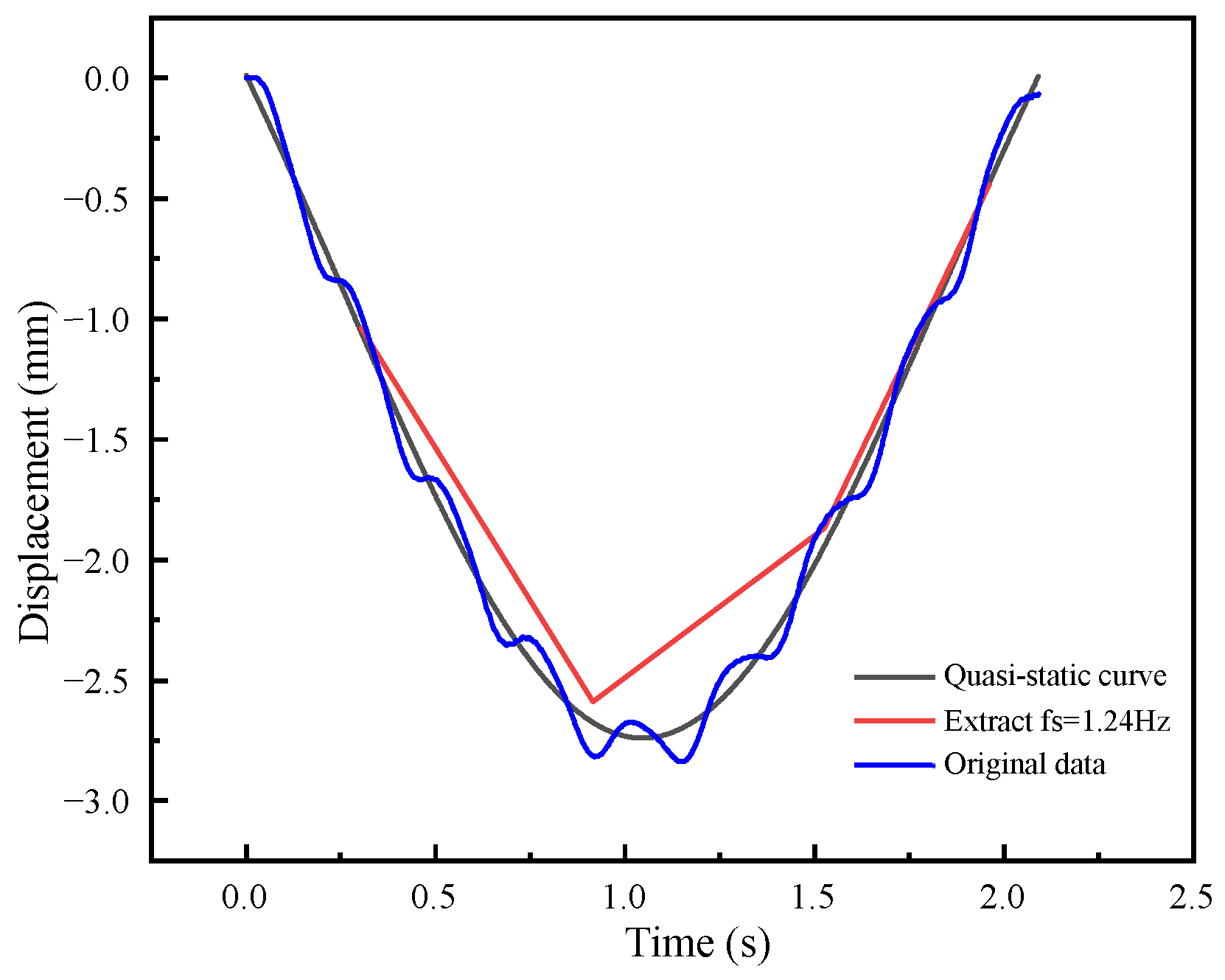
The high-frequency components are removed by low-pass filtering, and the frequency-domain signal is converted into the time-domain signal and compared with the quasi-static curve, as shown in Figure 14.

Through the statistical calculation of the discrete data of time domain signals, it is found that the signal with a truncated signal of $f_1=0.62 \mathrm{Hz}$ has a mean value of $u_1=-1.65968$, a standard deviation of ${\varpi }_1= 0.86385$, a variance of ${\sigma }_1^{2 }= 0.74623$, and an absolute maximum value of $S_1=2.88$.

For this 30-m span simply supported beam bridge, the first-order natural frequency is 4.3019 Hz, the second-order natural frequency is 8.9381 Hz, and the third-order natural frequency is 13.061 Hz. The disturbance frequency ${\varpi }_1=1\times \mathsf{\pi } \times \mathsf{\upsilon }/l=1.454\mathrm{Hz}$ of the moving force, the cutoff frequency of the midspan deflection signal is $f_1=0.62 \mathrm{Hz}$, and the acquisition frequency $f_s=1.24 \mathrm{Hz}$, which is slightly less than the disturbance frequency of the first-order moving force. The error (absolute value) of the cutoff frequency reconstruction curve and various digital characteristics is as follows:

Mean relative error:

$${\alpha }_1=\frac{u_0-u_1}{u_0}=\frac{1.65779-1.65968}{1.65779}=0.114\%$$

(13)

Relative error of variance:

$${\delta }_1=\frac{{\sigma }_0^2-{\sigma }_1^2}{{\sigma }_0^2}=\frac{0.75695-0.74623}{0.75695}=1.416\%$$

(14)

Relative error of standard deviation:

$${\psi }_1=\frac{{\varpi }_0-{\varpi }_1}{{\varpi }_0}=\frac{0.87003-0.86385}{0.87003}=0.710\%$$

(15)

Maximum relative error:

$${\mathsf{\Delta }}_1=\frac{S_0-S_1}{S_0}=\frac{2.73976-2.8810}{2.73976}=5.150\%$$

(16)

Because the acquisition frequency is twice the cutoff frequency, i.e., $f_s=1.24 \mathrm{Hz}$, when the bridge span is 30 m, the vehicle load is about 333 kN, and the vehicle speed is 50 km/h, the reliability calculation of the acquisition frequency of the structure is shown in Formula (17):

$$P\left(f\le f_s\right)=1-e^{-\frac{x}{\theta }}=95.860\%$$

(17)

The meaning of the above formula is to determine the ratio of the amplitude spectrum area under the acquisition frequency of 1.24 Hz to the area of the original amplitude spectrum function. Draw the cumulative function distribution diagram of the structural acquisition frequency reliability under this working condition, as shown in Figure 15.

When the cutoff frequency $f_1=0.62 \mathrm{Hz}$ and the acquisition frequency $f_s=1.24 \mathrm{Hz}$, the error of each digital characteristic of the signal is close to or less than 5%, and the reliability of the acquisition frequency is more than 95%, which shows that it meets the requirements of practical engineering.

4.4. Determination of the Acquisition Frequency Estimation Method

Accurate selection of the appropriate cutoff frequency is a fundamental aspect within the extended discretization of structural response signals and analytical mode decomposition (AMD). Currently, the procedure for determining the cutoff frequency involves performing a Fourier transform on the original time series to obtain its spectrum. Subsequently, a position is identified between two poles in the spectrum, and the frequency value corresponding to this position is considered as the selected cutoff frequency [9].

The estimation of the acquisition frequency may be subject to subjective influences when exclusively depending on the amplitude spectrum. The selection of a certain cutoff frequency is crucial, since it should be determined in accordance with the distribution features of the probability density function. In order to attain a signal curve reconstruction reliability of approximately 95%, it is necessary to conduct experiments with different cutoff frequencies, utilizing the structural acquisition frequency. The accuracy of determining the cutoff frequency can be achieved through power spectrum estimation. However, it is observed that the fitting error of the power spectrum probability density function is higher compared to that of the amplitude spectrum probability density function. This discrepancy significantly impacts the reliability calculation of the acquisition frequency.

Based on the aforementioned information, the following notions are proposed: This study has two primary objectives. Our primary objective is to ascertain the cutoff frequency of the signal by an analysis of the amplitude-frequency curve of the power spectrum. Additionally, our objective is to determine the probability density function of the initial time-history curve data by utilizing the amplitude spectrum. Furthermore, we will compute the digital characteristic errors for both the low-pass signal with a cutoff frequency and the quasi-static signal. The paper demonstrates the reliability of the suggested method by measuring the ratio between the amplitude spectrum area of the acquired signal at an appropriate acquisition frequency and the area of the amplitude spectrum function of the original signal.

5. Reliability Verification of the Frequency Estimation Value of Midspan Deflection Acquisition

Based on the error caused by the exponential distribution function simulation and the reliability probability integration method, it is necessary to further verify the calculation results of the bridge structure’s acquisition frequency reliability under the above working conditions.

For the midspan deflection time-history curve, the correctness of the reliability calculation results with a cutoff frequency of $f_1=0.62 \mathrm{Hz}$ and an acquisition frequency of $f_s=1.24 \mathrm{Hz}$ is verified.

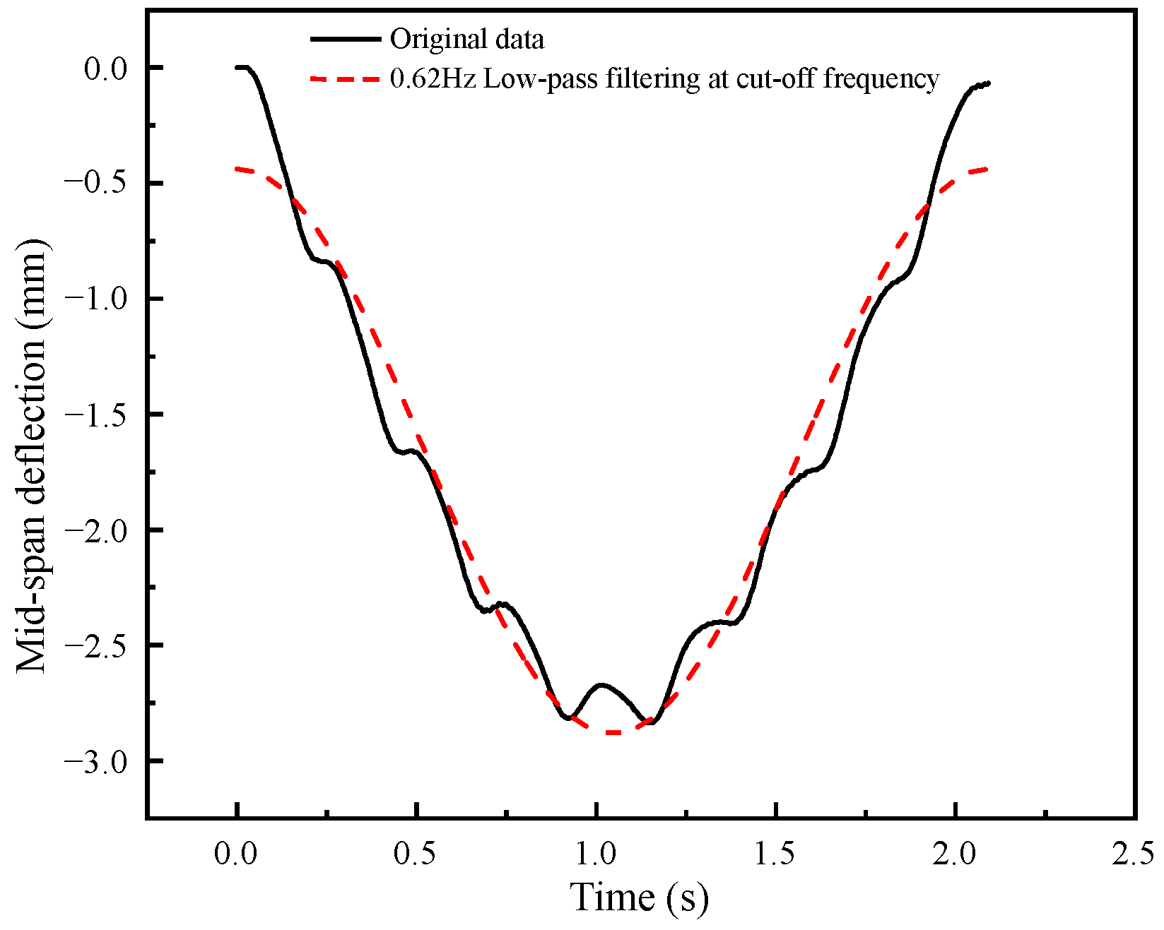
The signal acquisition interval $\mathsf{\Delta }t =0.00115 \mathrm{s}$ of the bridge simulation analysis is 869 Hz. Now, the acquisition frequency is changed to 1.24 Hz, which is equivalent to reducing every 603 items of data in the original signal to one item of data, and then forming a new original signal. Through Fourier transform, the time domain signal is converted into the frequency domain signal, and the amplitude spectrum curve of the frequency domain signal is obtained, as shown in Figure 16.

When the acquisition frequency is 1.24 Hz, the cutoff frequency of the signal is 0.62 Hz, the mean value of the amplitude spectrum function is $u_1=-1.4582$, the standard deviation is ${\varpi }_1=0.94032$, the variance is ${{\sigma }_1}^2=0.88421$, and the absolute maximum value is $S_1=2.5895$. Compared with the quasi-static data, the error (absolute value) of each digital characteristic is as follows:

Mean relative error:

$${\alpha }_1=\frac{u_0-u_1}{u_0}=\frac{1.65779-1.4852}{1.65779}=10.410\%$$

(18)

Relative error of variance:

$${\delta }_1=\frac{{\sigma }_0^2-{\sigma }_1^2}{{\sigma }_0^2}=\frac{0.75695-0.88421}{0.75695}=16.812\%$$

(19)

Relative error of standard deviation:

$${\psi }_1=\frac{{\varpi }_0-{\varpi }_1}{{\varpi }_0}=\frac{0.87003-0.94032}{0.87003}=8.079\%$$

(20)

Maximum relative error:

$${\mathsf{\Delta }}_1=\frac{S_0-S_1}{S_0}=\frac{2.73976-2.5895}{2.73976}=5.484\%$$

(21)

The reliability of acquisition frequency is calculated as follows:

$$P_r=P\left(f<1.24 \mathrm{Hz}\right)=\frac{A_1}{A_0}=\frac{{\sum }_{i=1}^n{g}_1\left(x_i\right)f_i}{{\sum }_{i=1}^{n}g\left(x_i\right)f_i}=\frac{0.86423}{0.94038}=91.900\%$$

(22)

where, $g_1\left(x\right)$ is the amplitude spectrum simulation function of the quasi-static curve of the original signal; $g\left(x\right)$ is the extracted amplitude spectrum function simulated with a frequency of 1.24 Hz; $A_1$ is the area of the amplitude spectrum function at a sampling frequency of 1.24 Hz; $A_0$ is the area of the original amplitude spectrum function at a acquisition frequency of 869 Hz.

As can be seen from Figure 17, when the acquisition frequency is 1.24 Hz, the digital characteristics of the midspan deflection signal of the bridge are relatively consistent with the quasi-static curve, and the change is relatively small, which shows that the reasonable acquisition frequency analysis method of the midspan deflection proposed in this paper is feasible.

6. Conclusions

The present study utilizes the principles of reliability theory to analyze the frequency domain characteristics of the vehicle-bridge coupling system. The primary focus of this study centers on the analysis of the time-history curve pertaining to the deflection response of the midspan. The aim of this study is to determine the optimal frequency of acquisition for the given structure. This study aims to analyze the maximum error in response and verify the reliability of the calculation results for the acquisition frequency. This is carried out by examining the simulation error of the exponential distribution function and the integration method for reliability probability. The analysis can be concisely summarized as follows:

(1)

This paper presents an introduction to the ideas of sensor acquisition frequency and appropriate acquisition frequency, utilizing the evaluation method of live loading and the fundamental principles of reliability. An evaluation of the reliability of the vehicle-bridge connection system is conducted through the utilization of the probability integration approach. To examine the system’s response in the frequency domain, the time-history curve of the midspan deflection response is employed. It is discovered that the power spectrum at a level of −3 dB corresponds to the frequency at which the response is cut off. The determined cutoff frequency is observed to be twice the acceptable acquisition frequency.

(2)

Based on the definition of a quasi-static response, it can be deduced that the velocity of a load does not exert any influence on the quasi-static response of a bridge structure. Therefore, this paper presents the derivation of bridge deflection components and quasi-static response, as well as the recommended approach for finite element extraction. The GUESS curve is utilized to model the time-history curve of midspan deflection.

(3)

This study centers on examining the frequency features of deflection in the midspan section of a beam bridge that is supported in a basic manner. This study presents a novel approach for finding the cutoff frequency of the structural response by considering the unique characteristics of amplitude spectrum estimation and power spectrum estimation in frequency domain analysis. This methodology entails utilizing the amplitude-frequency curve of the power spectrum to determine the cutoff frequency of the signal. The estimation of the probability density function of the original time-history curve data is then conducted using the amplitude spectrum. The digital characteristic errors of the previously specified low-pass signal with a cutoff frequency and the quasi-static signal are calculated. The verification of the suggested method for acquiring midspan deflection is conducted by examining the ratio between the area of the amplitude spectrum of the acquired signal at an appropriate acquisition frequency and the area of the amplitude spectrum function of the original signal.

In this study, the empirical formula for determining the appropriate acquisition frequency of midspan section deflection in a simply supported T-beam bridge construction is derived using correlation analysis and multiple linear regression. The validity of this formula is then confirmed by experimentation using a laboratory vehicle-bridge coupling model. Ultimately, this concept is further expanded upon to encompass the practical implementation of a real-time bridge health monitoring system.