Reconstruction Algorithm Optimization Based on Multi-Iteration Adaptive Regularity for Laser Absorption Spectroscopy Tomography

Abstract

Laser absorption spectroscopy tomography is an effective combustion diagnostic method for obtaining simultaneous two-dimensional distribution measurements of temperature and gas molar concentrations. For the reconstruction process of complex combustion flames, a new algorithm named ‘multi-iterative adaptive optimization regularization’ (MIARO) is proposed. This algorithm is a further development of another algorithm known as the ‘modified adaptive algebraic reconstruction technique’ (MAART) with the improvement of the initial value and adaptive regularization parameter selections. In MIARO, the problem of the MAART’s initial value sensitivity is compensated for, and in addition, reconstruction parameters are also introduced into the regularization so that both the quality of reconstruction and the convergence of regularization are guaranteed. In butane burner experiments, an average relative error of 1.82% was achieved with MIARO, compared to 2.44% with MAART, which is a significant reduction of 25.1%. The simulation and experimental results clearly demonstrate that the MIARO algorithm can be used to reconstruct dynamic combustion fields and eliminate boundary artifacts with improved measurement accuracy and robustness.

1. Introduction

The diagnosis of combustion processes is a vital tool for both scientific research and industrial applications. Over the years, various techniques have been devised and implemented for this purpose. Acoustic thermometry (AT) [1,2,3,4], coherent anti-Stokes Raman scattering spectrometry (CARS) [5], planar laser-induced fluorescence (PLIF) [6], radiation thermometry [7,8] and laser absorption spectroscopy (LAS) are examples of such techniques [9,10]. As a typical non-contact measurement method, tunable diode laser absorption spectroscopy (TDLAS) has many advantages, such as a fast measurement response, high accuracy, high sensitivity, the simultaneous measurement of multiple parameters, etc. TDLAS has been widely used in combustion diagnostics and trace-gas detection, and its performance is particularly demonstrated when multiple-parameter measurement is required. A more recent development in this field is the tunable diode laser absorption tomography (TDLAT) technique [11,12], which combines the TDLAS technique and the computed tomography (CT) technique. TDLAT has been gradually developed and has been widely applied [13]. By detecting the spectral data for multiple angles and laser paths through the measured field, combined with image reconstruction algorithms, the visualization of temperature and component concentration distributions in complex combustion fields is achieved using TDLAT, which was used in the experiments in this research [14,15].

Two-dimensional distribution reconstruction is essentially the process of solving the physical properties of each reconstruction parameter of a target region based on the measured projection values and sensitivity matrix of a measurement system. Reconstruction algorithms play a key role as a bridge between the physical parameters and measured projection values. Algebraic iterative-type reconstruction algorithms allow for the incorporation of a priori knowledge about the target field into the iterative process, and they are widely used in incomplete data reconstruction. However, the reconstruction process itself is an inverse problem that is often ill posed. In order to solve this type of ill-posed problem, it is usually necessary to regularize the constraints on the reconstructed and true distributions with the aid of additional a priori information to suppress the noise and artifacts introduced by data incompleteness and to effectively improve the instability of the inverse problem of process tomography. Therefore, the establishment of suitable and accurate regularization terms becomes key to the success of a regularization method. Li et al. [16] developed a Modified Adaptive Algebraic Reconstruction Technique (MAART) to reconstruct the distributions of concentration and temperature simultaneously under incomplete projections for fast computation and high quality. In this method, the author introduced two correction coefficients, the relaxation factor and the smoothing factor, on the basis of the traditional algebraic reconstruction algorithm. Through numerical simulations, the influence of the correction coefficients on the convergence of the algorithm and the imaging accuracy were analyzed, and the value interval of the correction coefficients was optimized [17,18].

In this paper, a new reconstruction algorithm, named the Multi-iterative Adaptive Regular Optimization (MIARO) algorithm, is proposed, which is a further development of MAART, and the initial value and adaptive regularization parameter selections are its main added features. This proposed algorithm solves the problem of the initial value sensitivity encountered in MAART by adopting multiple iterations and by introducing reconstruction parameters into the regularization parameters to determine the adaptive iteration step size and establish a regularization optimization control process, so that the global optimal solution can be found in a shorter time, and therefore, both the quality of the reconstruction objective and the convergence of the regularization can be guaranteed.

2. Principle of Tomographic Laser Absorption

2.1. Laser Absorption Spectroscopy Tomography

Laser absorption spectroscopy (LAS) is a method of image reconstruction that works by inverting multiple line-of-sight (LOS) measurements to obtain the two-dimensional distribution of parameters in a region of interest (ROI) [19,20]. According to the Beer–Lambert law, the spectral absorptivity α(v) in a gaseous medium along the path l (cm) at the frequency ν (cm⁻¹) can be expressed as [21,22]

$$\alpha \left(v\right)=-\ln (\frac{I_{\mathrm{t}}}{I_0})={\displaystyle {\int }_0^{L}P\left(l\right)X\left(l\right)S_v(T(l))\phi (v,l)dl}$$

(1)

where I₀ and I_t are the incident and transmitted laser intensities, l is the position along the total length of the path L (cm), P(l) (atm) is the total pressure, X(l) is the gas mole fraction, T(l) (K) is the gas temperature, S(T) (cm⁻² atm⁻¹) is the temperature-dependent line intensity, and φ(v) (cm⁻¹) is the linear function. Since the linear function is normalized to ${\int }_{-\infty }^{+\infty }$φ(v, l)dv ≡ 1, the absorbing area along the path can be expressed as

$$A_{v,i}={\displaystyle {\int }_{-\infty }^{\infty }{\alpha }_v}dv={\displaystyle {\int }_0^{L}P\left(l\right)X\left(l\right)S_v(T(l))dl}={\displaystyle {\int }_0^L{\alpha }_{v}dl}$$

(2)

where v is the wavenumber. α_v is the path integral density, also known as the local integral absorption area.

For absorption spectroscopy tomography, Equation (2) can be rewritten in the following matrix form to improve computational efficiency:

$$\mathit{L}{\mathsf{\alpha }}_v={\mathit{A}}_v$$

(3)

where L ∈ ℝ^M×N is the sensitivity matrix, which is calculated based on the geometrical distribution of the laser prior to the measurement. Its element l_i,j represents the laser path of the i-th laser beam when it passes through the j-th pixel. i (i = 1, 2...., M) and j (j = 1, 2..., N) are the indexes of the laser beam and pixel, respectively. The spectrally integrated absorption area A_v = {A_v,1, A_v,2, A_v,N }^T and the locally integrated absorption area α_v = {α_v,1, α_v,2, α_v,N }^T are column vectors, where α_v,j = P_j X_j S(T_j), from which the distribution of flame temperature and gas concentration parameters can be extracted [23,24,25].

2.2. Principles of the MIARO Algorithm

Using the proposed algorithm MIARO, the global optimal solution can be found in a shorter time because of the realization of the adaptive iteration step size and the regular optimization of process control, which takes advantage of different iteration algorithms. Firstly, global optimization is sought by the Landweber algorithm, and the initial iteration value is provided based on MAART by iterating a small number of times. The Landweber algorithm is a synchronous iterative reconstruction algorithm or simultaneous iterative reconstruction technique (SIRT), where each iteration involves all rows of the system of equations, which can realize fast global optimization. The specific iteration form is

$${\mathsf{\alpha }}^{(k+1)}={\mathsf{\alpha }}^{(k)}-{\lambda }_k{\mathit{L}}^T\left(\mathit{L}{\mathsf{\alpha }}^{(k)}-\mathit{A}\right)$$

(4)

where α is the reconstruction parameter, and A is the integral projection value. L is the sensitivity matrix, and λ_k is the k-th iteration step. The specific value of λ_k can be found in refs. [26,27], and its expression is as follows:

$${\lambda }_k=\frac{〈{\mathit{r}}^{(k)},{\mathit{r}}^{(k)}〉}{{‖{\mathit{L}}^T{\mathit{r}}^{(k)}‖}_2^2},{\mathit{r}}^{(k)}=\mathit{A}-\mathit{L}{\mathsf{\alpha }}^{(k)}$$

(5)

where <, > denotes the inner product.

In MAART, the adaptive change in the iterative step can be implemented, and reconstruction parameters can be introduced into the iterative relationship. The higher the contribution of a reconstruction parameter to a projection value, the larger the possible step size of an iteration. But the MAART iterative algorithm is sensitive to the initial value, and it cannot be set to 0. The initial parameter is provided via a global search of optimization using the Landweber algorithm so as to realize a faster iterative convergence. The iterative form of the MAART algorithm is expressed as [28]

$${\alpha }^{(k+1,i)}={\alpha }^{(k,i)}-\lambda \left(L_i{\alpha }^{(k,i)}-A_i\right)$$

(6)

$$\lambda =\beta \times \frac{{\alpha }_j^{(k)}{L}_{ij}}{{\displaystyle \sum _{j=1}^N{\alpha }_j^{(k)}{L}_{ij}}}$$

(7)

The reconstruction process is often a kind of pathological or ill-posed inverse problem. In order to solve such a problem, it is necessary to regularize the constraints on the reconstructed and true distributions with the aid of some additional a priori information to suppress the noise and artifacts introduced by data incompleteness. Regularization can effectively improve the instability of the laminar inverse problem. Therefore, the establishment of suitable and accurate regularization terms is key to the success of a regularization method. One of the frequently adopted regularization models is Tikhonov regularization, which is usually used to attenuate the smoothness of the mutation response of neighboring points in a reconstruction region, and a typical function is defined as follows:

$${\alpha }_{(i,j)}^{\left(k\right)}=(1-\theta ){\alpha }_{(i,j)}^{\left(k-1\right)}+\theta ({\displaystyle \sum _{y=j-1}^{j+1}{\displaystyle \sum _{x=i-1}^{i+1}{\alpha }_{(x,y)}^{\left(k-1\right)}}})/8$$

(8)

where i, j is the rank order of a grid. The Adaptive Regular Optimization (ARO) algorithm proposed here is used to realize the change in the adaptive regularization parameters and to introduce the reconstruction parameters into the iterative process. In ARO, the traditional fixed smoothing coefficient θ cannot accurately reflect the actual distribution characteristics, and the specific choice of the smoothing slip coefficient will also be directly related to the reconstruction quality. When θ takes a larger value, the reconstruction parameters will be over-smoothed. On the other hand, a smaller value of θ can result in the reconstruction parameters falling into a local optimal solution, and hence, the reconstructed distribution tends to become steeper. Therefore, in the iteration process, θ needs to be adjusted according to the trend of the reconstruction parameters, and the amplitude of the smoothing coefficient θ can be automatically tuned according to the ratio of the reconstruction parameter to the mean value of other reconstruction parameters around it [29]. This ensures both the quality of the reconstructed target and the convergence of regularization. The specific mathematical expression is as follows:

$$\theta =\gamma \frac{({\displaystyle \sum _{y=j-1}^{j+1}{\displaystyle \sum _{x=i-1}^{i+1}{\alpha }_{(x,y)}^{\left(k-1\right)}}})}{{\alpha }_{ARO}^{(k-1)}}$$

(9)

where γ is the initial regularization parameter, which is taken as 0.8 in this research.

A termination condition based on the relative difference in the projected values is also proposed in ARO. The iteration terminates when the relative difference in the phase’s projected value reaches the threshold ε, where $\kappa \le \epsilon$. Equation (10) is used to specifically define $\kappa .$

$$\kappa =\frac{\left|L{\alpha }_{ARO}^{\left(k\right)}-A\right|}{\left|A\right|}$$

(10)

where the index k is the number of iterations, and ${\alpha }_{ARO}^0$ is the initial reconstruction value. In this application, a threshold of 0.001 was used. The detailed steps of the algorithm are shown in

Table 1. Steps for implementing the multi-iterative adaptive optimization algorithm.

Serial Number	Specific Realization Steps
1	Obtain the initialized reconstruction parameters α0 =αLandweber using the Landweber algorithm;
2	Establish the image αiter by applying the MAART algorithm;
3	Impose the nonnegativity constraint such that all negative elements of α in the reconstruction process are set to 0, yielding the new reconstruction parameter α;
4	Examine whether the convergence condition ($a_{iter}^{(k+1)}$ − $a_{iter}^{\left(k\right)}$)/$a_{iter}^{\left(k\right)}$ ≤ ε is satisfied. If the condition is satisfied, directly execute step 6; otherwise, go to step 5.
5	Enter the adaptive optimization algorithm: Execute Equations (8) and (9) to iterate the process so as to update the regularization parameter θ; When the ratio κ satisfies κ ≤ ε in Equation (10), then set $a_{iter}^{(k+1)}$ = $a_{ARO}^{\left(k\right)}$, end the iteration process, and return to step 2 for the next generation step; When the convergence condition is not met, revert to the regularization optimization process;
6	Withdraw from the program.

.

The iterative reconstruction algorithm based on the multi-iterative adaptive optimization algorithm can achieve better quality for reconstructed images and can reduce the requirements for iteration parameters. The specific algorithm flowchart is shown in Figure 1 below:

3. Simulated Results and Error Analysis

3.1. Reconstructed Distribution Setup for Dynamic Temperature Field Simulation

In hydrocarbon flames, water vapor, the main product of the combustion process, absorbs strongly in the near-infrared region. Therefore, water vapor was chosen as the target absorbing species in both simulations and experiments. Two absorption spectra, centered at v₁ = 7185.6 cm⁻¹ and v₂ = 7444.36 cm⁻¹, were used in this work because of their moderate line intensities and good temperature sensitivity. The specific parameters of the two chosen spectral lines can be combined with the HITRAN database [30]. The absorbances of the two spectral lines at different temperatures are given in Figure 2a,b, and the line intensities and intensity ratio of the two spectral lines are depicted in Figure 2c.

According to some classical combustion field parameter data, in an adducted combustion chamber, the temperature T is in the range of 600~1600 K, and the concentration X is between 0.02 and 0.05 mol/mol. In order to verify the validity of the proposed method, two regions with non-uniform temperature and H₂O concentration distributions were chosen to simulate the complex combustion field distributions. Figure 3 shows the axisymmetric and non-axisymmetric distributions used for simulations. The axisymmetric distributions for both water vapor and temperature are Gaussian. The non-uniform regions were created using one symmetric and three overlaid asymmetric Gaussian distributions. The scanning area for reconstruction was 200 mm × 200 mm, with a grid division of 120 × 120 and a grid size of 1.67 mm × 1.67 mm. The specific field distributions are expressed using Equations (11) and (12):

$$T=600+{\displaystyle \sum _{k=1}^{K}1600\cdot {\eta }^k\cdot \exp \left[-\frac{{\left(x-x_c^k\right)}^2+{\left(y-y_c^k\right)}^2}{{\sigma }^2}\right]}$$

(11)

$$X=0.02+{\displaystyle \sum _{k=1}^{K}0.05\cdot {\eta }^k\cdot \exp \left[-\frac{{\left(x-x_c^k\right)}^2+{\left(y-y_c^k\right)}^2}{{\sigma }^2}\right]}$$

(12)

where x and y denote the horizontal and vertical coordinates of the reconstructed region, respectively. (x_c^k, y_c^k) is the center of the k-th Gaussian peak, η is the Gaussian distribution peak parameter, and σ is the standard deviation. The detailed distribution parameters used for the simulations are provided in

Table 2. Axisymmetric and non-axisymmetric distribution settings.

	η	(${\mathit{x}}_{\mathit{k}}^{\mathit{c}}$, ${\mathit{y}}_{\mathit{k}}^{\mathit{c}}$) (cm)	σ (cm)
Axisymmetric simulation distribution	0.4	(10, 10)	4
Non-axisymmetric simulation distribution	0.4	(6, 14)	4
	0.35	(14, 14)
	0.2	(9, 6)

.

Often, in complex combustion flame parameter tests, the acquired signals are inevitably affected by mechanical vibrations and thermal radiation in the flame. Photodetectors are also subjected to calibration errors. In order to evaluate the performance of the system in noisy environments, 2%, 4%, 6% and 8% uniform noise levels were added to the LOS measurements A to study and analyze the stability of the MIARO algorithm in complex combustion field reconstruction applications [31,32].

3.2. Reconstruction Error Comparison Principle

In this paper, the average relative error (ARE) and average root-mean-square error (ARMSE) are used to evaluate the quality of the temperature and concentration field reconstruction. The specific mathematical formulae are expressed using Equations (13) and (14) [33,34].

$$\mathrm{ARE}=\frac{1}{n}{\displaystyle {\sum }_{r=1}^n(\frac{1}{N}{\displaystyle {\sum }_{j=1}^N\left|\frac{x_{rec,j}-x_{sim,j}}{x_{sim,j}}\right|})}$$

(13)

$$\mathrm{ARMSE}=\frac{1}{n}{\displaystyle {\sum }_{r=1}^n(\sqrt{{\displaystyle {\sum }_{i=1}^N{(x_{rec,j}-x_{sim,j})}^2}}/\sqrt{{\displaystyle {\sum }_{i=1}^N{(x_{sim,j})}^2}})}$$

(14)

where n is the number of simulations conducted per group, and N is the number of reconstruction parameters to be solved. x_rec,i and x_sim,i denote the reconstruction value and the true value (temperature or concentration), respectively. In the simulation, n was 100.

3.3. Discussion and Analysis of Reconstruction Simulation Results

The proposed MIARO algorithm was validated using both the axisymmetric and non-axisymmetric numerical models via simulation. In order to verify its superiority, MIARO was compared with ART, Landweber and MAART, three classical iterative reconstruction algorithms in terms of accuracy and robustness.

3.3.1. Axisymmetric Simulation Distribution

Using the above-mentioned four algorithms, simulations were conducted to reconstruct axisymmetrically distributed temperature and vapor concentration fields. Figure 4 shows the reconstruction results. It can be seen that there are no notable differences between ART, Landweber and MAART. In fact, the Landweber algorithm presents the largest error at the edge. In contrast, the reconstruction error and the fluctuation at the edge achieved using the MIARO algorithm are significantly reduced, which clearly demonstrates the superiority of MIARO.

Further analyses were conducted on the reconstruction results at the symmetric peak centers over various cross-sections. The reconstruction results over a typical cross-section are presented in Figure 5. It can be found that the reconstruction errors at the peak with the MIARO algorithm for both temperature and concentration are much smaller. The maximum error of temperature with MIARO is within 5%, and that of concentration is below 4%. The fluctuations at the edges of the cross-section are much milder, which further demonstrates the advantages of MIARO.

To evaluate the performance of the reconstruction algorithm in noisy environments, uniform noise signals of 2%, 4%, 6% and 8% were added to the LOS measurement A database for simulations. Figure 6 and Figure 7 show the temperature and concentration reconstruction results with the different levels of added noise. As can be seen in Figure 6, the characteristic peaks can be clearly identified in the temperature reconstruction results with 4% noise for all algorithms. The contour lines in the figure reveal that with the MIARO algorithm, the high-temperature region is better presented, while for the other tested algorithms, the reconstructed fields become flattened around this region to some extent. At the 8% noise level, the reconstruction results with MIARO still show obvious characteristic peaks, and the edge fluctuation is smaller. From the concentration reconstruction results, similar conclusions can be drawn. The fluctuations in the reconstructed distribution are more severe with increased noise levels, especially at the edge of the targeted region. Using the ART, Landweber and MAART algorithms, artifacts at the edges under the influence of noise are much more significant. The MIARO algorithm can still be used to achieve better reconstruction results even with a lower signal-to-noise ratio, showing its robustness.

In order to achieve the quantitative validation of the MIARO algorithm, two criteria, ARE and ARMSE, were used to compare the aforementioned four algorithms with added noise at different intensities. The results are shown in Figure 8 and Figure 9, where 100 repeated measurements were taken for each algorithm at a given noise level. In Figure 8 and Figure 9, it can be seen that with 2%, 4%, 6% and 8% random noise levels for all four algorithms, both the average error and standard deviation rise with the increase in noise. The overall trend of ARE is the same as that of ARMSE, although the ARMSE values are generally higher than ARE.

However, the error proportional factor between ARE and ARMSE using different reconstruction algorithms in some cases is slightly different, which reflects the inconsistency when two criteria are used. Yet, the reconstruction errors are lower in general when the MIARO algorithm is used. In fact, it can be seen in Figure 6 that, even if the integral projection value contains 8% random noise, the temperature reconstruction ARE is less than 0.05, and for ARMSE, it is lower than 0.06 over the temperature range of 600~1400 K. For the concentration range of 0.02~0.05 mol/mol, the concentration reconstruction ARE is lower than 0.04, and ARMSE is below 0.06.

The temperature reconstruction using the ART, Landweber and MAART algorithms with different noise levels can be seen in Figure 6. There is no stable error pattern identified, but in the concentration reconstruction process, the error increases significantly when the MAART algorithm is applied. The main reason is that MAART is sensitive to the initial values, and taking different initial values has a greater impact on its reconstruction process, whereas although MIARO was developed based on MAART, its initial values are obtained through the Landweber algorithm with the optimized regularization process. Compared with MAART, the errors in the temperature and concentration reconstructions with the application of the MIARO algorithm are reduced by 0.011 and 0.034, respectively; in terms of the standard deviation, the error reductions for temperature and concentration are 36.1% and 42.1%.

3.3.2. Non-Axisymmetric Simulation Distribution

In this section, the effect of different noise levels on the reconstruction of non-axisymmetric temperature and concentration distributions is analyzed to assess the robustness of the algorithms under such conditions. In industries, non-axisymmetric distributions do occur. Figure 10 depicts the reconstruction results of the temperature and concentration fields with non-axisymmetric distributions using the four algorithms. Similar to the conclusion drawn with the axisymmetric distributions, the MIARO algorithm achieved the best results with the smallest error and the mildest fluctuations at the edges of the field.

Taking a cross-section at y = 14 cm, where temperature peaks appear when using the axisymmetrical settings, the reconstruction results over this plane are shown in Figure 11. Comparing the different algorithms, it can be found that the temperature and concentration reconstruction errors with the MIARO algorithm are much smaller than those obtained with the other algorithms. In fact, the maximum error of temperature is within 8%, the error for concentration is within 6%, and the fluctuations at the edges of the cross-section are lower than those obtained with the other algorithms, which further proves the superiority of MIARO.

To further assess the noise immunity of the reconstruction algorithm for complex distributions, random noises at levels of 2%, 4%, 6% and 8% were applied to the LOS measurement A database again. Figure 12 and Figure 13 show the reconstructed temperature and concentration at 4% and 8% noise levels. The characteristic peaks are clearly visible in the temperature reconstruction results for all four algorithms at the 4% noise level, but only with the MIARO algorithm are the characteristic peaks in the concentration reconstruction distinguishable. At the 8% noise level, only MIARO provides recognizable characteristic peaks in the reconstructed results, showing the robustness of this algorithm over the other three.

In the non-axisymmetric distribution setup, two types of errors (ARE and ARMSE) were also calculated for the four algorithms, which are shown in Figure 14 and Figure 15. Clearly, both ARE and ARMSE become greater with the increased noise level. The overall trends of ARE and ARMSE are the same, though ARMSE is higher. The ratio ARE/ARMSE of different reconstruction algorithms is slightly different in some noise conditions, which reflects the different natures of these two error criteria. The temperature reconstruction ARE is below 0.05, and ARMSE is better than 0.06 at 8% random noise; the concentration reconstruction ARE is no larger than 0.04, and ARMSE is under 0.06. The figure shows that the temperature reconstruction errors in terms of ART do not have specific patterns with noise levels for the Landweber and MAART algorithms.

However, in the concentration reconstruction, the MAART algorithm produces significant errors. The cause is its high sensitivity to the initial value, which is the same as for the axisymmetric distribution cases. As explained, the MIARO algorithm has advantages over the MAART algorithm and the Landweber in this regard. From the simulation results, the conclusion is that the average relative errors of MIARO were reduced by 0.010 and 0.038; the standard deviations were brought down by 60.5% and 51.0% for temperature and concentration reconstructions, respectively. Using the proposed new algorithm, clear dynamic-flow-field boundaries can be obtained, and artifacts are eliminated, so improved measurement accuracy and robustness can be achieved. Its applicability in harsh environments will be conducive to the optimal design and combustion system monitoring and control.

4. Experimental Results and Error Analysis

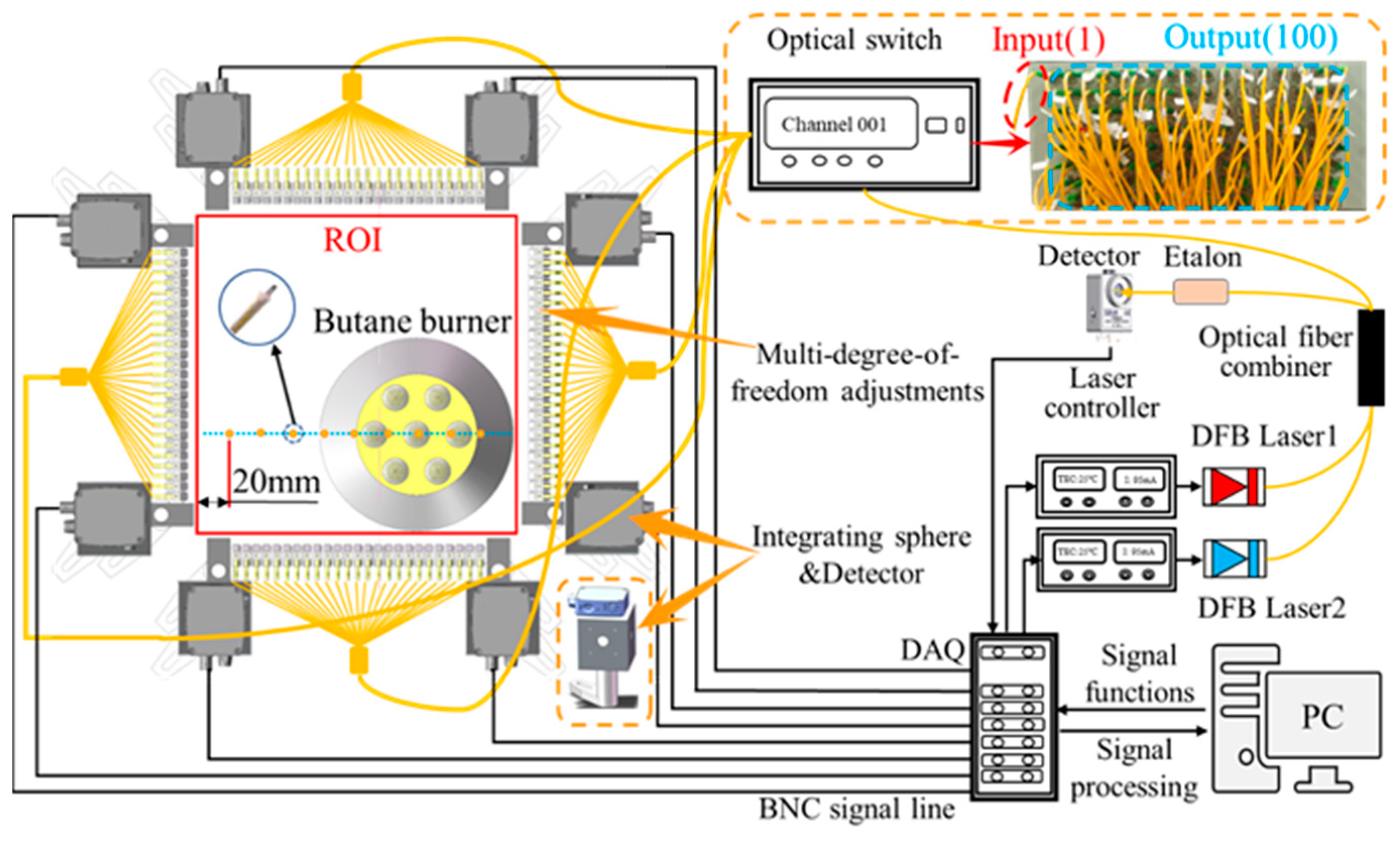
4.1. Experimental Setup

In order to validate the proposed method, an image of the temperature distribution of a combustion field was reconstructed. The temperature distribution was generated by a butane burner. As shown in Figure 16, the test system consists of a laser source, a butane burner, a K-type thermocouple (HH-K-24-SLE), a light switch (customized), a sensor and a host computer.

The laser beam was generated by two distributed feedback (DFB) diodes. Two central wave frequencies of 7185.60 cm⁻¹ (NTT, NLK1E5GAAA) and 7444.36 cm⁻¹ (NTT, NLK1B5EAAA) were used, which are in the vicinity of the central spectral absorption line of H₂O molecules. The temperature–current drive of the lasers was realized by external input voltage signals to two laser drivers (Stanford DC-501) [35,36,37]. In order to realize the laser wavelength modulation, the voltage signal input to the two laser drivers was generated by a data acquisition device (DAQ, NI, PCI-6115). This voltage signal is a 1 kHz sinusoidal sweep signal superimposed on a 100 kHz sinusoidal modulation signal. The two laser beams were split into two beams by a 2 × 2 single-mode fiber coupler. One laser beam is passed through a standard lens with a free spectral range (FSR) of 0.01 cm⁻¹ for wavelength monitoring, while the other laser beam is guided to an optical multiplexer for scanning control. For one input, the optical multiplexer has 100 output channels, and the scanning interval is 10ms/per channel. The switching loss is only 0.2 dB per channel. A detailed description of the experiment is given in the literature [38,39,40]. The experimental test area was 200 mm × 200 mm, with a total grid division number of 120 × 120, with each grid having a size of 1.67 mm × 1.67 mm.

The 3D model and partial view of the butane torch burner experimental platform are shown in Figure 17a,b, and Figure 17c,d provide photographs of the experimental combustion flame and its focused view. Nine K-type thermocouples were spaced evenly (20 mm in between) over the same cross-section location. The measurements taken from the thermocouples were used as the temperature distribution references to evaluate the reconstruction accuracy of the proposed method. The field optical path arrangement is given in Figure 17e. The laser beam was arranged according to the optimal layout of the optical path for the field measurement. The overall test system can accommodate a multi-angle arrangement for 100 laser beams.

4.2. Experimental Validation and Analysis

Figure 18 shows the reconstruction results using the four different reconstruction algorithms for the temperature field generated with the butane burner. The upper part of the figure shows the 3D distribution of the reconstruction results, and the lower part of the figure shows the corresponding isothermal contour maps. In these figures, the peak value of the reconstructed flame distribution using the ART and Landweber algorithms is obviously low, and the fluctuations at the edge are more severe, whilst with MARRT and MIARO, the reconstructed images effectively represent the true temperature distribution in the high-temperature region. However, the MIARO algorithm performs better than MARRT in the flame’s center section.

The temperature values obtained using different algorithms for the corresponding cross-section in Figure 18 are shown in Figure 19. The broken lines in Figure 19 represent the measurement results using the thermocouples. With the ART and Landweber algorithms, the constructed results become flattened in both high- and low-temperature zones over this cross-section, which does not truly reflect the flame distribution, whilst the reconstructed temperatures based on the MAART and MIARO algorithms are much closer to the thermocouple measurements. In fact, in general, the temperature reconstruction using MIARO has smaller deviations from the reference thermocouple measurements.

5. Conclusions

In this paper, a multi-iterative adaptive regularization optimization reconstruction algorithm (MIARO) for laser absorption spectroscopy tomography is proposed, which eliminates the cause of the problem related to a high reconstruction sensitivity to the initial value encountered by MAART. The reconstruction parameters are also introduced into the regularization, which ensures both the quality of the reconstruction target and the convergence of regularization. The effectiveness of the reconstruction with the MIARO algorithm was verified through simulation by setting axisymmetric and non-axisymmetric temperature and vapor distributions. The simulation results show that MIARO outperformed the other three algorithms using both numerical settings. To validate the noise resistance of the proposed algorithm, noise at four different levels was superposed on the signals, and MIARO exhibited the best quality compared to the other algorithms. In fact, with the MIARO algorithm applied in the non-axisymmetric simulation model, the temperature and concentration reconstruction errors were reduced by 0.010 and 0.038 compared with the MAART reconstruction algorithm; the standard deviation of the temperature reconstruction was reduced by 60.5%, and that of the concentration reconstruction was brought down by 51.0% for non-axisymmetric settings. The simulation results also confirm that the proposed new algorithm can achieve a clear boundary of the dynamic flow field, eliminate artifacts, and improve the measurement accuracy and robustness. Experiments using a butane-burner-generated flame were conducted. With the results obtained by thermocouples used as references, MIARO clearly demonstrated its advantages over the ART and Landweber algorithms. Even compared with the MAART algorithm, MIARO performed better for most of the measurement points. Actually, the average relative error of the MIARO reconstruction algorithm was 1.82%, and that of the MAART reconstruction algorithm was 2.44% in the experiments. The reconstruction algorithm is currently only used for relatively stable combustion flames in the laboratory, and further validation is required for extremely harsh combustion flames.

References

1. Liu, Q.; Zhou, B.; Cheng, R.; Zhang, J.; Zhao, R.; Dai, M.; Zhao, X.; Wang, Y. Online Monitoring Instantaneous 2D Temperature Distributions in a Furnace Using Acoustic Tomography Based on Frequency Division Multiplexing. Case Stud. Therm. Eng. 2023, 48, 103176. [Google Scholar] [CrossRef]
2. Zhang, J.; Qi, H.; Gao, B.; He, M.; Ren, Y.; Su, M.; Cai, X. Optimization of Transducer Array for Cross-Sectional Velocity Field Reconstruction in Acoustic Tomography. IEEE Trans. Instrum. Meas. 2022, 72, 4501012. [Google Scholar] [CrossRef]
3. Zhang, J.; Qi, H.; Ren, Y.; Su, M.; Cai, X. Acoustic Tomography of Temperature and Velocity Fields by Using the Radial Basis Function and Alternating Direction Method of Multipliers. Int. J. Heat Mass Transf. 2022, 188, 122660. [Google Scholar] [CrossRef]
4. Liu, Q.; Zhou, B.; Zhang, J.; Cheng, R. Development of Flue Gas Audio-Range Velocimeter Using Quadratic-Convex Frequency Sweeping. IEEE Sens. J. 2021, 21, 9777–9787. [Google Scholar] [CrossRef]
5. Bohlin, A.; Nordström, E.; Carlsson, H.; Bai, X.; Bengtsson, P.-E. Pure Rotational CARS Measurements of Temperature and Relative O2-Concentration in a Low Swirl Turbulent Premixed Flame. Proc. Combust. Inst. 2013, 34, 3629–3636. [Google Scholar] [CrossRef]
6. Wang, L.; Jiang, Y.; Qiu, R. Experimental Study of Combustion Inhibition by Trimethyl Phosphate in Turbulent Premixed Methane/Air Flames Using OH-PLIF. Fuel 2021, 294, 120324. [Google Scholar] [CrossRef]
7. Niu, Z.; Qi, H.; Shi, J.; Ren, Y.; He, M.; Zhou, W. Three-Dimensional Rapid Visualization of Flame Temperature Field via Compression and Noise Reduction of Light Field Imaging. Int. Commun. Heat Mass Transf. 2022, 137, 106270. [Google Scholar] [CrossRef]
8. Niu, Z.; Qi, H.; Gao, B.; Wei, L.; Ren, Y.; He, M.; Wang, F. Three-Dimensional Inhomogeneous Temperature Tomography of Confined-Space Flame Coupled with Wall Radiation Effect by Instantaneous Light Field. Int. J. Heat Mass Transf. 2023, 211, 124282. [Google Scholar] [CrossRef]
9. Wang, Y.; Zhou, B.; Liu, C. Sensitivity and Accuracy Enhanced Wavelength Modulation Spectroscopy Based on PSD Analysis. IEEE Photonics Technol. Lett. 2021, 33, 1487–1490. [Google Scholar] [CrossRef]
10. Cai, W.; Kaminski, C.F. Multiplexed Absorption Tomography with Calibration-Free Wavelength Modulation Spectroscopy. Appl. Phys. Lett. 2014, 104, 154106. [Google Scholar] [CrossRef]
11. Cai, W.; Kaminski, C.F. Tomographic Absorption Spectroscopy for the Study of Gas Dynamics and Reactive Flows. Prog. Energy Combust. Sci. 2017, 59, 1–31. [Google Scholar] [CrossRef]
12. Wang, Z.; Fu, P.; Chao, X. Laser Absorption Sensing Systems: Challenges, Modeling, and Design Optimization. Appl. Sci. 2019, 9, 2723. [Google Scholar] [CrossRef]
13. Sun, P.; Zhang, Z.; Li, Z.; Guo, Q.; Dong, F. A Study of Two Dimensional Tomography Reconstruction of Temperature and Gas Concentration in a Combustion Field Using TDLAS. Appl. Sci. 2017, 7, 990. [Google Scholar] [CrossRef]
14. Liu, C.; McCann, H.; Xu, L. Perspectives on Instrumentation Development for Chemical Species Tomography in Reactive-Flow Diagnosis. Meas. Sci. Technol. 2023, 34, 121002. [Google Scholar] [CrossRef]
15. Si, J.; Fu, G.; Liu, X.; Cheng, Y.; Zhang, R.; Xia, J.; Fu, Y.; Enemali, G.; Liu, C. A Spatially Progressive Neural Network for Locally/Globally Prioritized TDLAS Tomography. IEEE Trans. Ind. Inf. 2023, 19, 10554. [Google Scholar] [CrossRef]
16. Li, N.; Weng, C. Modified Adaptive Algebraic Tomographic Reconstruction of Gas Distribution from Incomplete Projection by a Two-Wavelength Absorption Scheme. Chin. Opt. Lett. 2011, 9, 061201–061205. [Google Scholar] [CrossRef]
17. Song, J.L.; Hong, Y.J.; Wang, G.Y.; Pan, H. Algebraic Tomographic Reconstruction of Two-Dimensional Gas Temperature Based on Tunable Diode Laser Absorption Spectroscopy. Appl. Phys. B-Lasers Opt. 2013, 112, 529–537. [Google Scholar] [CrossRef]
18. Xia, H.; Kan, R.; Xu, Z.; He, Y.; Liu, J.; Chen, B.; Yang, C.; Yao, L.; Wei, M.; Zhang, G. Two-Step Tomographic Reconstructions of Temperature and Species Concentration in a Flame Based on Laser Absorption Measurements with a Rotation Platform. Opt. Lasers Eng. 2017, 90, 10–18. [Google Scholar] [CrossRef]
19. Wang, Z.; Kamimoto, T.; Deguchi, Y.; Zhou, W.; Yan, J.; Tainaka, K.; Tanno, K.; Watanabe, H.; Kurose, R. Two Dimensional Temperature Measurement Characteristics in Pulverized Coal Combustion Field by Computed Tomography-Tunable Diode Laser Absorption Spectroscopy. Appl. Therm. Eng. 2020, 171, 115066. [Google Scholar] [CrossRef]
20. Wang, Z.; Deguchi, Y.; Kamimoto, T.; Tainaka, K.; Tanno, K. Pulverized Coal Combustion Application of Laser-Based Temperature Sensing System Using Computed Tomography – Tunable Diode Laser Absorption Spectroscopy (CT-TDLAS). Fuel 2020, 268, 117370. [Google Scholar] [CrossRef]
21. Goldenstein, C.S.; Strand, C.L.; Schultz, I.A.; Sun, K.; Jeffries, J.B.; Hanson, R.K. Fitting of Calibration-Free Scanned-Wavelength-Modulation Spectroscopy Spectra for Determination of Gas Properties and Absorption Lineshapes. Appl. Opt. 2014, 53, 356–367. [Google Scholar] [CrossRef] [PubMed]
22. Goldenstein, C.S.; Schultz, I.A.; Jeffries, J.B.; Hanson, R.K. Two-Color Absorption Spectroscopy Strategy for Measuring the Column Density and Path Average Temperature of the Absorbing Species in Nonuniform Gases. Appl. Opt. 2013, 52, 7950–7962. [Google Scholar] [CrossRef] [PubMed]
23. Zhang, R.; Si, J.; Enemali, G.; Bao, Y.; Liu, C. Spatially Driven Chemical Species Tomography with Size-Adaptive Hybrid Meshing Scheme. IEEE Sens. J. 2022, 22, 12728–12737. [Google Scholar] [CrossRef]
24. Bao, Y.; Zhang, R.; Enemali, G.; Cao, Z.; Zhou, B.; McCann, H.; Liu, C. Relative Entropy Regularized TDLAS Tomography for Robust Temperature Imaging. IEEE Trans. Instrum. Meas. 2021, 70, 1–9. [Google Scholar] [CrossRef]
25. Song, J.; Xin, M.; Rao, W.; Hong, Y.; Feng, G. Integral Absorbance Measurement for a Non-Uniform Flow Field Using Wavelength Modulation Absorption Spectroscopy. Appl. Opt. 2021, 60, 5056–5065. [Google Scholar] [CrossRef] [PubMed]
26. Liu, C.; Xu, L.; Chen, J.; Cao, Z.; Lin, Y.; Cai, W. Development of a Fan-Beam TDLAS-Based Tomographic Sensor for Rapid Imaging of Temperature and Gas Concentration. Opt. Express 2015, 23, 22494–22511. [Google Scholar] [CrossRef]
27. Xu, L.; Liu, C.; Jing, W.; Cao, Z.; Xue, X.; Lin, Y. Tunable Diode Laser Absorption Spectroscopy-Based Tomography System for on-Line Monitoring of Two-Dimensional Distributions of Temperature and H 2 O Mole Fraction. Rev. Sci. Instrum. 2016, 87, 013101. [Google Scholar] [CrossRef]
28. Song, J.; Hong, Y.; Xin, M.; Wang, G.; Liu, Z. Tomography System for Measurement of Gas Properties in Combustion Flow Field. Chin. J. Aeronaut. 2017, 30, 1697–1707. [Google Scholar] [CrossRef]
29. Li, N.; Lv, X.; Weng, C. Investigation of Self-Adaptive Algebraic Tomography for Gas Reconstruction in Larger Temperature Range by Multiple Wavelengths Absorption Spectroscopy. Chin. Opt. Lett. 2014, 12, 121103. [Google Scholar] [CrossRef]
30. Gordon, I.E.; Rothman, L.S.; Hill, C.; Kochanov, R.V.; Tan, Y.; Bernath, P.F.; Birk, M.; Boudon, V.; Campargue, A.; Chance, K.V.; et al. The HITRAN2016 Molecular Spectroscopic Database. J. Quant. Spectrosc. Radiat. Transf. 2017, 203, 3–69. [Google Scholar] [CrossRef]
31. Zhao, W.S.; Xu, L.J.; Huang, A.; Gao, X.; Luo, X.Z.; Zhang, H.Y.; Chang, H.T.; Cao, Z. A WMS Based TDLAS Tomographic System for Distribution Retrievals of Both Gas Concentration and Temperature in Dynamic Flames. IEEE Sens. J. 2020, 20, 4179–4188. [Google Scholar] [CrossRef]
32. Huang, A.; Cao, Z.; Zhao, W.; Zhang, H.; Xu, L. Frequency-Division Multiplexing and Main Peak Scanning WMS Method for TDLAS Tomography in Flame Monitoring. IEEE Trans. Instrum. Meas. 2020, 69, 9087–9096. [Google Scholar] [CrossRef]
33. Niu, Z.; Qi, H.; Zhu, Z.; Li, K.; Ren, Y.; He, M. A Novel Parametric Level Set Method Coupled with Tikhonov Regularization for Tomographic Laser Absorption Reconstruction. Appl. Therm. Eng. 2022, 201, 117819. [Google Scholar] [CrossRef]
34. Yu, T.; Tian, B.; Cai, W. Development of a Beam Optimization Method for Absorption-Based Tomography. Opt. Express 2017, 25, 5982. [Google Scholar] [CrossRef] [PubMed]
35. Zhang, R.; Xia, J.; Ahmed, I.; Gough, A.; Armstrong, I.; Upadhyay, A.; Fu, Y.; Enemali, G.; Lengden, M.; Johnstone, W.; et al. A Fast Sensor for Non-Intrusive Measurement of Concentration and Temperature in Turbine Exhaust. Sens. Actuators B Chem. 2023, 396, 134500. [Google Scholar] [CrossRef]
36. Tu, R.; Gu, J.; Zeng, Y.; Zhou, X.; Yang, K.; Jing, J.; Miao, Z.; Yang, J. Development and Validation of a Tunable Diode Laser Absorption Spectroscopy System for Hot Gas Flow and Small-Scale Flame Measurement. Sensors 2022, 22, 6707. [Google Scholar] [CrossRef] [PubMed]
37. Xia, J.; Enemali, G.; Zhang, R.; Fu, Y.; McCann, H.; Zhou, B.; Liu, C. FPGA-Accelerated Distributed Sensing System for Real-Time Industrial Laser Absorption Spectroscopy Tomography at Kilo-Hertz. IEEE Trans. Ind. Inf. 2023, 1–11. [Google Scholar] [CrossRef]
38. Zhao, R.; Zhou, B.; Zhang, J.; Cheng, R.; Liu, Q.; Dai, M.; Wang, B.; Wang, Y. Rapid Online Tomograph in Non-Uniform Complex Combustion Fields Based on Laser Absorption Spectroscopy. Exp. Therm. Fluid Sci. 2023, 147, 110930. [Google Scholar] [CrossRef]
39. Zhao, R.; Zhou, B.; Zhang, J.; Cheng, R.; Liu, Q.; Dai, M.; Wang, B.; Wang, Y. A Stability and Spatial-Resolution Enhanced Laser Absorption Spectroscopy Tomographic Sensor for Complex Combustion Flame Diagnosis. Case Stud. Therm. Eng. 2023, 41, 102662. [Google Scholar] [CrossRef]
40. Zhao, R.; Zhou, B.; Liu, Q.; Dai, M.; Wang, B.; Wang, Y. Online tomography algorithm based on laser absorption spectroscopy. Acta Phys. Sin. 2023, 72, 054206. [Google Scholar] [CrossRef]
Figure 1. Flowchart of MIARO algorithm.
Applsci 13 12083 g001
Figure 2. Absorbance and line intensity ratio of selected spectral lines: (a) 7185.60 cm−1 and (b) 7444.36 cm−1. (c) The line intensities and line intensity ratios of the two spectral lines.
Applsci 13 12083 g002
Figure 3. Simulated non-uniformly distributed regions of (a) axisymmetric temperature distribution, (b) axisymmetric H2O concentration distribution, (c) non-axisymmetric temperature distribution and (d) non-axisymmetric H2O concentration distribution.
Applsci 13 12083 g003
Figure 4. Temperature and concentration field reconstruction results and errors for axisymmetric distribution with different algorithms (a,b) ART iterative algorithm, (c,d) Landweber iterative algorithm, (e,f) MAART iterative algorithm, (g,h) MIARO iterative algorithm.
Applsci 13 12083 g004
Figure 5. Comparison of reconstruction results of axisymmetric peak center section: (a) temperature reconstruction; (b) concentration reconstruction.
Applsci 13 12083 g005
Figure 6. Temperature reconstruction results for axisymmetric distribution of different noise levels.
Applsci 13 12083 g006
Figure 7. Concentration reconstruction results for different noise levels with axisymmetric distribution.
Applsci 13 12083 g007
Figure 8. Effect of noise in axisymmetric distribution on various algorithms. (a) ARE and standard deviation of temperature reconstruction results; (b) ARE and standard deviation of concentration reconstruction results.
Applsci 13 12083 g008
Figure 9. Effect of noise in axisymmetric distribution on various algorithms. (a) ARMSE and standard deviation of temperature reconstruction results; (b) ARMSE and standard deviation of concentration reconstruction results.
Applsci 13 12083 g009
Figure 10. Temperature and concentration field reconstruction results and errors for different algorithms non-axisymmetric model: (a,b) ART iterative algorithm, (c,d) Landweber iterative algorithm, (e,f) MAART iterative algorithm, (g,h) MIARO iterative algorithm.
Applsci 13 12083 g010
Figure 11. Comparison of cross-section center reconstruction results: (a) temperature reconstruction values; (b) concentration reconstruction values.
Applsci 13 12083 g011
Figure 12. Temperature reconstruction results for non-axisymmetric distribution with different noise levels.
Applsci 13 12083 g012
Figure 13. Concentration reconstruction results for non-axisymmetric distribution with different noise levels.
Applsci 13 12083 g013
Figure 14. Effect of noise properties for non-axisymmetric distribution on various algorithms. (a) ARE and standard deviation of temperature reconstruction results; (b) ARE and standard deviation of concentration reconstruction results.
Applsci 13 12083 g014
Figure 15. Effect of noise properties of non-axisymmetric models on various algorithms. (a) ARMSE and standard deviation of temperature reconstruction results; (b) ARMSE and standard deviation of concentration reconstruction results.
Applsci 13 12083 g015
Figure 16. Butane burner experimental test system.
Applsci 13 12083 g016
Figure 17. Experimental platform of the butane torch burner. (a) Three-dimensional model of the experimental platform; (b) local view of the model; (c) experimental platform photo; (d) photo of local flame view; (e) field optical path arrangement.
Applsci 13 12083 g017
Figure 18. Reconstruction results of different reconstruction algorithms for butane torch.
Applsci 13 12083 g018
Figure 19. Temperature measurements using different reconstruction algorithms at the flame center cross-section.
Applsci 13 12083 g019