Analytical Studies on Approximate Lag and Anticipating Synchronization in Two Unidirectionally Coupled Hyperchaotic Chen Systems without Time Delay

Abstract

In this paper, approximate lag synchronization (LS) and anticipating synchronization (AS) between two unidirectionally coupled hyperchaotic Chen systems without time-delay coupling are analytically investigated. Firstly, the synchronization condition for exact LS in two unidirectionally coupled hyperchaotic Chen systems with time delay in signal transmission is analytically obtained. Under such conditions, approximate LS and AS are discussed by replacing the true time-delay terms with their Taylor expansions up to the third order.Differently from other research studies, the condition for exact LS is derived by regarding LS as a special type of generalized synchronization (GS), which has nothing to do with the value of the time delay. It is convenient to individually change the value of the lag and anticipation time of approximate LS and AS without considering the synchronization condition. Our study shows the power of a new method for recreating the past signals or predicting the future signals of a hyperchaotic Chen system by using its current signals. The results provide a simple way to eliminate the negative effects of time delay in the signal transmission between two hyperchaotic systems.

1. Introduction

The synchronization of chaotic systems plays a tremendous role in nonlinear system analysis and has been applied in a large variety of physical, chemical, neural network and biological systems [1,2,3] since the pioneering work of Pecora and Carroll [4]. The synchronization of chaotic systems is a process wherein two chaotic systems adjust a certain characteristic of their motion to standard performance because of a coupling or a forcing. Many different synchronization regimes have been studied in the past several decades, for instance, complete (or identical) synchronization (CS) [5,6], phase synchronization (PS) [7], lag synchronization (LS) [8,9,10,11,12], generalized synchronization (GS) [13,14], anticipating synchronization (AS) [15,16,17] and so on. Among all types of synchronization, CS is the simplest one, where the states of all oscillators are identical. GS is considered to be the type of chaos synchronization most frequently occurring in natural systems and is characterized by the existence of a functional relation between the state variables of drive–response systems. Different types of synchronization, such as CS, LS and AS, can be viewed as special types of GS with different functional relations.

In technology and nature, the time delay is ubiquitous due to finite signal transmission times, switching speeds as well as memory effects. LS, typically appearing as a coincidence of the shifted-in-time states of two systems, has received extensive attention in secure communications [18], laser networks [9] and digital image encryption [19]. AS was firstly proposed by Voss [20,21], who considered two chaotic systems unidirectionally coupled in a drive–response configuration and showed that the current states of a response system can be synchronized with the future states of a drive system. Two different coupling schemes were suggested by Voss: One is for the case where there exists an internal delay in a drive system that defines the anticipation time of a synchronized state. The other is for the case where a drive system does not possess internal delays, while in a salve system, there exists time-delay self-feedback. The work by Voss has led to the proven possibility of a real-time predictor of chaotic dynamics for systems without delays. Moreover, the scheme allows one to change the anticipation time without altering the dynamics of a drive system. As a possible application, AS can be used to design control methods for avoiding unwanted pulses from a drive system. AS has been reported in many applications in semiconductor lasers [22], chaotic laser diodes and cryptography [23,24].

Both LS and AS are mostly observed in systems using a time-delay factor. However, approximate LS has been found in bidirectionally and unidirectionally coupled oscillators with parameter mismatch [25]. AS has been also observed in systems without time delay. Such a type of phenomenon was first reported in the classical Voss scheme, where the true time-delay term was replaced with its first-order approximation [26]. Nevertheless, AS is not exact, that is, the advanced trajectory of a drive system only approximately coincides with the current trajectory of a response system. In addition, the anticipation time, in this case, is small. Blakely et al. [25] considered a more general case of nonidentical systems without time delay in which the mean frequency of a free response system is greater than the mean frequency of a master system. They showed that AS may occur in the Voss coupling scheme with vanishing time delay. If the above condition is satisfied in neural systems, the chaotic spikes of a presynaptic neuron may be predicted by a postsynaptic neuron. The Voss scheme provides a simple memoryless method to achieve LS and AS between coupled oscillators. In previous research studies on approximate LS and AS between two unidirectionally coupled chaotic systems without time-delay coupling, the true time-delay terms are first replaced by using their first-order approximations, which results in parameter mismatch between the drive and response systems. However, the value of the lag or anticipation time in approximate LS and AS significantly affects the synchronization condition for the two chaotic systems with such parameter mismatches. To guarantee synchronization, the value has to be limited to a very finite range. Furthermore, extending the result derived for two chaotic systems to larger arrays must also take into account possible instabilities caused by additional spatial modes. To overcome the disadvantage, the nature of the evolution of approximate LS and AS needs to be further studied in detail.

In this paper, approximate LS and AS between two unidirectionally coupled hyperchaotic Chen systems [27] without time-delay coupling are investigated. A hyperchaotic system is classified as a chaotic system with more than one positive Lyapunov exponent or unstable direction, which generates high complexity. We first analyze the synchronization condition for exact LS in two unidirectionally coupled hyperchaotic Chen systems with time delay in the signal transmission from the drive systems. Differently from most research studies, LS is regarded as a special type of GS, which can be studied by using the auxiliary system approach [28,29]. We show that the synchronization condition for exact LS analytically obtained in this paper is effective for any value of time delay in the signal transmission between two hyperchaotic Chen systems. Under such conditions, approximate LS and AS are discussed by replacing the true time-delay terms with their Taylor expansions up to the third order. Our research provides an effective method for recreating the past signals or predicting the future signals of a hyperchaotic Chen system by using its current signals.

The rest of this paper is organized as follows: In Section 2, two unidirectionally coupled hyperchaotic Chen systems with time delay in signal transmission are introduced. In Section 3, the synchronization condition for exact LS in the drive–response system is derived by regarding LS as a special type of GS, in which the auxiliary system approach and Laplace transform, combined with the successive approximation approach [30] in the Volterra integral equation theory, are used. In Section 4, numerical simulations are presented to verify the effectiveness of the synchronization condition for exact LS obtained in this paper. Approximate LS and AS are discussed in Section 5 and Section 6, respectively. The conclusions are finally drawn in Section 7.

2. System Description

The hyperchaotic Chen system [27] is described as follows:

$$\begin{array}{cc}\hfill & \dot{u}=a(v-u)+p,\hfill \\ \hfill & \dot{v}=du+cv-uw,\hfill \\ \hfill & \dot{w}=-bw+uv,\hfill \\ \hfill & \dot{p}=rp+vw,\hfill \end{array}$$

(1)

where $u,v,w$ and p are state variables and $a,b,c,d$ and r are real parameters. Assume that $(u_0,v_0,w_0,p_0)$ is one equilibrium point in system (1). For convenience, by moving the equilibrium to the origin, system (1) can be written as

$$\begin{array}{cc}\hfill & {\dot{x}}_1=-a{x}_1+a{x}_2+x_4,\hfill \\ \hfill & {\dot{x}}_2=\alpha x_1+c{x}_2-u_0{x}_3-x_1{x}_3,\hfill \\ \hfill & {\dot{x}}_3=v_0{x}_1+u_0{x}_2-b{x}_3+x_1{x}_2,\hfill \\ \hfill & {\dot{x}}_4=w_0{x}_2+v_0{x}_3+r{x}_4+x_2{x}_3,\hfill \end{array}$$

(2)

where $x_1=u-u_0$, $x_2=v-v_0$, $x_3=w-w_0$, $x_4=p-p_0$, and $\alpha =d-w_0$. System (2) is chosen as the drive system. The response system is given as:

$$\begin{array}{cc}\hfill & {\dot{y}}_1=-a{y}_1+a{y}_2+y_4+k_1(x_1(t-\tau )-y_1),\hfill \\ \hfill & {\dot{y}}_2=\alpha y_1+c{y}_2-u_0{y}_3-y_1{y}_3+k_2(x_2(t-\tau )-y_2),\hfill \\ \hfill & {\dot{y}}_3=v_0{y}_1+u_0{y}_2-b{y}_3+y_1{y}_2+k_3(x_3(t-\tau )-y_3),\hfill \\ \hfill & {\dot{y}}_4=w_0{y}_2+v_0{y}_3+r{y}_4+y_2{y}_3+k_4(x_4(t-\tau )-y_4),\hfill \end{array}$$

(3)

where $y_{1,2,3,4}$ are state variables, $k_{1,2,3,4}$ are coupling strengths and $\tau$ is the time delay in signal transmission between systems (2) and (3). LS in systems (2) and (3) is reached if

$$\left|\right|y_i-x_i(t-\tau )\left|\right|\to 0,i=1,2,3,4,fort\to \infty .$$

(4)

3. The Synchronization Condition for Exact LS between Systems (2) and (3)

Condition (4) is a functional relation between $y_i$ and $x_i$, $i=1,2,3,4$. Then, LS between systems (2) and (3) can be regarded as a special type of GS between them, which can be investigated by using the auxiliary system approach [28]. The auxiliary system corresponding to systems (2) and (3) is given by

$$\begin{array}{cc}\hfill & {\dot{z}}_1=-a{z}_1+a{z}_2+z_4+k_1(x_1(t-\tau )-z_1),\hfill \\ \hfill & {\dot{z}}_2=\alpha z_1+c{z}_2-u_0{z}_3-z_1{z}_3+k_2(x_2(t-\tau )-z_2),\hfill \\ \hfill & {\dot{z}}_3=v_0{z}_1+u_0{z}_2-b{z}_3+z_1{z}_2+k_3(x_3(t-\tau )-z_3),\hfill \\ \hfill & {\dot{z}}_4=w_0{z}_2+v_0{z}_3+r{z}_4+z_2{z}_3+k_4(x_4(t-\tau )-z_4),\hfill \end{array}$$

(5)

where $z_{1,2,3,4}$ are state variables. The following condition is necessary to obtain condition (4):

$$\left|\right|y_i-z_i\left|\right|\to 0,i=1,2,3,4,fort\to \infty .$$

(6)

By letting

$$e_i=\frac{y_i-z_i}{2},e_{i+4}=\frac{y_i+z_i}{2},i=1,2,3,4,$$

the synchronization error system for condition (6) can be given as

$$\begin{array}{cc}\hfill & {\dot{e}}_1=-(k_1+a)e_1+a{e}_2+e_4,\hfill \\ \hfill & {\dot{e}}_2=\alpha e_1+(c-k_2)e_2-u_0{e}_3-e_1{e}_7-e_3{e}_5,\hfill \\ \hfill & {\dot{e}}_3=v_0{e}_1+u_0{e}_2-(b+k_3)e_3+e_1{e}_6+e_2{e}_5,\hfill \\ \hfill & {\dot{e}}_4=w_0{e}_2+v_0{e}_3+(r-k_4)e_4+e_2{e}_7+e_3{e}_6.\hfill \end{array}$$

(7)

Condition (6) becomes

$$\left|\right|e_i\left|\right|\to 0,i=1,2,3,4,fort\to \infty .$$

(8)

Consider the Laplace transform, defined as follows:

$$\begin{array}{cc}\hfill & E_i\left(s\right)=L\left[e_i\right]={\int }_0^{+\infty }{e}_i\left(t\right)e^{-st}dt,\hfill \\ \hfill & e_i\left(t\right)=L^{-1}\left[E_i\right]=\frac{1}{2\pi j}{\int }_{\sigma -j\infty }^{\sigma +j\infty }{E}_i\left(s\right)e^{st}ds,i=1,2,3,4.\hfill \end{array}$$

(9)

By taking the Laplace transform on both sides of system (7), it yields

$$\left(s{I}_4-M\right)\left[\begin{array}{c}{E}_1\\ E_2\\ E_3\\ E_4\end{array}\right]=\left[\begin{array}{c}{e}_{10}\\ W_1+e_{20}\\ W_2+e_{30}\\ W_3+e_{40}\end{array}\right]$$

(10)

where $e_{0i}$, $i=1,2,3,4$ are the given initial values for system (7), $I_4$ is the $4\times 4$ identity real matrix,

$$M=\left[\begin{array}{cccc}-k_1-a& a& 0& 1\\ \alpha & c-k_2& -u_0& 0\\ v_0& u_0& -b-k_3& 0\\ 0& w_0& v_0& r-k_4\end{array}\right]$$

(11)

and $W_i$, $i=1,2,3$ are the Laplace transform of the nonlinear parts in the last three equations in system (7), respectively,

$$\begin{array}{cc}\hfill & W_1=-{\int }_0^{+\infty }[e_1{e}_7+e_3{e}_5]e^{-st}dt,\hfill \\ \hfill & W_2={\int }_0^{+\infty }[e_1{e}_6+e_2{e}_5]e^{-st}dt,\hfill \\ \hfill & W_3={\int }_0^{+\infty }[e_2{e}_7+e_3{e}_6]e^{-st}dt.\hfill \end{array}$$

Solving Equation (10) by using Cramer’s rule, one has

$$\begin{array}{cc}\hfill & E_1=\frac{1}{D\left(s\right)}\left|\begin{array}{cccc}{e}_{10}& a& 0& 1\\ W_1+e_{20}& c-k_2& -u_0& 0\\ W_2+e_{30}& u_0& -b-k_3& 0\\ W_3+e_{40}& w_0& v_0& r-k_4\end{array}\right|,\hfill \\ \hfill & E_2=\frac{1}{D\left(s\right)}\left|\begin{array}{cccc}-k_1-a& e_{10}& 0& 1\\ \alpha & W_1+e_{20}& -u_0& 0\\ v_0& W_2+e_{30}& -b-k_3& 0\\ 0& W_3+e_{40}& v_0& r-k_4\end{array}\right|,\hfill \\ \hfill & E_3=\frac{1}{D\left(s\right)}\left|\begin{array}{cccc}-k_1-a& a& e_{10}& 1\\ \alpha & c-k_2& W_1+e_{20}& 0\\ v_0& u_0& W_2+e_{30}& 0\\ 0& w_0& W_3+e_{40}& r-k_4\end{array}\right|,\hfill \end{array}$$

$$\begin{array}{cc}\hfill & E_4=\frac{1}{D\left(s\right)}\left|\begin{array}{cccc}-k_1-a& a& 0& e_{10}\\ \alpha & c-k_2& -u_0& W_1+e_{20}\\ v_0& u_0& -b-k_3& W_2+e_{30}\\ 0& w_0& v_0& W_3+e_{40}\end{array}\right|,\hfill \end{array}$$

(12)

where

$$D\left(s\right)=s^4+{\beta }_1{s}^3+{\beta }_2{s}^2+{\beta }_{3}s+{\beta }_4,$$

(13)

$$\begin{array}{cc}\hfill & {\beta }_1=a+b-c-k-r,\hfill \\ \hfill & {\beta }_2=\left(b-\alpha -c-r\right)a-\left(c+k+r\right)b+\left(k+r\right)c+kr+{{\mathit{u}}_{\mathit{0}}}^2,\hfill \\ \hfill & {\beta }_3=\left(a-k-r\right){{\mathit{u}}_{\mathit{0}}}^2+a{\mathit{u}}_{\mathit{0}}{\mathit{v}}_{\mathit{0}}+\left((\alpha +c)r-\left(\alpha +c+r\right)b\right)a+\left(ck+rc+kr\right)b\hfill \\ \hfill & -krc-\alpha {\mathit{w}}_{\mathit{0}}-{{\mathit{v}}_{\mathit{0}}}^2,\hfill \\ \hfill & {\beta }_4=r\left(k-a\right){{\mathit{u}}_{\mathit{0}}}^2+\left({\mathit{w}}_{\mathit{0}}-ar-\alpha \right){\mathit{u}}_{\mathit{0}}{\mathit{v}}_{\mathit{0}}+c{{\mathit{v}}_{\mathit{0}}}^2+\left(\alpha +c\right)abr-\left(krc+\alpha {\mathit{w}}_{\mathit{0}}\right)b.\hfill \end{array}$$

$D\left(s\right)$ is just the characteristic polynomial of matrix (11). In fact, we do not need to know the actual formulas of the numerators of $E_i$, $i=1,2,3,4$. They must have the following forms:

$$E_i=\frac{h_{i0}\left(s\right)}{D\left(s\right)}+\sum _{j=1}^3\frac{h_{ij}\left(s\right)}{D\left(s\right)}{W}_j,i=1,2,3,4,$$

(14)

in which $h_{ij}\left(s\right)$ ($i=1,2,3,4$, $j=0,1,2,3$) are polynomials of s whose orders are less than four. Taking the inverse Laplace transform for $E_i$, $i=1,2,3,4$ and considering the convolution theorem in the Laplace transform produces

$$\begin{array}{cc}\hfill & e_i={\gamma }_{i0}\left(t\right)-{\int }_0^t{\gamma }_{i1}(t-\tau )[e_1{e}_7+e_3{e}_5]d\tau +{\int }_0^t{\gamma }_{i2}(t-\tau )[e_1{e}_6+e_2{e}_5]d\tau \hfill \\ \hfill & +{\int }_0^t{\gamma }_{i3}(t-\tau )[e_2{e}_7+e_3{e}_6]d\tau ,i=1,2,3,4,\hfill \end{array}$$

(15)

where ${\gamma }_{ij}\left(t\right)=L^{-1}\left[\frac{h_{ij\left(s\right)}}{D\left(s\right)}\right]$, $i=1,2,3,4$ and $j=0,1,2,3$. If the denominator $D\left(s\right)$ in Equation (14) can be decomposed into $D\left(s\right)=Q_1\left(s\right)Q_2\left(s\right)$, and $Q_{1,2}$ have no common factors, then $h_{ij}\left(s\right)/D\left(s\right)$, $i\in \{1,2,3,4\}$, $j\in \{0,1,2,3\}$ can be decomposed into

$$\frac{h_{ij}\left(s\right)}{D\left(s\right)}=\frac{{\overline{h}}_{ij}\left(s\right)}{Q_1\left(s\right)}+\frac{{\widehat{h}}_{ij}\left(s\right)}{Q_2\left(s\right)},i\in \{1,2,3,4\},j\in \{0,1,2,3\},$$

where ${\overline{h}}_{ij}\left(s\right)$ and ${\widehat{h}}_{ij}\left(s\right)$ are polynomials of s. Moreover, the highest powers are less than those of $Q_1\left(s\right)$ and $Q_2\left(s\right)$. One can continue the process until only the following two classes of functions retain

$$\frac{A_1\left(s\right)}{{(s-{\eta }_0)}^m},\frac{A_2\left(s\right)}{{(s^2+{\eta }_{1}s+{\eta }_2)}^n},$$

in which $m\in \{1,2,3,4\}$, $n\in \{1,2\}$, ${\eta }_{0,1,2}\in R$, ${\eta }_1^2-4{\eta }_2<0$ and the highest powers of polynomials $A_{1,2}$ are less than m and n, respectively. Consider the inverse Laplace transform in the following three cases:

• $\frac{A_1\left(s\right)}{{(s-{\eta }_0)}^m}=\frac{B_1}{s-{\eta }_0}+\frac{B_2}{{(s-{\eta }_0)}^2}+\cdots +\frac{B_m}{{(s-{\eta }_0)}^m}$,
  where $B_{(m-i)}=\frac{1}{i!}\frac{d^i}{d{s}^i}\left[\frac{A_1\left(s\right)}{{(s-{\eta }_0)}^m}{(s-{\eta }_0)}^m\right]{|}_{s={\eta }_0}$, $i=1,2,\cdots ,m-1$,
  $B_m=\left[\frac{A_1\left(s\right)}{{(s-{\eta }_0)}^m}{(s-{\eta }_0)}^m\right]{|}_{s={\eta }_0}$,
  $L^{-1}\left[\frac{A_1\left(s\right)}{{(s-{\eta }_0)}^m}\right]=(B_1+B_{2}t+B_3{t}^2+\cdots +B_m{t}^{m-1})e^{{\eta }_{0}t}$
• $\frac{A_2\left(s\right)}{s^2+{\eta }_{1}s+{\eta }_2}=\frac{A_2\left(s\right)}{(s-{\omega }_1-j{\omega }_2)(s-{\omega }_1+j{\omega }_2)}=\frac{B_1}{s-{\omega }_1-j{\omega }_2}+\frac{B_2}{s-{\omega }_1+j{\omega }_2}$,
  where $B_{1,2}=\frac{A_2\left(s\right)}{2s+{\eta }_1}{|}_{s={\omega }_1\pm j{\omega }_2}$,
  $L^{-1}\left[\frac{A_2\left(s\right)}{s^2+{\eta }_{1}s+{\eta }_2}\right]=B_1{e}^{({\omega }_1+j{\omega }_2)t}+B_2{e}^{({\omega }_1-j{\omega }_2)t}$
• $\frac{A_2\left(s\right)}{{(s^2+{\eta }_{1}s+{\eta }_2)}^2}=\frac{B_1}{{(s-{\omega }_1-j{\omega }_2)}^2}+\frac{B_2}{s-{\omega }_1-j{\omega }_2}+\frac{B_3}{{(s-{\omega }_1+j{\omega }_2)}^2}+\frac{B_4}{s-{\omega }_1+j{\omega }_2}$,
  where $B_{1,3}=\frac{A_2\left(s\right)}{s^2+{\eta }_{1}s+{\eta }_2}{(s-{\omega }_1\pm j{\omega }_2)}^2{|}_{s={\omega }_1\pm j{\omega }_2}$,
  $B_{2,4}=\frac{d}{ds}\left[\frac{A_2\left(s\right)}{s^2+{\eta }_{1}s+{\eta }_2}{(s-{\omega }_1\pm j{\omega }_2)}^2\right]{|}_{s={\omega }_1\pm j{\omega }_2}$,
  $L^{-1}\left[\frac{A_2\left(s\right)}{{(s^2+{\eta }_{1}s+{\eta }_2)}^2}\right]=(B_{1}t+B_2)e^{({\omega }_1+j{\omega }_2)t}+(B_{3}t+B_4)e^{({\omega }_1-j{\omega }_2)t}$

From Equation (15), the necessary conditions for $\left|\right|e_i\left|\right|\to 0$, $i=1,2,3,4$ are ${\gamma }_{ij}\left(t\right)\to 0$, $i\in \{1,2,3,4\}$ and $j\in \{0,1,2,3\}$. According to the above analysis for the inverse Laplace transform, all eigenvalues of matrix (11) should have negative real parts. Under such conditions, when $t\to 0$ system (15) becomes

$$\begin{array}{cc}\hfill & e_i=-{\int }_0^t{\gamma }_{i1}(t-\tau )[e_1{e}_7+e_3{e}_5]d\tau +{\int }_0^t{\gamma }_{i2}(t-\tau )[e_1{e}_6+e_2{e}_5]d\tau \hfill \\ \hfill & +{\int }_0^t{\gamma }_{i3}(t-\tau )[e_2{e}_7+e_3{e}_6]d\tau ,i=1,2,3,4.\hfill \end{array}$$

(16)

Actually, these are a set of Volterra integral equations in system (16) that can be solved based on the successive approximation method [30]. For the sake of clarity, we briefly introduce the successive approximation method below. Consider the integral equation of the following form

$$y\left(t\right)=\Phi \left(t\right)+{\int }_0^{t}g(t-\tau )h(\tau ,y(\tau \left)\right)d\tau ,$$

(17)

where g is an $n\times n$ matrix; $\Phi \left(t\right)$ and $h(t,y(t\left)\right)$ are vectors with n components. If the following conditions are satisfied, then Equation (17) has a unique continuous solution:

• $\left|y\right|<\infty$;
• $\Phi$ and h are continuous for $0<t<t_0$, in which $0<t_0<+\infty$;
• $\left|g\right|\in L[0,ϵ]$ holds for any $0<ϵ<t_0$;
• For any $\xi >0$, if $|y_1-y_2| <\xi$ there must exist a constant $ϵ>0$ such that $|h(t,y_1)-h(t,y_2)| <ϵ$.

Moreover, the following successive approximations

$${\omega }_0\left(t\right)=0,{\omega }_{n+1}\left(t\right)=\Phi \left(t\right)+{\int }_0^{t}g(t-\tau )h(\tau ,{\omega }_n\left(\tau \right))d\tau ,n=0,1,2,\cdots$$

(18)

will uniformly converge to the unique continuous solution to Equation (17).

It is clear that the functions and parameters in Equation (16) satisfy the assumptions for Equation (17). Then, Equation (16) has the unique continuous solution $e_i=0$, $i=1,2,3,4$.

Remark 1.

The steps required to derive the synchronization condition for CS between systems (3) and (5) are listed below:

• System (7) is obtained with variable substitution;
• Through the Laplace transform and the convolution theorem, system (7) is converted into a set of Volterra integral equations (system(15)), which can be further simplified to Equation (16) based on the convergence requirement;
• The successive approximation method [30] is used to solve Equation (16). Then, the synchronization condition for CS between systems (3) and (5) is determined.

Remark 2.

The condition that all roots of $D\left(s\right)$ defined in Equation (13) have negative real parts guarantees the occurrence of CS between systems (3) and (5). $D\left(s\right)$ is the characteristic polynomial of matrix (11). From the auxiliary system approach, under such conditions the functional relationship $y_i=x_i(t-\tau )$, $i=1,2,3,4$ will be achieved between systems (2) and (3).

Remark 3.

According to the Routh–Hurwitz criteria, the necessary and sufficient condition that all roots of $D\left(s\right)$ have negative real parts can be written as

$${\beta }_1>0,{\beta }_3>0,{\beta }_4>0,and{\beta }_1{\beta }_2{\beta }_3>{\beta }_3^2+{\beta }_1^2{\beta }_4.$$

(19)

In particular, if $u_0=v_0=w_0=p_0=0$, Equation (13) becomes

$$D\left(s\right)=[s^2+(k_1+k_2-c+a)s+(k_1+a)(k_2-c)-ad](s+k_3+b)(s+k_4-r).$$

(20)

Condition (19) can be written as:

$$k_1+k_2>a-c,(k_1+a)(k_2-c)-ad>0,k_3<-b,and{k}_4>r.$$

(21)

Remark 4.

The time delay τ has nothing to do with conditions (19) or (21), which implies that the synchronization condition obtained in this paper is effective for any value of τ. In the next section, we numerically verify the effectiveness of condition (21).

4. Numerical Simulations

In this section, numerical simulations are carried out to verify the effectiveness of the criterion obtained in the previous section for the appearance of LS between systems (2) and (3). When $a=35$, $b=3$, $c=12$, $d=7$ and $0\le r\le 0.085$, system (1) is chaotic; when $a=35$, $b=3$, $c=12$, $d=7$ and $0.085<r\le 0.798$, system (1) is hyperchaotic; and when $a=35$, $b=3$, $c=12$, $d=7$ and $0.798<r\le 0.90$, system (1) is periodic. In the following, we consider the hyperchaotic case. By calculation, when $a=35$, $b=3$, $c=12$, $d=7$ and $0.085<r\le 0.798$, the hyperchaotic Chen system (1) only has one equilibrium $(0,0,0,0)$.

In the following simulations, the parameters in systems (2), (3) and (5) are taken as $a=35$, $b=3$, $c=12$, $d=7$ and $r=0.5$. From condition (21), the functional relationship $y_i=x_i(t-\tau )$, $i=1,2,3,4$ between systems (2) and (3) can be achieved if one chooses $k_1=0$, $k_2=19$, $k_3=-2$ and $k_4=0.6$. The numerical results are presented in Figure 1, Figure 2, Figure 3 and Figure 4 for different values of the time delay $\tau$, where the initial conditions are taken as $x_1(-\tau ,0]=0.1$; $x_2(-\tau ,0]=0.2$; $x_3(-\tau ,0]=0.3$; $x_4(-\tau ,0]=0.4$; $y_1(-\tau ,0]=0.2$; $y_2(-\tau ,0]=0.2$; $y_3(-\tau ,0]=0.3$; $y_4(-\tau ,0]=0.4$; $z_1(-\tau ,0]=0.3$; $z_2(-\tau ,0]=0.4$; $z_3(-\tau ,0]=0.3$; and $z_4(-\tau ,0]=0.4$. It is depicted that the synchronization errors $y_i-z_i$, $i=1,2,3,4$ between systems (3) and (5) approach zero and the functional relation $y_i=x_i(t-\tau )$, $i=1,2,3,4$ between systems (2) and (3) can be achieved for different values of the time delay: $\tau =0$, $0.2$, 1 and 2, respectively. The time delay in the signal transmission results in the transition from CS to LS between two hyperchaotic Chen systems under condition (21). In fact, the synchronization condition obtained in this paper for exact LS between systems (2) and (3) is not involved with the value of $\tau$. We show in Figure 5 that even if the value of $\tau$ is extremely large, exact LS between systems (2) and (3) still can be achieved, where the initial conditions remain as those in Figure 1, Figure 2, Figure 3 and Figure 4.

5. The Approximation of LS between Two Hyperchaotic Chen Systems without Time-Delay Coupling

The synchronization condition for exact LS between two unidirectionally coupled hyperchaotic Chen systems with time-delay coupling serves as the foundation to realize approximate LS between two unidirectionally coupled hyperchaotic Chen systems without time-delay coupling. Synchronization condition (21) is valid for any value of the time delay. Under such conditions, we replace the time-delay terms in Equation (3) with their Taylor expansions to achieve approximate LS between Equations (2) and (3).

Near $\tau =0$, $y_i=x_i(x-\tau )$, $i=1,2,3,4$, can be approximately expanded as

$$x_i(t-\tau )=x_i\left(t\right)-\frac{d{x}_i}{dt}\tau +\frac{1}{2!}\frac{d^2{x}_i}{d{t}^2}{\tau }^2-\frac{1}{3!}\frac{d^3{x}_i}{d{t}^3}{\tau }^3+O\left({\tau }^3\right),i=1,2,3,4,$$

(22)

where $O\left({\tau }^3\right)$ represents the higher order terms of $\tau$. It is theoretically possible that Equation (22) holds for any value of $\tau$. To demonstrate the feasibility of approximate LS, we define the following function of $\tau$:

$$H_i\left(\tau \right)=x_i\left(t\right)-\frac{d{x}_i}{dt}\tau +\frac{1}{2!}\frac{d^2{x}_i}{d{t}^2}{\tau }^2-\frac{1}{3!}\frac{d^3{x}_i}{d{t}^3}{\tau }^3,i=1,2,3,4.$$

(23)

$H_i\left(\tau \right)$ is the truncation up to the third order of each $x_i(t-\tau )$ in Equation (22), $i=1,2,3,4$. From system (2), one has

$$\begin{array}{cc}& \frac{d{x}_1}{dt}=-a{x}_1+a{x}_2+x_4,\hfill \\ & \frac{d^2{x}_1}{d{t}^2}=\left(-a{x}_3+a^2+ad\right)x_1+\left(-a^2+ac+x_3\right)x_2+\left(-a+r\right)x_4,\hfill \\ & \frac{d^3{x}_1}{d{t}^3}=-a{x}_2{x_1}^2+\left({x_2}^2-{x_3}^2+\left(2a^2+ab-ac+d\right)x_3-\left(a^2+ad\right)a+\left(-a^2+ac\right)d\right)x_1\hfill \\ & +\left(\left(-a^2-a-b+c+r\right)x_3+\left(a^2+ad\right)a+\left(-a^2+ac\right)c\right)x_2\hfill \\ & -a{x}_4{x}_3+\left(a^2+ad+\left(-a+r\right)r\right)x_4,\hfill \end{array}$$

(24)

$$\begin{array}{cc}& \frac{d{x}_2}{dt}=c{x}_2+d{x}_1-x_1{x}_3,\hfill \\ & \frac{d^2{x}_2}{d{t}^2}=c\left(c{x}_2+d{x}_1-x_1{x}_3\right)+(d-x_3)\left(-a{x}_1+a{x}_2+x_4\right)-x_1\left(-b{x}_3+x_1{x}_2\right),\hfill \\ & \frac{d^3{x}_2}{d{t}^3}=c\left(c\left(c{x}_2+d{x}_1-x_1{x}_3\right)+(d-x_3)\left(-a{x}_1+a{x}_2+x_4\right)-x_1\left(-b{x}_3+x_1{x}_2\right)\right)\hfill \\ & +(d-x_3)\left(-a\left(-a{x}_1+a{x}_2+x_4\right)+a\left(c{x}_2+d{x}_1-x_1{x}_3\right)+r{x}_4+x_3{x}_2\right)\hfill \\ & -2\left(-a{x}_1+a{x}_2+x_4\right)\left(-b{x}_3+x_1{x}_2\right)-x_1(-b\left(-b{x}_3+x_1{x}_2\right)\hfill \\ & +\left(-a{x}_1+a{x}_2+x_4\right)x_2+x_1\left(c{x}_2+d{x}_1-x_1{x}_3\right)),\hfill \end{array}$$

(25)

$$\begin{array}{cc}\hfill & \frac{d{x}_3}{dt}=-b{x}_3+x_1{x}_2,\hfill \\ \hfill & \frac{d^2{x}_3}{d{t}^2}=-b\left(-b{x}_3+x_1{x}_2\right)+\left(-a{x}_1+a{x}_2+x_4\right)x_2+x_1\left(c{x}_2+d{x}_1-x_1{x}_3\right),\hfill \\ \hfill & \frac{d^3{x}_3}{d{t}^3}=-b\left(-b\left(-b{x}_3+x_1{x}_2\right)+\left(-a{x}_1+a{x}_2+x_4\right)x_2+x_1\left(c{x}_2+d{x}_1-x_1{x}_3\right)\right)\hfill \\ \hfill & +\left(-a\left(-a{x}_1+a{x}_2+x_4\right)+a\left(c{x}_2+d{x}_1-x_1{x}_3\right)+r{x}_4+x_2{x}_3\right)x_2\hfill \\ \hfill & +2\left(-a{x}_1+a{x}_2+x_4\right)\left(c{x}_2+d{x}_1-x_1{x}_3\right)+x_1(c\left(c{x}_2+d{x}_1-x_1{x}_3\right)\hfill \\ \hfill & +d\left(-a{x}_1+a{x}_2+x_4\right)-\left(-a{x}_1+a{x}_2+x_4\right)x_3-x_1\left(-b{x}_3+x_1{x}_2\right)),\hfill \end{array}$$

(26)

$$\begin{array}{cc}\hfill & \frac{d{x}_4}{dt}=r{x}_4+x_2{x}_3,\hfill \\ \hfill & \frac{d^2{x}_4}{d{t}^2}=r\left(r{x}_4+x_2{x}_3\right)+\left(c{x}_2+d{x}_1-x_1{x}_3\right)x_3+x_2\left(-b{x}_3+x_1{x}_2\right),\hfill \\ \hfill & \frac{d^3{x}_4}{d{t}^3}=\left(-4x_3+3d\right)x_2{x_1}^2+(\left(r+3c-a-b\right){x_2}^2+\left(-r-c+a+3b\right){x_3}^2\hfill \\ \hfill & +\left(-ad-2db+cd+rd\right)x_3)x_1+a{x_2}^3+x_4{x_2}^2-x_4{x_3}^2+d{x}_4{x}_3+r^3{x}_4\hfill \\ \hfill & +\left(-a{x_3}^2+\left(r\left(-b+c+r\right)+ad+c^2-2cb+b^2\right)x_3\right)x_2,\hfill \end{array}$$

(27)

Replacing the time-delay terms in Equation (3) with $x_i(t-\tau )=H_i\left(\tau \right)$, $i=1,2,3,4$, yields

$$\begin{array}{cc}\hfill & {\dot{y}}_1=-a{y}_1+a{y}_2+y_4+k_1(H_1\left(\tau \right)-y_1),\hfill \\ \hfill & {\dot{y}}_2=\alpha y_1+c{y}_2-u_0{y}_3-y_1{y}_3+k_2(H_2\left(\tau \right)-y_2),\hfill \\ \hfill & {\dot{y}}_3=v_0{y}_1+u_0{y}_2-b{y}_3+y_1{y}_2+k_3(H_3\left(\tau \right)-y_3),\hfill \\ \hfill & {\dot{y}}_4=w_0{y}_2+v_0{y}_3+r{y}_4+y_2{y}_3+k_4(H_4\left(\tau \right)-y_4).\hfill \end{array}$$

(28)

Next, we investigate approximate LS between Equations (2) and (28) involving no time-delay terms. For convenience, we choose the following auxiliary system:

$$\begin{array}{cc}\hfill & {\dot{z}}_1=-a{z}_1+a{z}_2+z_4+k_1(H_1\left(\tau \right)-z_1),\hfill \\ \hfill & {\dot{z}}_2=\alpha z_1+c{z}_2-u_0{z}_3-z_1{z}_3+k_2(H_2\left(\tau \right)-z_2),\hfill \\ \hfill & {\dot{z}}_3=v_0{z}_1+u_0{z}_2-b{z}_3+z_1{z}_2+k_3(H_3\left(\tau \right)-z_3),\hfill \\ \hfill & {\dot{z}}_4=w_0{z}_2+v_0{z}_3+r{z}_4+z_2{z}_3+k_4(H_4\left(\tau \right)-z_4).\hfill \end{array}$$

(29)

By using the method presented in the previous section, GS between systems (2) and (28) with the functional relation $y_i=H_i\left(\tau \right)$, $i=1,2,3,4$ can be achieved under condition (19). As long as $H_i$ approaches $x_i(t-\tau )$, $i=1,2,3,4$, the GS between systems (2) and (28) means approximate LS between them. Numerical simulations are carried out to verify the conclusion, where the parameters remain the same as those in Figure 1, Figure 2, Figure 3, Figure 4 and Figure 5, and the initial conditions are taken as $x_1\left(0\right)=0.1$; $x_2\left(0\right)=0.2$; $x_3\left(0\right)=0.3$; $x_4\left(0\right)=0.4$; $y_1\left(0\right)=0.2$; $y_2\left(0\right)=0.2$; $y_3\left(0\right)=0.3$; $y_4\left(0\right)=0.4$; $z_1\left(0\right)=0.3$; $z_2\left(0\right)=0.4$; $z_3\left(0\right)=0.3$; and $y_4\left(0\right)=0.4$. 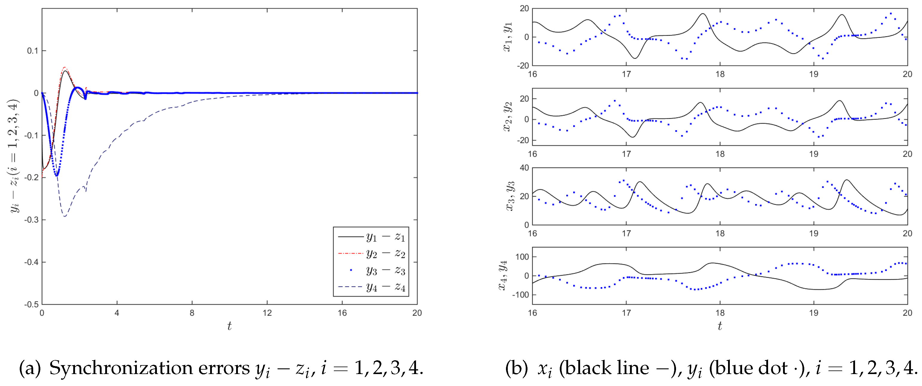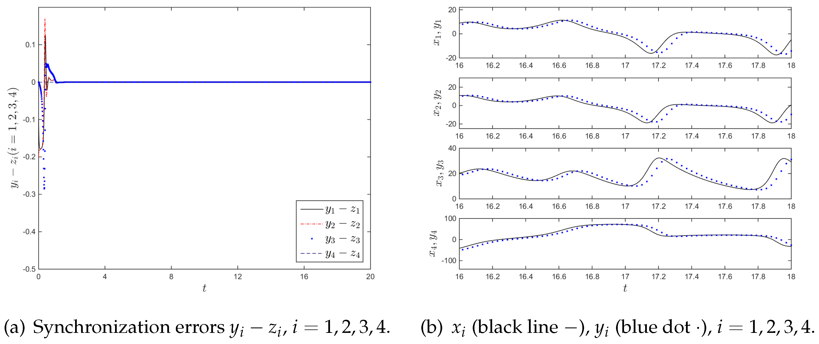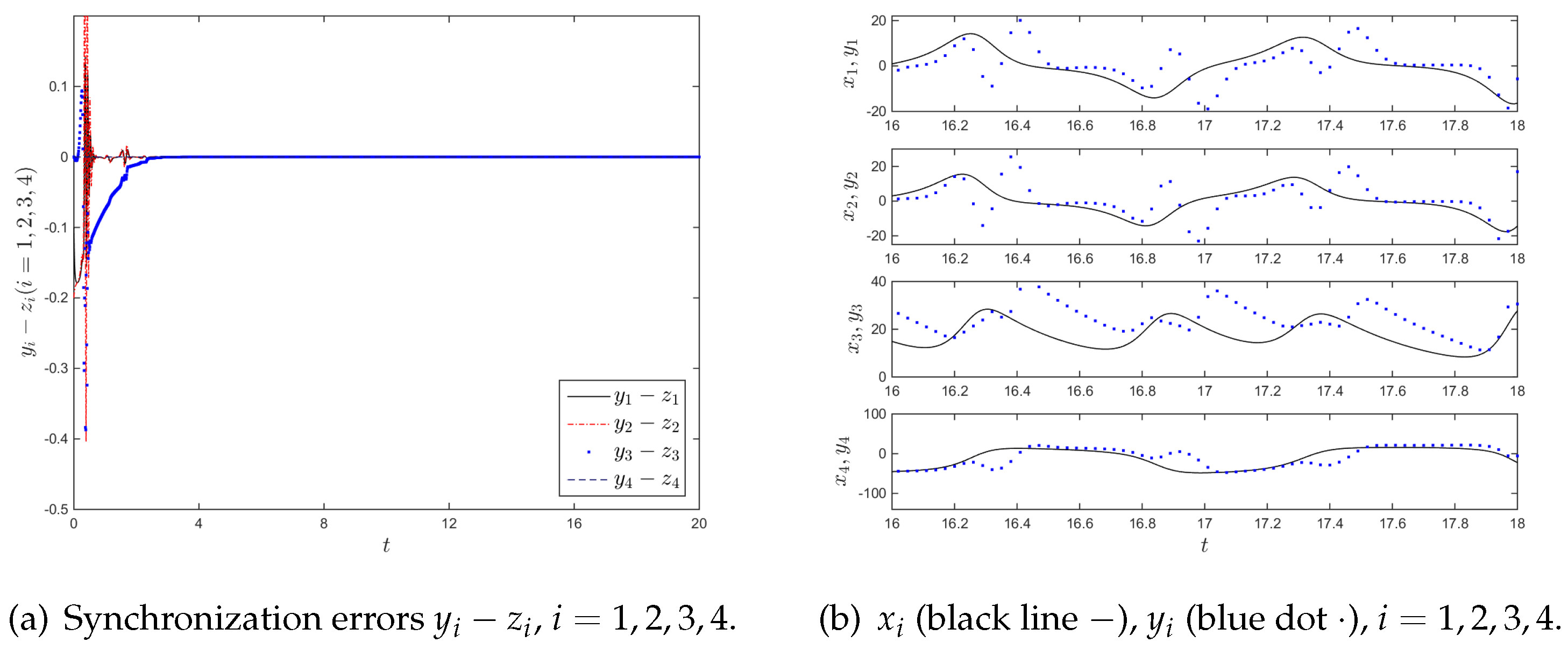The numerical results are shown in Figure 6, Figure 7, Figure 8 and Figure 9, in which the values of $\tau$ are chosen as $\tau =0.02$, $0.05$, $0.1$ and $0.15$, respectively. It is shown that for different values of $\tau$, GS always occurs between systems (2) and (28). If $\tau$ is very small (Figure 6b and Figure 7b), LS can be approximately reached between systems (2) and (28). With the increase in $\tau$, approximate LS between systems (2) and (28) is destroyed (Figure 8b and Figure 9b) because $H_i$ no longer approaches $x_i(t-\tau )$, $i=1,2,3,4$. More higher order terms of $\tau$ need to be added into Equation (23) to keep approximate LS between systems (2) and (28). Figure 6, Figure 7, Figure 8 and Figure 9 indicate that it is feasible to approximately reconstruct the past signals of a hyperchaotic Chen system by using its current signals.

6. The Approximation of AS between Two Hyperchaotic Chen Systems without Time-Delay Coupling

Consider system (2) as the drive system; systems (28) and (29) are the response and auxiliary systems, respectively. Now, we consider $\tau <0$ in the function $H_i\left(\tau \right)$, $i=1,2,3,4$ as performing the numerical simulations, where all other parameters and the initial conditions remain the same as those in the case of $\tau >0$. The numerical results are depicted in Figure 10, Figure 11, Figure 12 and Figure 13, in which the values of $\tau$ are chosen as $\tau =-0.02$, $-0.05$, $-0.1$ and $-0.15$, respectively. It is clear that GS still appears between systems (2) and (28) for different values of $\tau$ under condition (21). If $\tau$ approaches 0 (Figure 10b and Figure 11b), AS can be approximately achieved between systems (2) and (28). With the decrease in $\tau$, the approximation begins to disappear (Figure 12b and Figure 13b). To maintain approximate AS between systems (2) and (28), more higher order terms of $\tau$ need to be added into $H_i\left(\tau \right)$, $i=1,2,3,4$ in Equation (23). Figure 10, Figure 11, Figure 12 and Figure 13 imply that it is feasible to approximately predict the future signals of a hyperchaotic Chen system by using its current signals.

7. Conclusions

In this paper, approximate LS and AS in two unidirectionally coupled hyperchaotic Chen systems without time-delay coupling are analytically investigated. Firstly, the synchronization condition for exact LS between two unidirectionally coupled hyperchaotic Chen systems with time delay in signal transmission is obtained. Differently from other studies, LS is viewed as a special type of GS, which can be analyzed by using the auxiliary system approach. Based on the Laplace transform and the successive approximation method, the synchronization condition for exact LS is analytically obtained, and its effectiveness is verified using numerical simulations. Our analysis shows that the condition for exact LS is valid for any value of the time delay in signal transmission. Under such conditions, approximate LS and AS in two unidirectionally coupled hyperchaotic Chen systems without time-delay coupling are discussed by replacing the true time-delay terms with their Taylor expansions up to the third order. For a small time delay, the approximate LS and AS are precise enough. Our research indicates the possibility of recreating the past signals or predicting the future signals of a hyperchaotic Chen system using its current signals.

In previous research studies, the true time-delay terms are first replaced by using their first-order approximations. Then, synchronization conditions for approximate LS and AS are discussed by considering two chaotic systems with parameter mismatch. The lag and anticipation time of approximate LS and AS have to be involved in the synchronization condition, which are difficult to change within a wide range. In our study, the synchronization condition for exact LS between the drive and response systems with time-delay coupling is firstly obtained, which has nothing to do with the time delay. That is, the condition for exact LS is valid for any value of the time delay. Then, the value of the lag and anticipation time in approximate LS and AS can be individually varied. It is theoretically possible that any value of the lag and anticipation time in approximate LS and AS can be reached as long as there are enough truncated terms in Equation (23). The calculation of terms, of course, is tedious with the increase in truncated terms. In addition, it will become difficult to physically realize such a controller in the real world [31,32]. This is the disadvantage of the proposed scheme achieving approximate LS and AS between two undirectionally coupled hyperchaotic Chen systems without time-delay coupling.

Our research provides a simple and effective way to achieve approximate LS and AS between two hyperchaotic systems without time-delay coupling, which can be applied to eliminate the negative effects of the time delay in signal transmission.

References

1. Uchida, A.; Rogister, F.; García-Ojalvo, J.; Roy, R. Synchronization and communication with chaotic laser systems. Prog. Opt. 2005, 48, 203–341. [Google Scholar] [CrossRef]
2. Li, Y.N.; Chen, L.; Cai, Z.S.; Zhao, X. Experimental study of chaos synchronization in the Belousov–Zhabotinsky chemical system. Chaos Solitons Fractals 2004, 22, 767–771. [Google Scholar] [CrossRef]
3. Uhlhaas, P.J.; Singer, W. Neural synchrony in brain disorders: Relevance for cognitive dysfunctions and pathophysiology. Neuron 2006, 52, 155–168. [Google Scholar] [CrossRef] [PubMed]
4. Carroll, T.L.; Perora, L.M. Synchronization in chaotic systems. Phys. Rev. Lett. 1990, 64, 821–824. [Google Scholar] [CrossRef]
5. Wang, P.; Wen, G.; Yu, X.; Yu, W.; Huang, T. Synchronization of multi-layer networks: From node-to-node synchronization to complete synchronization. IEEE Trans Circuits Syst. 2018, 66, 1141–1152. [Google Scholar] [CrossRef]
6. Fatemeh, P.; Mohadeseh, S.K.; Yaser, M.; Karthikeyan, R.; Sajad, J. Complete and partial synchronization in empirical brain networks. Int. J. Electron. Commun. (AEU) 2023, 170, 154863. [Google Scholar] [CrossRef]
7. Hoon, Y.; Mohd, R.M.; Mohd, Z.M.; Zawawi, M. Shunt active power filter: A review on phase synchronization control techniques. Electronics 2019, 8, 791. [Google Scholar] [CrossRef]
8. Sun, W.; Wang, S.; Wang, G.; Wu, Y. Lag synchronization via pinning control between two coupled networks. Nonlinear Dyn. 2015, 79, 2659–2666. [Google Scholar] [CrossRef]
9. Mihana, T.; Fujii, K.; Kanno, K.; Naruse, M.; Uchida, A. Laser network decision making by lag synchronization of chaos in a ring configuration. Opt. Express 2020, 28, 40112–40130. [Google Scholar] [CrossRef]
10. Long, C.; Zhang, G.; Zeng, Z.; Hu, J. Finite-time lag synchronization of inertial neural networks with mixed infinite time-varying delays and state-dependent switching. Neurocomputing 2021, 433, 50–58. [Google Scholar] [CrossRef]
11. Ibrahim, M.M.; Kamran, M.A.; Mannan, M.M.N.; Jung, I.H.; Kim, S. Lag synchronization of coupled time-delayed Fitzhugh–Nagumo neural networks via feedback control. Sci. Rep. 2021, 11, 1–15. [Google Scholar] [CrossRef] [PubMed]
12. Rasa, S.; Loreta, S.; Minvydas, R. Detection of lag synchronization based on matrices of delayed differences. Commun. Nonlinear Sci. Numer. Simul. 2023, 116, 106864. [Google Scholar] [CrossRef]
13. Ahmadlou, M.; Adeli, H. Visibility graph similarity: A new measure of generalized synchronization in coupled dynamic systems. Physica D 2012, 241, 326–332. [Google Scholar] [CrossRef]
14. Wu, Z.; Zhang, X.; Zhong, X. Generalized chaos synchronization circuit simulation and asymmetric image encryption. IEEE Access 2019, 7, 37989–38008. [Google Scholar] [CrossRef]
15. Ciszak, M.; Mayol, C.; Mirasso, C.R.; Toral, R. Anticipated synchronization in coupled complex Ginzburg-Landau systems. Phys. Rev. E 2015, 92, 032911. [Google Scholar] [CrossRef] [PubMed]
16. Emad, E.; Mahmoud, M.; Higazy, T.M.; Al, H. A New Nine-Dimensional Chaotic Lorenz System with Quaternion Variables: Complicated Dynamics, Electronic Circuit Design, Anti-Anticipating Synchronization, and Chaotic Masking Communication Application. Mathematics 2019, 7, 877. [Google Scholar] [CrossRef]
17. Srinivasan, K.; Sivaganesh, G.; Fonzin, F.T.; Raja, M.I. Analytical studies on complete, lag and anticipation synchronization in cascaded circuits with numerical and experimental confirmation. Int. J. Electron. Commun. (AEU) 2023, 159, 154491. [Google Scholar] [CrossRef]
18. Thang, M.H.; Sanjay, K.P.; Sayan, M.; Santo, B. Synchronization and secure communication in time delayed semiconductor laser systems. Optik 2016, 127, 10930–10947. [Google Scholar] [CrossRef]
19. Kamal, F.; Elsonbaty, A.; Elsaid, A. A novel fractional nonautonomous chaotic circuit model and its application to image encryption. Chaos Solitons Fractals 2021, 144, 110686. [Google Scholar] [CrossRef]
20. Voss, H.U. Anticipating chaotic synchronization. Phys. Rev. 2000, 61, 5115. [Google Scholar] [CrossRef]
21. Voss, H.U. Dynamic long-term anticipation of chaotic states. Phys. Rev. Lett. 2001, 87, 014102. [Google Scholar] [CrossRef] [PubMed]
22. Masoller, A.P.C. Anticipation in the synchronization of chaotic semiconductor lasers with optical feedback. Phys. Rev. Lett. 2001, 86, 2782. [Google Scholar] [CrossRef] [PubMed]
23. Pyragiene, T.; Pyragas, K. Anticipating synchronization in a chain of chaotic oscillators with switching parameters. Phys. Lett. 2015, 379, 3084–3088. [Google Scholar] [CrossRef]
24. Mousa, S.K.; Al Naimee, K.A. Experimental investigations of Synchronization in two optically coupled chaotic systems utilizing optical feedback and optical injection. J. Univ. Anbar Pure Sci. 2017, 11, 49–56. [Google Scholar] [CrossRef]
25. Blakely, J.N.; Stahl, M.T.; Corron, N.J. Time-shifted synchronization of chaotic oscillator chains without explicit coupling delays. Chaos 2009, 19, 043117. [Google Scholar] [CrossRef] [PubMed]
26. Corron, N.J.; Blakely, J.N.; Pethel, S.D. Lag and anticipating synchronization without time-delay coupling. Chaos 2005, 15, 023110. [Google Scholar] [CrossRef]
27. Smaoui, N.; Karouma, A.; Zribi, M. Secure communications based on the synchronization of the hyperchaotic Chen and the unified chaotic systems. Commun. Nonlinear Sci. Numer. Simul. 2011, 16, 3279–3293. [Google Scholar] [CrossRef]
28. Abarbanel, H.D.I.; Rulkov, N.F.; Suschik, M.M. Generalized synchronization of chaos: The auxiliary system approach. Phys. Rev. E 1996, 53, 4528–4535. [Google Scholar] [CrossRef]
29. Bin, Z.; Ran, L. The study of generalized synchronization between two identical neurons based on the Laplace transform method. Appl. Sci. 2021, 11, 11774. [Google Scholar] [CrossRef]
30. Nohel, J.A. Some problems in nonlinear Volterra integral equations. Bull. Am. Math. Soc. 1962, 68, 323–330. [Google Scholar] [CrossRef]
31. Roman, R.C.; Precup, R.E.; Petriu, E.M. Hybrid data-driven fuzzy active disturbance rejection control for tower crane systems. Eur. J. Control 2021, 58, 373–387. [Google Scholar] [CrossRef]
32. Chi, R.H.; Li, H.Y.; Shen, D.; Hou, Z.S.; Huang, B. Enhanced P-type control: Indirect adaptive learning rrom set-point updates. IEEE Trans. Autom. Control 2023, 68, 1600–1613. [Google Scholar] [CrossRef]
Figure 1. (a) Synchronization errors between systems (3) and (5); (b) the time series of x i , y i , i = 1 ,   2 ,   3 ,   4 in systems (2) and (3) with k 1 = 0 , k 2 = 19 , k 3 = 2 , k 4 = 0.6 and τ = 0 .
Applsci 13 11949 g001
Figure 2. (a) Synchronization errors between systems (3) and (5); (b) the time series of x i , y i , i = 1 ,   2 ,   3 ,   4 , in systems (2) and (3) with k 1 = 0 , k 2 = 19 , k 3 = 2 , k 4 = 0.6 and τ = 0.2 .
Applsci 13 11949 g002
Figure 3. (a) Synchronizationerrors between systems (3) and (5); (b) The time series of x i , y i , i = 1 ,   2 ,   3 ,   4 , in systems (2) and (3) with k 1 = 0 , k 2 = 19 , k 3 = 2 , k 4 = 0.6 , τ = 1 .
Applsci 13 11949 g003
Figure 4. (a) Synchronization errors between systems (3) and (5); (b) the time series of x i , y i , i = 1 ,   2 ,   3 ,   4 , in systems (2) and (3) with k 1 = 0 , k 2 = 19 , k 3 = 2 , k 4 = 0.6 and τ = 2 .
Applsci 13 11949 g004
Figure 5. (a) Synchronization errors between systems (3) and (5); (b) the time series of x i , y i , i = 1 ,   2 ,   3 ,   4 , in systems (2) and (3) with k 1 = 0 , k 2 = 19 , k 3 = 2 , k 4 = 0.6 and τ = 10 .
Applsci 13 11949 g005
Figure 6. (a) Synchronization errors between systems (28) and (29). (b) The time series of x i and y i , i = 1 ,   2 ,   3 ,   4 in systems (2) and (28) with y i = H i ( τ ) ; i = 1 ,   2 ,   3 ,   4 ; k 1 = 0 ; k 2 = 19 ; k 3 = 2 ; k 4 = 0.6 ; and τ = 0.02 .
Applsci 13 11949 g006
Figure 7. (a) Synchronization errors between systems (28) and (29). (b) The time series of x i and y i , i = 1 ,   2 ,   3 ,   4 in systems (2) and (28) with y i = H i ( τ ) ; i = 1 ,   2 ,   3 ,   4 ; k 1 = 0 ; k 2 = 19 ; k 3 = 2 ; k 4 = 0.6 ; and τ = 0.05 .
Applsci 13 11949 g007
Figure 8. (a) Synchronization errors between systems (28) and (29). (b) The time series of x i and y i , i = 1 ,   2 ,   3 ,   4 in systems (2) and (28) with y i = H i ( τ ) ; i = 1 ,   2 ,   3 ,   4 ; k 1 = 0 ; k 2 = 19 ; k 3 = 2 ; k 4 = 0.6 ; and τ = 0.1 .
Applsci 13 11949 g008
Figure 9. (a) Synchronization errors between systems (28) and (29). (b) The time series of x i and y i , i = 1 ,   2 ,   3 ,   4 in systems (2) and (28) with y i = H i ( τ ) ; i = 1 ,   2 ,   3 ,   4 ; k 1 = 0 ; k 2 = 19 ; k 3 = 2 ; k 4 = 0.6 ; and τ = 0.15 .
Applsci 13 11949 g009
Figure 10. (a) Synchronization errors between systems (28) and (29). (b) The time series of x i and y i , i = 1 ,   2 ,   3 ,   4 in systems (2) and (28) with y i = H i ( τ ) ; i = 1 ,   2 ,   3 ,   4 ; k 1 = 0 ; k 2 = 19 ; k 3 = 2 ; k 4 = 0.6 ; and τ = 0.02 .
Applsci 13 11949 g010
Figure 11. (a) Synchronization errors between systems (28) and (29). (b) The time series of x i and y i , i = 1 ,   2 ,   3 ,   4 in systems (2) and (28) with y i = H i ( τ ) ; i = 1 ,   2 ,   3 ,   4 ; k 1 = 0 ; k 2 = 19 ; k 3 = 2 ; k 4 = 0.6 ; and τ = 0.05 .
Applsci 13 11949 g011
Figure 12. (a) Synchronization errors between systems (28) and (29). (b) The time series of x i and y i , i = 1 ,   2 ,   3 ,   4 in systems (2) and (28) with y i = H i ( τ ) ; i = 1 ,   2 ,   3 ,   4 ; k 1 = 0 ; k 2 = 19 ; k 3 = 2 ; k 4 = 0.6 ; and τ = 0.1 .
Applsci 13 11949 g012
Figure 13. (a) Synchronization errors between systems (28) and (29). (b) The time series of x i and y i , i = 1 ,   2 ,   3 ,   4 in systems (2) and (28) with y i = H i ( τ ) ; i = 1 ,   2 ,   3 ,   4 ; k 1 = 0 ; k 2 = 19 ; k 3 = 2 ; k 4 = 0.6 ; and τ = 0.15 .
Applsci 13 11949 g013
Disclaimer/Publisher’s Note: The statements, opinions and data contained in all publications are solely those of the individual author(s) and contributor(s) and not of MDPI and/or the editor(s). MDPI and/or the editor(s) disclaim responsibility for any injury to people or property resulting from any ideas, methods, instructions or products referred to in the content.