Datacentric Similarity Matching of Emergent Stigmergic Clustering to Fractional Factorial Vectoring: A Case for Leaner-and-Greener Wastewater Recycling

Abstract

Water scarcity is a challenging global risk. Urban wastewater treatment technologies, which utilize processes based on single-stage ultrafiltration (UF) or nanofiltration (NF), have the potential to offer lean-and-green cost-effective solutions. Robustifying the effectiveness of water treatment is a complex multidimensional characteristic problem. In this study, a non-linear Taguchi-type orthogonal-array (OA) sampler is enriched with an emergent stigmergic clustering procedure to conduct the screening/optimization of multiple UF/NF aquametric performance metrics. The stochastic solver employs the Databionic swarm intelligence routine to classify the resulting multi-response dataset. Next, a cluster separation measure, the Davies–Bouldin index, is used to evaluate input and output relationships. The self-organized bionic-classifier data-partition appropriateness is matched for signatures between the emergent stigmergic clustering memberships and the OA factorial vector sequences. To illustrate the proposed methodology, recently-published multi-response multifactorial L₉(3⁴) OA-planned experiments from two interesting UF-/NF-membrane processes are examined. In the study, seven UF-membrane process characteristics and six NF-membrane process characteristics are tested (1) in relationship to four controlling factors and (2) to synchronously evaluate individual factorial curvatures. The results are compared with other ordinary clustering methods and their performances are discussed. The unsupervised robust bionic prediction reveals that the permeate flux influences both the UF-/NF-membrane process performances. For the UF process and a three-cluster model, the Davies–Bouldin index was minimized at values of 1.89 and 1.27 for the centroid and medoid centrotypes, respectively. For the NF process and a two-cluster model, the Davies–Bouldin index was minimized for both centrotypes at values close to 0.4, which was fairly close to the self-validation value. The advantage of this proposed data-centric engineering scheme relies on its emergent and self-organized clustering capability, which retraces its appropriateness to the fractional factorial rigid structure and, hence, it may become useful for screening and optimizing small-data wastewater operating conditions.

1. Introduction

The planetary priorities for clean water and sanitation have been established by the United Nations in the Sustainable Development Goal (SDG) #6: “80% of wastewater goes into waterways without adequate treatment” [1]. “Since water stress affects more than 2 billion people (with this figure projected to increase)”, consequently, “80% of the countries have laid the foundations for integrated water resources management”. Already, more than four billion people experience the effects of water scarcity as a two-end problem: (1) water shortage due to water unavailability, and (2) water stress due to growing consumption [2,3,4]. A water footing framework facilitates the tracking down and mapping of water flows, thus permitting a resource assessment from an environmental management perspective [5,6,7]. There is a strong interplay among the different framework aspects, which implicate the dimensions of the water quantity and quality on the ‘three-colored’ water-footing avenues: (1) green (rainwater), (2) blue (ground and surface water) and (3) grey (polluted water) [8,9,10,11,12,13,14,15,16]. As agriculture may consume up to 92% of the green, blue and grey water-footing flows, this area becomes the spotlight for finding opportunities to manage water availability and consumption [17,18,19,20,21]. Grey water attracts a fair share of the evolving technological ingenuity due to the innate complexities of coping with wastewater physicochemical phenomena. Wastewater reuse is indispensable, particularly when there are great supply shortages in arid and semi-arid regions [22,23,24,25,26,27]. Improve wastewater recycling efficiency is imperative to continuously developing and optimizing a broad range of older and current separation treatments [28,29,30,31,32]. Water separation techniques that exploit the modern advances of nanofiltration and ultrafiltration processes are becoming popular in containing pollution by regulating contaminant removal from wastewater systems [33,34,35,36,37,38,39,40,41,42,43,44,45].

To achieve sustainable development goals, in an endeavor to curb pollution, innovative solutions (SDG #9) should encompass lean, green and artificial intelligence technologies, which are proven in boosting operational performance in production [46,47,48,49,50,51,52]. Green, lean and six sigma (modern quality management) practices can be the catalysts for orchestrating the manufacturing of prosperous products by optimizing upstream processes. By combining a rapid-response mentality with outcome effectuation through proper project selection rules, they are bound to assist operations in remaining profitable in a circular economy [53,54]. Generally speaking, waste reduction projects require an integrated lean–green approach to be effective in deploying and monitoring the right environmental measures and, hence, in accomplishing the aim of process performance enhancement [55,56]. Lean six sigma projects, which are supported by artificial intelligence know-how, lead to superior business results because they accelerate the innovation cycle time [57,58].

The sustainability factor is vital in improving water purification processes [59]; it stands as a broad indicator which tracks down checks and balances in production while ascertaining which operations are conducted in an environmentally sound manner. Ultrafiltration- and nanofiltration-membrane processes cover a wide range of water purity demands to complement reverse osmosis treatment capabilities. The tailored design of nanofiltration membranes can push the limits of separation by optimizing their property performance relationships [60]. At any rate, it is noted that optimizing water quality is a challenging task because of the ever-present influence and extent of uncertainty in the influx water volume [61]. A new tactic to optimize water recycling efficiency, which is chiefly intended for irrigation purposes, is to allow ultrafiltration and nanofiltration processes to compete with each other against a particular outcome [62]. Then, the most appropriate process is selected, thus achieving an optimal filtering performance. For this purpose, introducing artificial intelligence methods in screening and optimization wastewater recovery studies could unravel the arduous part of data manipulation and model prediction that wastewater treatment professionals and engineers are often confronted with [63].

An aquametric analysis is a multivariate environmental problem and, thus, it requires the implementation of formal experimental design and statistical inference methods to comprehend it [64,65]. Since the screening and optimization of recycling efficiencies are scaled at a plant level, industrial-type experimentation becomes pivotal in understanding, in an empirical way, how the specific wastewater treatment behaves. Engineers and scientists adopt fractional factorial designs (FFDs) to reduce the amount of research work by focusing on the minimization of the number of performed trials [66,67]. Clearly, it is a lean-and-green approach because it reduces: (1) the use of trial materials, (2) the waste generated from untuned processes, (3) the waste generated from unstructured product trials, (4) the industrial research manhours, (5) equipment unavailability, (6) production rescheduling and (7) the total operations research costs. FFDs also bring the agile aspect into the experimentation because they are ‘by-design’ generic, adaptable and responsive schemes and, hence, they may be applied and explained to any operational situation which is worthwhile to monitor and improve. Orthogonal arrays (OAs) are members of the FFD family of trial planners in the field of design of experiments (DOE) [66,67]. OAs have found a niche in the contemporary robust engineering philosophy, which asserts that the ‘designed-in’ quality aspect in products is redeemed with rapid product launches in the market and lower production costs [68]. A practical DOE approach, known as the Taguchi method, recommends: (1) OAs as trial planners, (2) data reduction methods based on replicate data means and signal-to-noise ratios (SNRs) and (3) analysis of variance (ANOVA) to carry out the multifactorial statistical treatment [67]. Even though the Taguchi quality philosophy suggests that the experiments should be carried out on the production line to be relevant and effective, the research activities are materialized by fast “off-line” trials. This means that the targeted process(es) should be isolated for ‘quick-gains’ research projects. Consequently, production is interrupted to divert production machinery to be utilized in experiments. Programming machinery downtime and equipment unavailability for production trials disrupts the regular production line schedule. Therefore, the industrial trials are brief, and they are executed with great urgency and the minimum possible duration.

This work will undertake the evaluation two separation systems, which rely on published ultrafiltration- and nanofiltration-membrane technologies, using a state-of-the-art artificial intelligence method. The operational demands are anticipated to impose limited access to the wastewater treatment facility for lengthy experiments to be conducted, since they would incur noticeable downtime losses. Non-linear OAs have been recommended to formulate the experimental recipes for the examined controlling factors in a published study [62]. This is because filtration phenomena may introduce curvature dependencies into the multivariate input–output relationships; non-linear OAs offer a minimum-effort opportunity to capture strong deviations from linearity. Moreover, lone replicates are planned for both the tested filtration processes in order to succeed in gaining additional resource and time savings [62]. Running the trials in the saturation mode, the experimenter aspires to extract the maximum information from the implemented OA scheme [66]. In accordance with the classical Taguchi method, the screening and optimization tasks will be conducted in a combined single effort [67]. This means extra resource and time savings are realized because a two-task project is reduced to just a single one; all data collection is completed in a single session. Meanwhile, preparing unreplicated factorial experiments in order to learn how to profile intricate water processes and improve crop yield is neither a new nor a rare prospect [69,70,71]. Nevertheless, the analysis toolset for treating generic unreplicated OA datasets is fairly elaborate and extensive [72]. It is markedly differentiated from being a simple multifactorial ANOVA exercise by the fact that saturated OAs do not permit the estimation of the experimental error.

In the illustrated case study, it is the optimal aquametric profile of a combination of irrigation water indices that is sought. Multiple water quality characteristics will be considered for both separation methods, each being relative to the specific wastewater filtration process. Statistical techniques that could handle the simultaneous screening and optimization of several process characteristics are well known and have been applied in chemical systems in the past [73,74]. This work will involve synchronous multi-characteristic aquametrics with the proviso that the investigated group of water process characteristics may be reducible to a smaller list of characteristics before the screening/optimization task commences. The ensuing reduction in output variates will be determined by the potential presence of correlations among the process characteristics and the extent of the variability within the response dataset. Moreover, the perspective will be different in this work, because the aquametric profiling will be framed such that a reverse-matching classification solution will be pursued first. No formal analysis of variance or regression methods are necessitated after this step. Technically, it is insinuated that classification may be substituted for both screening and optimization tasks in structured DOE datasets. The selection of a self-organized stochastic engine with several attractive properties is crucial to maneuver around the obscured effect of the uncertainty that is hidden behind the unreplicated, saturated, multivariate OA dataset [75,76]. The probabilities of ‘becoming’ are hinged upon the arrow of time and they are seasoned to actualities as the dual agents of emergence and self-organization take over the wheel of the proposed bionic solver. Both cultures of data analysis (statistical/algorithmic) are used to create a statistical hierarchy of the profiled effects [77]. The main component of the stochastic solver emphasizes the robustness of the implemented algorithmic engine. The most striking feature is the negation of the necessity for a global objective function to guide the solver procedure. This lessens the possibility of subjectively selecting a route to narrow down the screening/optimization path; it makes the solution more abstract and it definitely differentiates it from other smart aquametric approaches [78,79,80].

The recommended algorithm that will be tested on the non-linear OAs was devised by Thrun and Ultsch [81]. It is a swarm intelligence solver that relies on self-organization to propel the quest for an optimal clustering outcome. The solution grows out of the emergence opportunities which are bided on by the stochastic fluctuations in the scrambling databots (output data points) [82]. Even though the three-part published algorithm was developed to handle a multidimensional-scaling big-data classification problem, it is the small-and-dense data problem that is alternatively explored in this work. Regular swarm technology was not contemplated in this endeavor due to the reported issues emanating from such routines with regards to the solution accuracy in multi-objective applications and the determination of stopping criteria [81]. Clearly, by design, the preset (OA) factorial vectors are predisposed to ensure that all dataset partitions are viable in conformation to the richness property. However, the topographical map facility of the algorithm, which corrects for the two-dimensional projection of the databot assemblage errors by resorting to a hypsometric tint depiction, becomes meaningless for such a small dataset and it will not be taken advantage of.

The implemented intelligent engine will undergo a basic ‘psychometric’ pre-screening to ameliorate the ‘acumen’ of the solver. The algorithmic pre-search preparation phase will be enriched with a round of multi-response proximity analysis given that the distance function to be introduced into the routine is unknown and open to suggestions [83]. Then, the final selection of the preferred distance measure will be confirmed by optimizing the goodness-of-fit of the nominated distance measures under the nonmetric assumption [84]. Since the natural clusters are identified by similarities based on a favorable distance metric, true clusters may be retrieved. Then, the influence of each controlling factor may be backtracked by matching the clustered dataset to each individual factorial vector in an attempt to pair them through an appropriate cluster separation measure. The Davies–Bouldin index [85] will be used in a rather unorthodox manner to directly approximate the magnitude of the similarity between the clustered mini-dataset to the (OA) factorial vector element sequence that creates it. It is the OA-induced factorial ‘pre-clustering’ that offers a new way to fingerprint a clustered dataset structure. As a screening/optimization exercise, it is intriguing, because the implemented bionic technology, which is borrowed to facilitate the expediting of the multi-characteristic multifactorial analysis, it actually demonstrates that a factorial group hierarchy may emerge without piloting the solver by a debatable objective function [81], but, by using a smart combination of swarm intelligence, self-organization and non-cooperative game theory [86]. It is the intrinsic properties of randomness, irreducibility and the Nash equilibrium in non-cooperative game theory in the emergent stigmergic classification solver that solidify the non-parametric (robust) annealing scheme. The rest of the paper is organized as follows: (1) the methodology for matching the bionic optimal clustering to the OA factorial vectors is outlined, (2) the datacentric engineering analysis is presented in the Results section that covers the performance of ultra- and nano-filtration membrane wastewater processes, (3) a Discussion section is provided to re-evaluate the outcomes by checking the basic assumptions and comparing the solutions with common clustering techniques, and (4) the key findings and future work are included in a Conclusion section.

2. Materials and Methods

2.1. Orthogonal Screening for Comparing Non-Linear Effects between Two Filtration Processes

The selection of a proper non-linear OA trial planner should be compatible with a comprehensive DOE data-centric engineering strategy. This would permit the effective organizing of a fractional factorial screening phase, which is a prerequisite part for a discovery project procedure [66,67]. Adopting the use of FFD-based planners, engineering researchers anticipate the acceleration of the decision-making process cycle, which is afforded through an economic programming of timely scheduled trials. In industrial experimentation, the trial workload is the main culprit for creating bottlenecks in the knowledge discovery process. Thus, OA samplers offer a way to relieve the mounting bulk of tests, which are often required to comprehend complex physicochemical separation phenomena. Customarily, the deployment of OA samplers significantly reduces the demand for generating extensive datasets so as to empirically delineate the underlying physics of a manufacturing process. It is the structured aspect of the OAs along with their compactness that allow the creation of miniature hierarchical landscapes—quickly molded—with the purpose of assessing the stochastic influence of the examined effects. The standardized motif of an OA sampler allows a single prescribed matrix to allocate a minimum number of n trial runs to be conducted in order to evaluate a number of as many as m examined controlling factors. The trial-run schedule is usually a small fraction of the regular full-factorial recipe combinations. An advantageous feature of linear OA planners is that the recipe list can be driven to factorial saturation according to the relationship n = m + 1.

Even more intriguing is the situation for non-linear OAs, where the detection of curvature effects is internally pre-accommodated in the sampler; factorial saturation is attained for a number of trials as long as: n = 1 + 2 × m. This is a very important aspect in the development of this study, because two different filtration process will have their performances screened and compared by commonly recommended controlling factors. The novelty here is that while the suggested factors are shared in both processes, their adjustments are set in a mixed layout to reflect the diversification between the two applications. This means that a group of factors will be tested on exactly the same control levels, yet in another group of factors, the settings will be differentiated to capture the specific separation dynamics that distinguishes each studied process. Therefore, the proposed data-centric engineering approach intends to satisfy the scope of comparing the stochastic non-linear profiles of two competitive filtration processes, which are examined with the same input factors but with mixed input settings. The original Taguchi-type L₉(3⁴) OA, which will be demonstrated in this work, will be utilized at its maximum sampling efficiency condition, i.e., by imposing factorial saturation and trial unreplication. A substantial workload reduction is realized, as the L₉(3⁴)-OA-scheduled trials necessitate only 11% of the respective full-factorial dataset.

2.2. The Naïve OA Sampler/Databionic-Swarm Classifier Profiler

To initiate the analysis procedure, the profiled m controlling factors are symbolized as X_j for 1 ≤ j ≤ m (m ϵ N), and their respective factor settings are denoted as x_ij for 1 ≤ i ≤ n (n ∈ N) and 1 ≤ j ≤ m. Non-linear OA schemes are pre-assigned with k_j levels for the jth factor (1 ≤ j ≤ m) and 3 ≤ k_j ≤ K_j (K_j ϵ N). The non-linear OA matrix is a structured input array in which each participating column X_j may be visualized to play the role of a preformed (standard) “membership identification” vector (

Table 1. Construction of the OA cluster-partitioned vector, including controlling factors (input), multiple characteristics (output) and partitioned memberships.

$\left(\begin{array}{ccccc}\mathrm{r}\mathrm{u}\mathrm{n} \#& {\mathrm{X}}_1& {\mathrm{X}}_2& \begin{array}{ccc}.& .& .\end{array}& {\mathrm{X}}_{\mathrm{m}}\\ 1& {\mathrm{x}}_{11}& {\mathrm{x}}_{12}& \begin{array}{ccc}.& .& .\end{array}& {\mathrm{x}}_{1\mathrm{m}}\\ 2& {\mathrm{x}}_{21}& {\mathrm{x}}_{22}& \begin{array}{ccc}.& .& .\end{array}& {\mathrm{x}}_{2\mathrm{m}}\\ \begin{array}{c}.\\ .\\ .\end{array}& \begin{array}{c}.\\ .\\ .\end{array}& \begin{array}{c}.\\ .\\ .\end{array}& \begin{array}{ccc}.& .& .\end{array}& \begin{array}{c}.\\ .\\ .\end{array}\\ \mathrm{n}& {\mathrm{x}}_{\mathrm{n}1}& {\mathrm{x}}_{\mathrm{n}2}& \begin{array}{ccc}.& .& .\end{array}& {\mathrm{x}}_{\mathrm{n}\mathrm{m}}\end{array}\right)\to \left(\begin{array}{ccccc}\mathrm{r}\mathrm{u}\mathrm{n} \#& {\mathrm{R}}_1& {\mathrm{R}}_2& \begin{array}{ccc}.& .& .\end{array}& {\mathrm{R}}_{\mathrm{L}}\\ 1& {\mathrm{r}}_{11}& {\mathrm{r}}_{12}& \begin{array}{ccc}.& .& .\end{array}& {\mathrm{r}}_{1\mathrm{L}}\\ 2& {\mathrm{r}}_{21}& {\mathrm{r}}_{22}& \begin{array}{ccc}.& .& .\end{array}& {\mathrm{r}}_{2\mathrm{L}}\\ \begin{array}{c}.\\ .\\ .\end{array}& \begin{array}{c}.\\ .\\ .\end{array}& \begin{array}{c}.\\ .\\ .\end{array}& \begin{array}{ccc}.& .& .\end{array}& \begin{array}{c}.\\ .\\ .\end{array}\\ \mathrm{n}& {\mathrm{r}}_{\mathrm{n}1}& {\mathrm{r}}_{\mathrm{n}2}& \begin{array}{ccc}.& .& .\end{array}& {\mathrm{r}}_{\mathrm{n}\mathrm{L}}\end{array}\right)\to \left(\begin{array}{cc}\mathrm{r}\mathrm{u}\mathrm{n} \#& {\mathrm{I}}_{\mathrm{d}}\\ 1& {\mathrm{l}}_1\\ 2& {\mathrm{l}}_2\\ .& .\\ .& .\\ .& .\\ \mathrm{n}& {\mathrm{l}}_{\mathrm{n}}\end{array}\right)$

). The OA sampler dictates all combinations of the factor settings in the OA recipes. The generated output matrix {r_ic}, with 1≤ i ≤ n and 1 ≤ c ≤ L (L ∈ N), is constructed by as many as L multiple characteristic responses, R_c; each c-th matrix column is a single response vector (Table 1). The data reduction step is initiated by collapsing the output matrix to a single membership identification vector by implementing the Databionic swarm intelligence classifier [81,82]. The Databionic swarm solver pilots the conversion of the small-and-structured multi-characteristic dataset to a single vector, who’s entries are just clustered memberships. To promptly steer the stigmergic classification process, it utilizes the unified effect of three powerful nature-inspired agents: (1) emergence, (2) self-organization and (3) swarm intelligence. The transformed cluster vector, I_d, is partitioned into a total number of Z clusters with cluster members $l_i$ | 1 ≤ $l_i$ ≤ Z (Z ϵ N) and 1 ≤ i ≤ n (Table 1). Usually, the maximum number of the tested clusters and the planned number of the factorial settings are anticipated to be equal, but this is not a restricting condition to terminating the classification process.

It is the ‘naïve processing’ tactic that enters at this point in the stigmergic data analysis procedure. As suggested previously, the X_j vectors in an OA planner provide a mapping of where in the output identification vector, I_d, the bionically clustered members ought to be located, if the partitions are separated enough to distinguish among the cluster centers. Thus, the tactic here is to find out whether the output partitioning of the multi-response dataset is similar to the rule (OA scheduler) that was imposed to create them (Figure 1). If the number of controlling factors is m, then, there should be m times the application of the proposed similarity measure estimations between the factorial vectors and the partitioned output vector sequence. The Davies–Bouldin cluster separation measure [85] is adopted for this proposed methodology because of its two attractive features: (1) the measure does not depend on the number of the examined clusters, and (2) the measure is not affected by the method that is deployed to cluster the multi-response dataset. Since the Davies–Bouldin index is used to quantify the appropriateness of the partitions against the dataset, it may also be applied to infer the appropriateness of the partitions against the rule of the factorial (OA) vectors. For that matter, the comparison becomes meaningful since the unsupervised and bionically clustered sequence is synchronously rated against a standard measure stick. Thus, the efficacy of the investigated controlling factors is easily contrasted by the magnitude of the Davies–Bouldin index. The smaller the Davies–Bouldin index value is, the sharper the separation among the clusters may appear to be.

It was due to the desirable inner workings of the Databionic classifier that the solver was entrusted to undertake the division of a small-and-dense multifactorial multi-characteristic non-linear OA dataset. The superior advantage was that the built-in emergent stigmergic tracker was capable of identifying globally optimized target states without being navigated by a declared objective function. Its annealing driver steered the solution toward a Nash equilibrium [86], which was successfully attained by harmoniously satisfying game theory agent interaction transactions and solver symmetry constraints. The solver advances by utilizing three distinct algorithmic components: (1) a parameter-free 2D projection engine, (2) a parameter-free high-dimensional-data visualization facility and (3) a zero-sensitivity cluster-membership identifier. The challenge for this solver is to overcome the drawbacks that emanate from the intrinsic ‘data smallness’ stipulation. Consequently, the topographic map was not exploited in this methodology since the visual databot-driven activities do not create dense enough data patterns to highlight a strong portrayal of the distributed clusters in the hypsometric tint. Nonmetric multidimensional scaling was assessed by carrying out the classical visual/computational Shepard–Kruskal psychometric combo-approach [83,84]; the dissimilarity trends were plotted on Shepard graphs, and the distance-measure selection assessment was conducted by minimizing the Kruskal stress performance. To pre-screen for appropriate distance-measure models, the mini OA dataset dissimilarity estimations were obtained after attempting to fit five popular metrics in data-centric engineering: (1) the Euclidean distance, (2) the maximum (Chebyshev) distance, (3) the Manhattan distance, (4) the Canberra distance and (5) the Minkowski distance (p = 4). The structure type of the clusters was locked at the ‘compact’ preference to enable the execution of the Databionic swarm intelligence module [81]. The position was set at the ‘Projected Points’, which is the automatic clustering projection option in the Databionic ‘Pswarm’ algorithm. Both centroid and medoid versions of the bionic dendrogram predictions were collected to verify the predictions.

2.3. The UF-/NF-Membrane Process Treatment Dataset Description

A modern urban wastewater treatment case study was selected to illustrate the proposed data-centric screening/optimization method. The recycling paradigm was comprehensive because it incorporated several unique technical features. The primary motivation that led to the consideration of the specific experimental work grew out of the prospect of engaging, in parallel, double single-stage UF-/NF-membrane processes to treat the complex filtration problem of improving water availability for irrigation purposes. The desired feature of choosing a single non-linear Taguchi-type L₉(3⁴) OA sampler to formulate the experimental recipes for both filtration treatments simultaneously had common-core and diversified process design controls. Firstly, all four selected controlling factors were common to both the investigated recycling processes. The four factors (Table 1 of ref. [62]) are briefly re-stated here and re-coded for convenience, accordingly, to aid in the data analysis that follows: (1) membrane type (A), (2) cross-flow velocity (B), (3) temperature (C) and (4) transmembrane pressure (D).

The ensuing analysis also retains the factorial settings in the same order as in the original study, i.e., the first, second and third levels are assigned to the predetermined low, medium and high setting values, respectively. Common factorial settings are shared for both UF-/NF-membrane processes for two out of the four controlling factors: the cross-flow velocity and the temperature. However, the blended input model requires different factorial settings for the three types of the examined UF/NF membranes to complement the three operating settings of the transmembrane pressure, which are distinct for the two filtration processes. With the exemption of the membrane types, which were organized according to a categorical ordinal scaling, the remaining parameters were continuous numerical variables. In a similar fashion, there were common and exclusive process characteristics for both filtration options, which were also analyzed in a differentiated manner. The six process characteristics common to both filtration processes were: (1) the permeate flux (j), (2) the electrical conductivity (EC), (3) the turbidity (Tu), (4) the total nitrogen content (TN), (5) the total phosphorus content (TP) and (6) the NO₃⁻ concentration. The permeate flux was recorded as a random continuous dependent variable for both processes. The rest of the five characteristics were also recorded in a differentiated manner, i.e., in terms of (1) concentrations for the UF-membrane process and (2) the removal efficiencies for the NF-membrane process. The turbidity was recorded in nephelometric turbidity units for the UF-membrane process experiments. Instead, a turbidity efficiency was estimated from the permeate and feed solutions to indicate the final pollutant rejection rate of the NF-membrane process as an additional measure to document the recycling efficiency performance. An extra, seventh, quality characteristic for testing the UF-membrane process performance was included, i.e., the sodium adsorption ratio (SAR), which was in ratio units. Therefore, seven UF- and six NF-membrane process characteristics were monitored in total.

From a data preparation viewpoint, there were several interesting aspects. For obvious practical reasons, the planned L₉(3⁴) OA datasets were limited to single trial runs (unreplicated dataset form). This is a reasonable decision which is taken to expedite the scheduling and execution of industrial trials. It is also a lean-and-green aspect in mass customization operations because of its potential to reduce (1) the consumption of the trial resources and (2) the creation of waste. Proceeding to the data analysis, both datasets were converted to signal-to-noise ratios, wherever continuous numerical measurements were collected, and to omega transformation values, wherever efficiencies were recorded. The former tactic was mostly related to the UF-membrane process measurements, while the latter tactic was more predominant to the NF-membrane process dataset. Normally, to use signal-to-noise ratios in a Taguchi-type factorial analysis, the condition of trial duplication is required because it provides the minimum number of data points to complete the typical mean and variance estimations. Moreover, attempting to compare the behaviors between the two UF-/NF-membrane processes complicated matters, since different data reduction measures were implicated. Hence, a great motivation for this work was to conduct the data analysis procedure in absence of any data reduction scheme at all and, instead, to directly manipulate the whole raw dataset at the same time. It is also a lean--and-agile element that was introduced to the proposed approach because it eliminates focused pre-processing.

A likewise motivating aspect for proposing this new approach arose from the limitation inherent to the Taguchi method to concurrently handle the adjustment of multiple process characteristics. The UF-/NF-process performance screening/optimization problem was treated in the published research as a by-design univariate screening/optimization problem. Therefore, the experimenter needed to compromise a practical solution that quite possibly compromised several conflicting control adjustments to satisfy the various outcomes that were predicted from solving separately for each individual characteristic.

2.4. The Methodological Outline

The proposed methodology may be recapitulated as follows:

(1)

Determine the relevant UF-/NF-membrane process characteristics that represent the water recovery performance—adaptable to the specific application.

(2)

Select a group of UF-/NF-membrane process controlling factors.

(3)

Determine the minimum group of factor settings, which span the operational requirements, avoiding information loss due to ignored curvature effects.

(4)

Program fast-track trials by deploying a suitable one-shot OA sampler that potentially detects non-linear tendencies.

(5)

Conduct the prescribed Taguchi-type OA recipes (step 4) and construct the multi-characteristic mini-dataset.

(6)

Pre-screen each characteristic response using visual information from the boxplot [87], the QQ plot [88] and the bean plot [89].

(7)

Inspect the characteristic data vectors for correlations and reduce accordingly the number of responses by eliminating correlated characteristics.

(8)

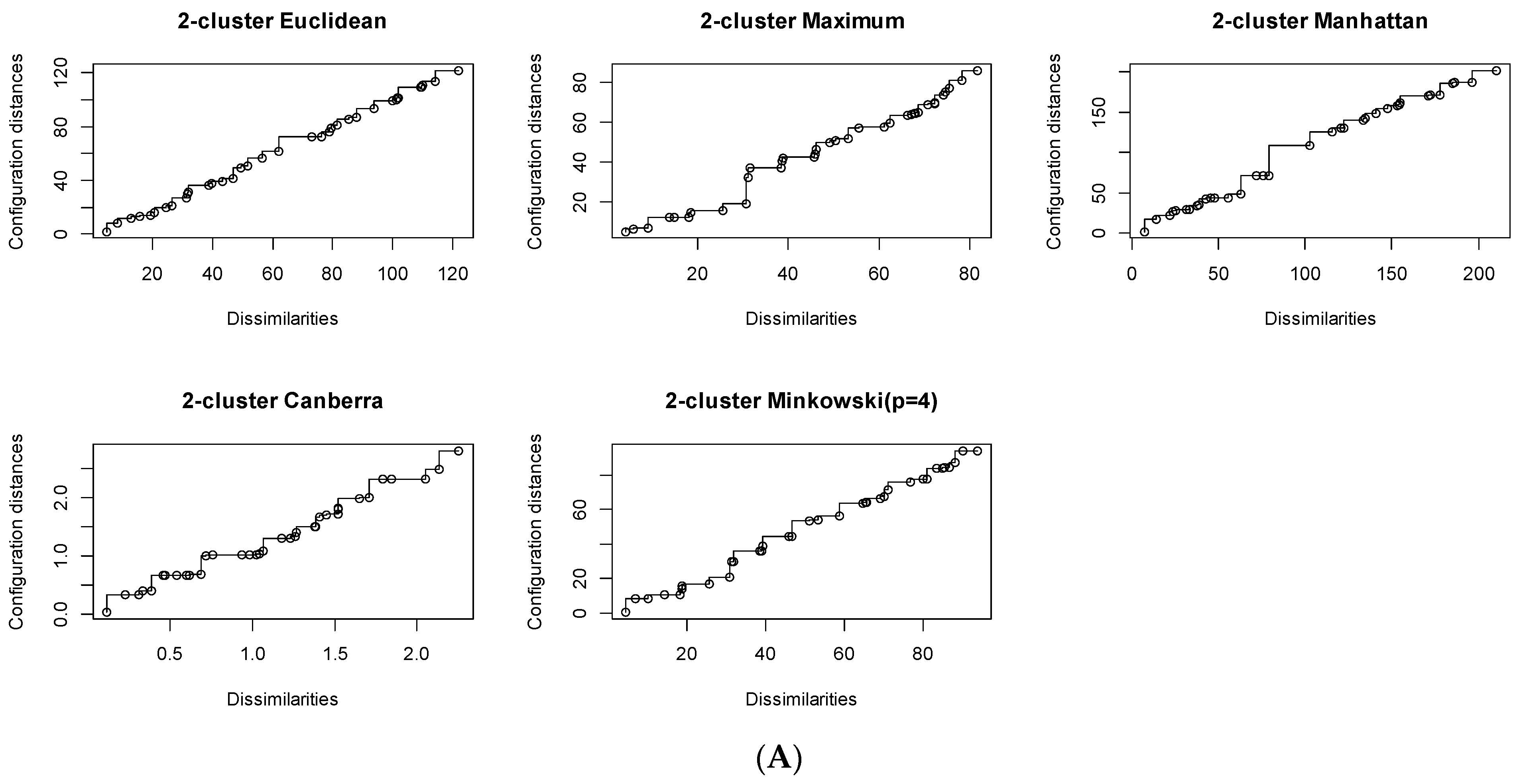
Pre-screen the number of candidate clusters by evaluating available distance measures, employing visual and numerical tools: (1) the Shepard plot and (2) the Kruskal stress estimations.

(9)

Obtain the cluster dendrogram and the Databionic-swarm-solver-labelled clusters for the reduced-response OA dataset.

(10)

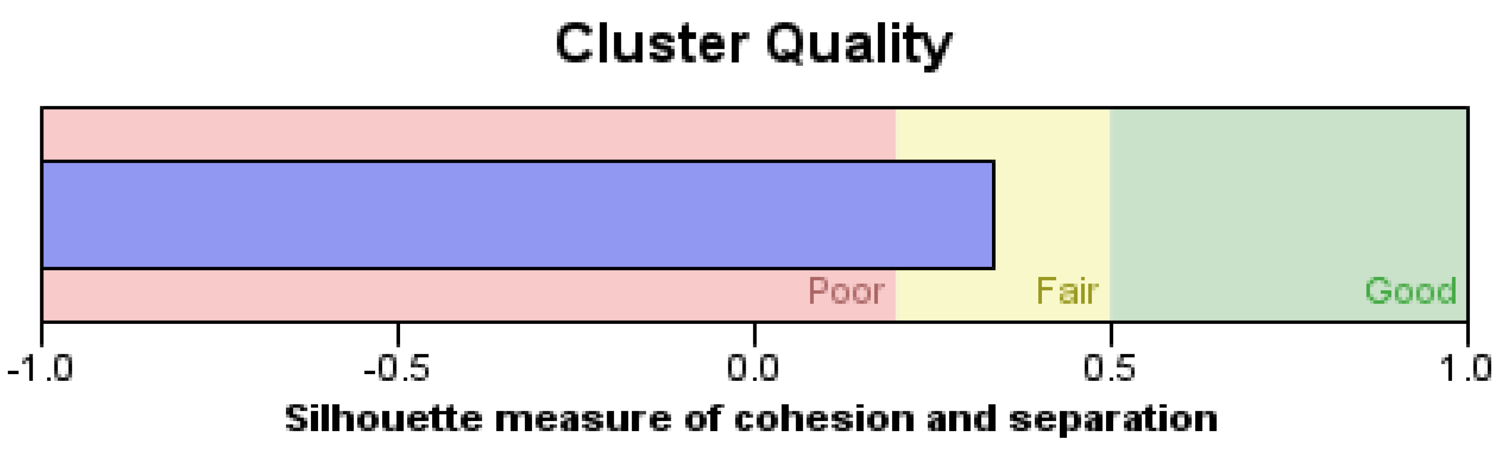
Evaluate the cluster similarity (partitioning effectiveness) between the bionic cluster-identification memberships and the pre-labelled OA factorial setting vectors by applying the Davies–Bouldin Index.

(11)

Determine the hierarchy of the potent controlling effects between the processes.

2.5. The Computational Aids

Specialized computational work was executed on the statistical freeware platform R (v. 4.3.1) [90]. The non-linear L₉(3⁴) OA array was constructed using the module ‘param.design()’ from the R-package ‘DoE.base’ (v. 1.2-2). The module ‘boxplot ()’ was used from the R-package ‘graphics’ (v. 4.3.1) to obtain robust depictions for the seven UF-membrane and the six NF-membrane process characteristics, respectively. To obtain distribution motifs, the UF/NF process characteristics were pre-screened using bean plots (R-package ‘beanplot()’ (v. 1.3.1)). The basic visual pre-screening was completed using the R-package module qqplot(). An assortment of Shepard graphs and their computed Kruskal stresses were vital in conducting the non-metric multi-dimensional scaling in order to diagnose the suitability of the five considered distance measures (‘Euclidean’, ‘maximum’, ‘Manhattan’, ‘Canberra’ or ‘Minkowski’). Thus, the respective modules ‘isoMDS()’ and ‘Shepard()’ were utilized from the R-package ‘MASS’ (v. 7.3-60). The self-organized clustering of the three UF process and the three NF process (reduced-response) mini-datasets were achieved in each case by the implementation of the Databionic swarm intelligence algorithm (R-package ‘DatabionicSwarm’ (v. 1.2.0)). The dendrogram visualization and the cluster-membership-labelled vector was created by the module ‘DBSclustering()’. To effectuate the polar stigmergic databot maneuvering, the module ‘Pswarm()’ was introduced to complete the parameter-free stochastic 2D projection mapping. The parallel distance matrix computation, using multiple threads, was facilitated by the R-package ‘parallelDist’ (v. 0.2.6). The Databionic ‘Projected-Points’ option required an intermediate distance matrix processing, which was provided by the ‘GeneratePswarmVisualization()’ module. The validation status of the cluster partitioning similarity of the two separate reduced-response mini-datasets, against the same L₉(3⁴) OA individual factorial vectors, was attained by figuring out the factorial dependencies that minimized the magnitude of Davies–Bouldin index. The module ‘index.DB()’ from the R-package ‘clusterSim’ (v. 0.51-3) was used to compute the Davies–Bouldin index.

3. Results

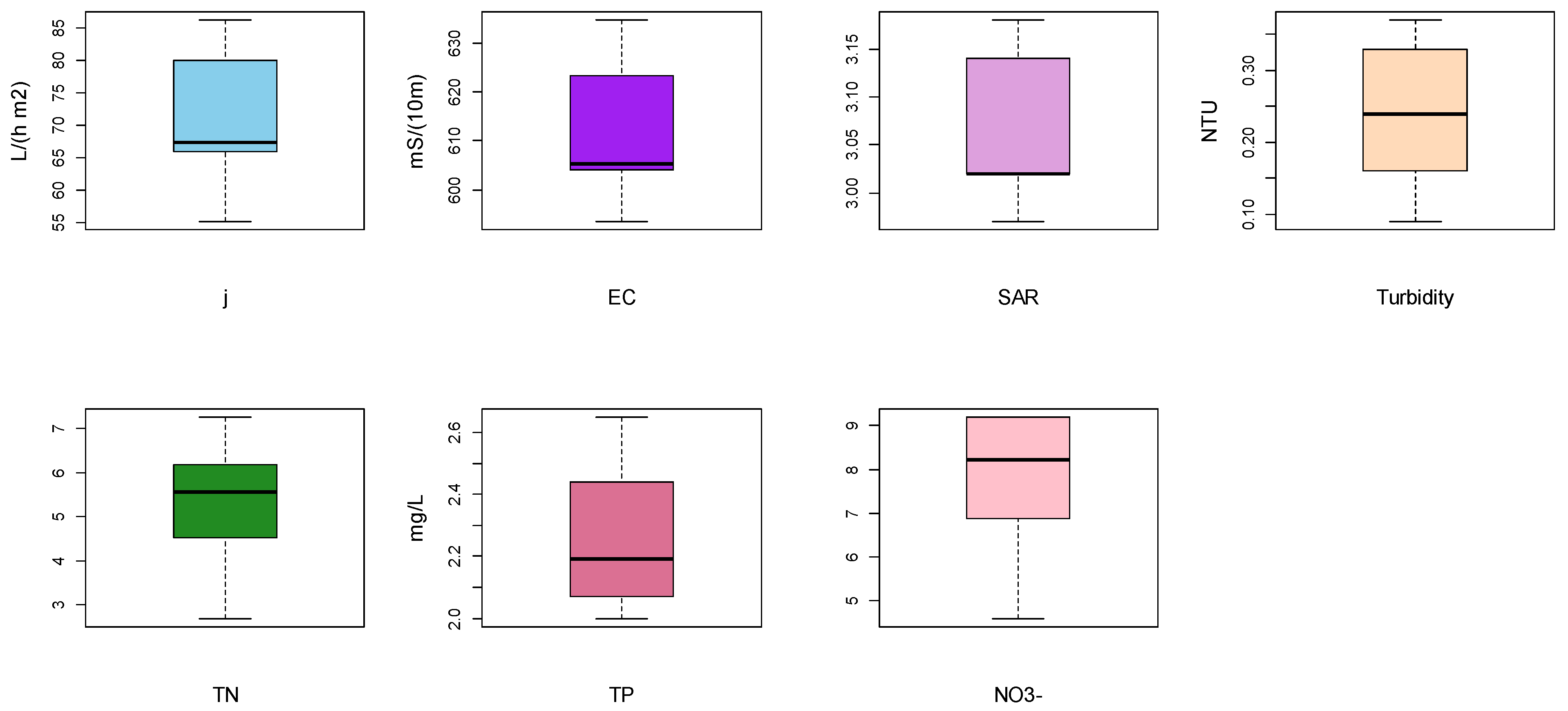
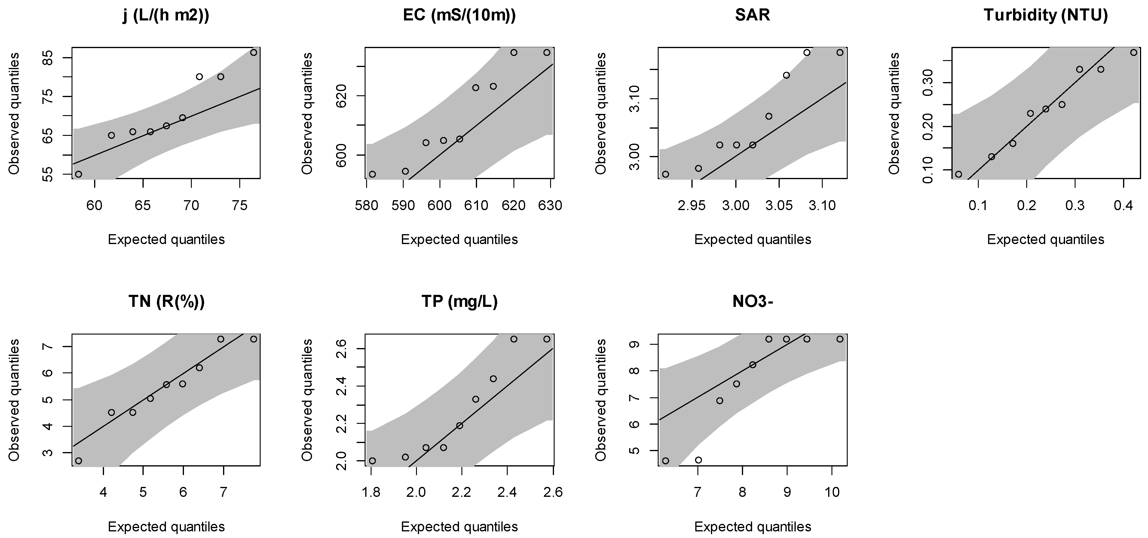
3.1. Visual Data Screening of The Multi-Characteristic Permeate Quality and Water Recovery Efficiency

3.1.1. The Ultrafiltration Process

In Figure 2, boxplot depictions of the ultrafiltration process characteristics are shown for immediate comparison. It became obvious that out of the seven responses, at least three (permeate flux, electrical conductivity and SAR) strongly deviated from a typical symmetrical distribution. It was only the turbidity data that apparently conformed to a symmetrical shape. Empirically, this implies that computing location and dispersion estimates for screening and prediction purposes might require the involvement of more sophisticated data manipulation treatments. Definitely, a second round of visual data screening using the bean plot option offered more detailed data structure properties (Figure 3). The symmetrical portrayal of the turbidity data was then more transparent. Due to the small data size, it was also noted that the total nitrogen data spread could be described by an approximate normal distribution. However, the remaining five responses exhibited diverse types of non-normal behaviors that might not even exclude bimodality; the marked data location was often situated between two discerned modes. Of course, a data screening phase may not be complete without a QQ plot presentation of the tendencies for the seven output characteristics. As shown in Figure 4, the QQ plots for the permeate flux, the SAR and the NO₃⁻ concentration responses displayed the presence of outlier points with respect to the drawn 95% confidence bands. It was noticed that the band width at the two response extremes—for all seven graphs—was marginally separated. For instance, it can be seen that for the case of the QQ plot for the permeate flux data, the two band ends could overlap, which might suggest a mild or no effect. The QQ plots for the electrical conductivity and the SAR data revealed a highly unbalanced dispersal of their respective data points around their fitted line; this was in agreement with the conclusions reached from the two previous graphical screenings.

3.1.2. The Nanofiltration Process

As shown in Figure 5, the boxplot portrayals demonstrated great differences between the behaviors of the six nanofiltration process characteristics. The permeate flux, total phosphorus and NO₃⁻ concentration measurements exhibited strong unsymmetrical data scattering, favoring either lower or higher values per case. Tendencies toward a lower permeate flux values were common with ultra- and nanofiltration trials. The datapoint groupings for the total phosphorus and the NO₃⁻ concentration measurements did not complement their behaviors in the two investigated processes. Moreover, the boxplots of the permeate flux, turbidity and total nitrogen content data were all characterized by one extreme/outlier point, which could not be overlooked given that it influenced the overall data reduction process by 11%. As shown in Figure 6, the corresponding bean plot data screening conveyed a very vivid picture of the multifaceted behavior that underscored each of the six process characteristics. Only the total nitrogen content dataset could be assumed to behave normally. The permeate flux data were definitely skewed, while the turbidity, the total phosphorus content and NO₃⁻ concentration variables appeared polarized, possibly implying a two-mode trend. A weak separation was observed among the ultrafiltration turbidity experiments (Figure 3). The two-peak disposition for the total phosphorus content was milder, as were the NO₃⁻ concentration variables in the ultrafiltration dataset. Useful information was gleaned from the QQ plot screening (Figure 7). It became transparent that the permeate flux, the total phosphorus content and the NO₃⁻ concentration variables could be affected by the occurrence of outlier/extraneous data points—contributions that collectively ranged from 33% to 56% of the total runs. In spite of the turbidity exhibiting a tight confidence band, there was an extreme data point that likely perturbed the data location and dispersion estimations. On the other hand, the electrical conductivity data possessed substantial variability, as evidenced by its consistently broader QQ plot confidence band.

3.2. Nonparametric Characteristic Correlation Estimation and Characteristic Selection on Efficiency

3.2.1. The Ultrafiltration Process

The possibility of correlation among the seven process characteristics was examined by estimating the coefficient of correlation. During the model development phase, it was instructive to identify and remove any correlated responses. According to the outcomes of the previous subsection, data normality was not guaranteed for all the investigated characteristics. In

Table 2. Confidence intervals for Spearman’s ρ correlation coefficients of the seven ultrafiltration process characteristics.

	Spearman′s Rho	Significance (Two-Tailed)	95% Confidence Intervals (Two-Tailed) a,b
			Lower	Upper
j—EC	−0.017	0.966	−0.686	0.668
j—SAR	−0.621	0.074	−0.914	0.096
j—Turb	−0.134	0.731	−0.744	0.597
j—TN	0.343	0.366	−0.435	0.828
j—TP	0.294	0.442	−0.478	0.810
j—NO3	−0.322	0.398	−0.820	0.454
EC—SAR	−0.179	0.645	−0.763	0.567
EC—Turb	0.201	0.604	−0.551	0.773
EC—TN	−0.561	0.116	−0.897	0.188
EC—TP	0.689	0.040	0.022	0.932
EC—NO3	0.252	0.512	−0.512	0.794
SAR—Turb	−0.180	0.644	−0.764	0.566
SAR—TN	−0.419	0.262	−0.854	0.361
SAR—TP	−0.262	0.496	−0.798	0.505
SAR—NO3	−0.022	0.955	−0.689	0.665
Turb—TN	−0.055	0.889	−0.706	0.646
Turb—TP	0.308	0.420	−0.466	0.815
Turb—NO3	−0.127	0.745	−0.740	0.602
TN—TP	−0.371	0.325	−0.838	0.409
TN—NO3	−0.131	0.737	−0.742	0.599
TP—NO3	0.202	0.602	−0.551	0.773

^a Estimation is based on Fisher′s r-to-z transformation. ^b Estimation of standard error is based on the formula proposed by Fieller, Hartley and Pearson.

, the confidence intervals for Spearman’s ρ correlation coefficient [91], along with its estimated significance value, are evaluated. It appeared that there was only a mediocre correlation (0.69), with a statistical significance at an error rate value of 0.05, and it was between the electrical conductivity and the total phosphorus content. The relative relationships among the seven characteristic efficiencies were quantified based on the robust estimations of the coefficient of variation—the recommended quartile coefficient of dispersion (QCD) [92]. In

Table 3. Relative importance of the seven ultrafiltration process characteristics based on the efficiency (QCD²).

Characteristics (Ultrafiltration Process)	QCD	Efficiency	Relative Efficiency	Cumulative Relative Efficiency
Turbidity	0.35	0.123	0.664	0.664
TN	0.16	0.0256	0.139	0.803
NO3	0.14	0.0196	0.106	0.909
J	0.097	0.00941	0.051	0.960
TP	0.082	0.00672	0.036	0.997
SAR	0.019	0.000361	0.002	0.999
EC	0.016	0.000256	0.001	1
	Total	0.18445	1

, it is listed as follows: (1) the QCD estimation for all the ultrafiltration process characteristics, (2) their squared values (robust version of the statistical efficiency) and (3) their cumulative relative efficiencies. It is clear that the turbidity, total nitrogen and NO₃ content led to higher inefficiencies and, hence, they contributed to the higher variabilities. The correlation of the electrical conductivity and the total phosphorous content was not further assessed since their efficiency values were small, and they were excluded from further consideration.

3.2.2. The Nanofiltration Process

As shown in

Table 4. Confidence intervals for Spearman’s ρ correlation coefficients of the six nanofiltration process characteristics.

	Spearman′s Rho	Significance (Two-Tailed)	95% Confidence Intervals (Two-Tailed) a,b
			Lower	Upper
j—EC	−0.703	0.035	−0.935	−0.049
j—Turb	−0.151	0.699	−0.751	0.586
j—TN	−0.377	0.318	−0.840	0.403
j—TP	−0.469	0.203	−0.870	0.305
j—NO3	0.468	0.204	−0.306	0.870
EC—Turb	0.500	0.170	−0.268	0.879
EC—TN	0.667	0.050	−0.019	0.926
EC—TP	0.667	0.050	−0.019	0.926
EC—NO3	−0.881	0.002	−0.976	−0.507
Turb—TN	0.217	0.576	−0.540	0.779
Turb—TP	0.333	0.381	−0.444	0.824
Turb—NO3	−0.390	0.300	−0.844	0.390
TN—TP	0.133	0.732	−0.598	0.743
TN—NO3	−0.746	0.021	−0.945	−0.139
TP—NO3	−0.339	0.372	−0.826	0.439

^a Estimation is based on Fisher′s r-to-z transformation. ^b Estimation of standard error is based on the formula proposed by Fieller, Hartley and Pearson.

, the Spearman’s ρ correlation coefficient values for the pairs (1) j-EC, (2) EC-TN, (3) EC-TP, (4) EC-NO₃ and (5) TN-NO₃ suggested that there might be a noticeable relationship between some pairs of characteristics. However, the two pairs EC-TN and EC-TP appeared to include a correlation coefficient of zero. Thus, they were removed from the five-pair group. Moreover, the pairs TN-NO₃ and j-EC included very weak (lower-bound) correlation coefficient values of −0.139 and −0.049, respectively. This made their selection doubtful, and they were removed from the initial pair screening list. It was only the Spearman’s ρ correlation coefficient value of the EC-NO₃ pair that appeared to be convincingly significant (p < 0.01). Even though the upper bound of its correlation coefficient estimate indicates a very strong negative correlation (−0.976), the lower bound of the confidence interval did not uphold the strong pairing, but it allowed the possibility for a moderate relationship (correlation coefficient value of −0.507). Thus, the next round of screening moved to the efficiency performances of the nanofiltration process characteristics (

Table 5. Relative importance of the six nanofiltration process characteristics based on the efficiency (QCD²).

Characteristics (Nanofiltration Process)	QCD	Efficiency	Relative Efficiency	Cumulative Relative Efficiency
NO3	0.614	0.377	0.389	0.389
EC	0.613	0.376	0.387	0.776
TN	0.36	0.130	0.134	0.910
J	0.24	0.0576	0.0594	0.969
TP	0.17	0.0289	0.0298	0.999
Turbidity	0.032	0.00102	0.00106	1
	Total	0.970	1

). Indeed, the electrical conductivity and the NO₃ content were comparable in generating substantial variability with respect to the other four process characteristics. The total nitrogen content joined the group of the other two characteristics to form the characteristic triplet that contributed more than 90% to the cumulative relative efficiency.

3.3. Graphical Pre-Screening of the Candidate Distance Measures

3.3.1. The Ultrafiltration Process Multi-Characteristic Distance Measure Selection

The candidate distance measures that were indicatively selected to be tested were (1) the Euclidean distance, (2) the maximum/Chebyshev distance, (3) the Manhattan distance, (4) the Canberra distance and (5) the Minkowski distance. For the Minkowski distance, the model parameter p was fitted at a value of 4. Two-cluster and three-cluster configurations were evaluated to examine the linear and non-linear dependencies on the four controlling factors. From Section 3.2.1, the participating ultrafiltration process characteristics in the clustering assignment were (1) the turbidity, (2) the total nitrogen content and (3) the NO₃ content. Shepard graphs were prepared and are contrasted in Figure 8 to provide quick visual evidence. It appeared that for both preset cluster sizes, the Euclidean distance measure provided the most satisfying representation of the relationship between the configuration distances and the dissimilarities. However, it was not easily discerned whether the two- or three-cluster setting was more accurate in delineating this behavior. Therefore, the Kruskal stress estimations for all five distance measures and the two cluster sizes are tabulated in

Table 6. Kruskal stresses pre-screening for the distance measures at two cluster number settings (ultrafiltration process characteristics).

Distance Measure	Cluster Number	Kruskal Stress Value
Euclidean	2	6.89 × 10−14
Euclidean	3	4.66 × 10−14
Maximum	2	3.13
Maximum	3	8.51 × 10−3
Manhattan	2	2.63
Manhattan	3	5.12 × 10−3
Canberra	2	9.36
Canberra	3	2.14
Minkowski (p = 4)	2	4.19 × 10−3
Minkowski (p = 4)	3	2.22 × 10−3

. Ostensibly, the three-cluster setting was favored by the fitting performances of all five distance measures. However, the best performance was witnessed for the Euclidean distance measure, since the Kruskal stress estimate was minimized at a value of 4.66 × 10⁻¹⁴. Thus, the decision was to apply the Databionic unsupervised classifier by adjusting it to utilize the Euclidean distance measure and to deliver clustering hierarchies, which were set up for a three-tier solution.

3.3.2. The Nanofiltration Process Characteristics Multi-Characteristic Distance Measure Selection

The same procedure was repeated for the nanofiltration process as in the preceding sub-section. The same five distance measures and the two cluster sizes were assessed for the nanofiltration process characteristics that were nominated from Section 3.2.2, i.e., the electrical conductivity, the NO₃ content and the total nitrogen content. The two- and three-cluster configurations of the dataset in terms of the Shepard graphs are depicted in Figure 9. While the Euclidean distance measure still provided a tighter fit between the configuration distances and the dissimilarities for the two-cluster case, the Manhattan, Canberra and Minkowski (p = 4) distance measures competed fairly well with each other. To make this distinction more accurate, the Kruskal stress estimates for all five distance measures and the two cluster sizes are tabulated in

Table 7. Kruskal stresses pre-screening for the distance measures at two-cluster number settings (nanofiltration process characteristics).

Distance Measure	Cluster Number	Kruskal Stress Value
Euclidean	2	5.42 × 10−14
Euclidean	3	6.01 × 10−14
Maximum	2	2.32 × 10−3
Maximum	3	5.15 × 10−3
Manhattan	2	9.03 ×10−3
Manhattan	3	5.58 × 10−14
Canberra	2	5.98 × 10−3
Canberra	3	6.58 × 10−14
Minkowski (p = 4)	2	7.91 × 10−3
Minkowski (p = 4)	3	5.78 × 10−14

. Again, it was observed that the three-cluster setting option led to lower Kruskal stress values for the Manhattan, Canberra and Minkowski (p = 4) distance measures. However, the minimum estimated Kruskal stress value was 5.42 × 10⁻¹⁴. It was obtained in the case of a two-cluster setting when a Euclidean distance measure was considered; it was not distinguishably different from the three-cluster size setting.

The two-cluster Euclidean-distance-measured Kruskal stress estimate was comparable to the Kruskal stress values that were obtained for the three-cluster Manhattan, Canberra and Minkowski (p = 4) distance measure models. For practical purposes, the Euclidean distance measure was retained in the tuning of the Databionic unsupervised classifier, but it was tested on both cluster sizes.

3.4. Ultrametric Self-Organizing Clustering and Validating Metric Comparison to Fractional Factorial Setting Vectors

3.4.1. The Ultrafiltration Process Parameter-Free-Projection Self-Organized Clustering

The dendrogram for the three nominated ultrafiltration process characteristics (turbidity, total nitrogen content and NO₃⁻ content) is drawn in Figure 9. The Databionic auto-classifier was propped to take advantage of the Euclidean distance metric, adjusting the position type for the projection points to complement the compact structure type, while a three-cluster model was assigned. The length of the branches was scaled on the ultrametric portion of the distance. It was observed that the first branch (runs # 1, 2) was bifolious and well separated from the rest of the runs in the L₉(3⁴) OA formulation. The second branch retained information from runs # 2–6, and the last branch was more balanced as the information was retrieved by the last three OA runs (# 7–9). To further examine the relationship of the tri-characteristic micro-dataset, the “fitting” performance was internalized. By using a popular algorithmic internal validator (the Davies–Bouldin index), the similarity evaluation process was not only restricted to quantifying a clustering effectiveness between the predicted cluster memberships and the inherent dataset. In fact, the Davies–Bouldin index could assume an extended role, i.e., that of an internal standard by which the four fractional factorial “membership” vectors were also assessed against the dataset. In

Table 8. Davies–Bouldin index estimation of ultrafiltration process tri-characteristic dataset for self-validation and fractional factorial clustering performance (p = 2, q = 1).

		Davies–Bouldin Index Estimation For Fractional Factorial Vectors
Centrotypes	Self-validation	A	B	C	D
Centroids	0.74 (0.80) *	1.89	6.79	1.88	4.7
Medoids	0.76 (1.07) *	1.27	2.08	3.55	4.44

* In parenthesis the estimation was obtained using the parameters (p = 2, q = 2).

, list the Davies–Bouldin index scores are listed for the two commonly implemented types of centrotypes: the cluster centroids and the medoids. The Davies–Bouldin Index was adjusted to the ordinary metric parameters (p, q) = (2, 1). From Table 8, it can be seen that the centroid- and medoid-based index estimations were in agreement. Additionally, the index parameter settings set at (p, q) = (2, 2) were attempted and estimated to verify that the initial (2, 1) setting offered a finer resolution of the clustering self-validation performance. There was as much as a 40% reduction in the internal validation prediction when selecting the Davies–Bouldin medoid metric, which was set at the parameter pair (2, 1) over the (2, 2) option. A corresponding difference also existed but was smaller for the centroid centrotype option. The Davies–Bouldin index estimations for the fractional factorial vectors revealed that there was a consensus in pointing at a factor that minimized the index estimate the most, and it was rather independent of the centrotype choice.

In both cases, it was the factor A (membrane type) that stood out, and its fractional factorial setting vector emulated the cluster membership vector closer to that which was derived from the Databionic classifier solution (Figure 10). Actually, the medoid metric version substantially reduced the Davies–Bouldin index estimate to a value of 1.27 with respect to the centroid-based prediction value of 1.89 (Table 8). However, there was a spilt decision on the activeness of factor C (temperature), which returned a comparable similarity prediction to factor A when the solution was based on the centroid metric, but it was not verifiable by the alternative medoid estimate. Of course, validating the micro-dataset using the medoid-mediated fractional factorial vector sequences caused the similarity index estimations to be more evenly moderated in compiling the profiled hierarchy landscape. The rest of the factors could be contemplated to be inactive. Factor A was more likely to be approximated with a linear model.

3.4.2. The Nanofiltration Process Parameter-Free Projection Self-Organized Clustering

The dendrogram for the three nominated nanofiltration process characteristics (electrical conductivity, total nitrogen content and NO₃⁻ content) is drawn in Figure 11. The Databionic classifier was adjusted to the Euclidean distance metric. The tracking of position points was carried out by projection in a compact structure. Nevertheless, two cluster sizes were examined this time, at k = 2 and 3. The length of the branches was evaluated on the ultrametric portion of the distance. The tree configuration was surprisingly identical for both of the tested cluster sizes. It was determined that there were at least two clusters that exhibited substantial differences between them. It might be said that the behavior of the data entries that were associated with runs # 1, 2 and 3 were separable from the rest of the dataset. The implementation of the Davies–Bouldin self-validator index, set at (p = 2, q = 1), greatly simplified the comparison process in four aspects in this case (

Table 9. Davies–Bouldin index estimation of nanofiltration process tri-characteristic dataset for self-validation and fractional factorial clustering performance (p = 2, q = 1).

			Davies–Bouldin Index Estimation for Fractional Factorial Vectors
Cluster Size	Centrotypes	Self-validation	A	B	C	D
k = 2	Centroids	0.39	0.41	12.1	19.97	22.87
	Medoids	0.34	0.4	5.63	5.61	5.6
k = 3	Centrotypes	Self-validation	A	B	C	D
	Centroids	0.41	0.41	12.1	19.97	22.87
	Medoids	0.4	0.4	5.63	5.61	5.6

):

(1)

The self-validation of the tri-characteristic clustering was in agreement regardless of the cluster size; the Davies–Bouldin index was confined to values between 0.34 and 0.41 for all four estimations.

(2)

The Davies–Bouldin index estimations, within a preset cluster size, was in agreement regardless of the selection of the two centrotypes. This might imply a more reliable “internal standard” with respect to the ultrafiltration process outcomes.

(3)

It was factor A that mimicked the behavior of the self-validator estimations, thus delivering the maximum information by ensuring that the similarity between the factor-A vectoring and the inherent internal clustering pattern were almost indistinguishable; the membership identification entries from the Databionic classifier and the fractional factorial setting vector for factor A matched. Particularly, for the case in which the cluster size was set at k = 3, the centroid- and medoid-based Davies–Bouldin index estimates were also identical; their computed values were 0.41 and 0.40, respectively. From this behavior, it was inferred that factor A should be assigned a simpler linear model.

(4)

The remaining three factors may be deemed weak since their Davies–Bouldin index magnitudes were substantially larger.

4. Discussion

4.1. Datacentric Evaluation by Re-Profiling Comparisons for the Ultrafiltration Process Characteristics

In discussing the outcomes of this work, it is imperative to consolidate information from grass-roots principles in data-centric engineering. A rudimentary inspection of the ultrafiltration process characteristic dataset, by standard normality tests, becomes indispensable. As long as the individual characteristic dataset is small (less than 10 measurements), the selected normality tests that are deemed appropriate for such screenings are the Shapiro–Wilk test [93] and the Kolmogorov–Smirnov test [94,95], adjusted by the Lilliefors significance (small-data) correction [96]. In

Table 10. Tests of normality for the small dataset of the seven ultrafiltration process characteristics (IBM SPSS v.29).

	Kolmogorov–Smirnov a			Shapiro–Wilk
	Statistic	Df	p-Value	Statistic	df	p-Value
J	0.208	9	0.200 *	0.927	9	0.452
EC	0.241	9	0.141	0.886	9	0.180
SAR	0.261	9	0.079	0.865	9	0.110
Turb	0.167	9	0.200 *	0.948	9	0.672
TN	0.156	9	0.200 *	0.945	9	0.633
TP	0.222	9	0.200 *	0.864	9	0.106
NO3−	0.240	9	0.142	0.800	9	0.020

* This is a lower bound of the true significance. ^a Lilliefors’s significance correction.

, the normality statistic along with the p-values are contrasted for the two tests (IBM SPSS v.29). There was a strong agreement between the two methods, suggesting that the permeate flux, the electrical conductivity, the turbidity and the total nitrogen content may obey normality. Nevertheless, there was a disagreement for the NO₃⁻ content. Under operating conditions, it might be recommended that more data would be beneficial to confidently answer any normality concerns for the remaining variates, the SAR and the total phosphorus content.

An important step in delving into the inner tendencies of a small-structured dataset is the evaluation of the measures of shape. This is because distributional shape of the data dictates the central tendency estimations, which, in turn, are paramount to ensuring accuracy in predictions in a regular DOE additive model. In

Table 11. Skewness and kurtosis with their associated standard error estimates for the seven ultra-filtration process characteristics (IBM SPSS v.29).

		PROCESS
		Ultrafiltration		Nanofiltration
Characteristic Estimator		Statistic	Std. Error	Statistic	Std. Error
J
	Skewness	0.249	0.717	1.879	0.717
	Kurtosis	−0.418	1.400	3.847	1.400
EC
	Skewness	0.251	0.717	−0.171	0.717
	Kurtosis	−1.623	1.400	−1.705	1.400
SAR
	Skewness	0.518	0.717
	Kurtosis	−1.496	1.400
TURBIDITY
	Skewness	−0.148	0.717	−2.746	0.717
	Kurtosis	−1.163	1.400	7.885	1.400
TN
	Skewness	−0.430	0.717	0.990	0.717
	Kurtosis	0.345	1.400	−0.204	1.400
TP
	Skewness	0.589	0.717	−1.023	0.717
	Kurtosis	−1.357	1.400	−0.848	1.400
NO3
	Skewness	−0.913	0.717	−0.761	0.717
	Kurtosis	−0.711	1.400	−1.720	1.400

, the skewness and the kurtosis estimates are tabulated for all seven ultrafiltration process characteristics (IBM SPSS v.29). The skewness statistic values were within the ±1 range for all of the seven examined characteristics. This implies that all characteristic location estimations may be representative owing to underlying symmetric distributions. However, the high standard error estimations quickly dismiss such assurances. It is hard to reliably preclude asymmetry in the data spread for any of the investigated characteristic. On the other hand, the permeate flux, total nitrogen content and total NO₃⁻ content were identified to a mesokurtic distribution type, but again, the standard error does not assure such assessment outcomes. Furthermore, the electrical conductivity, the SAR, the turbidity and the total phosphorus content were described by a platykurtic distribution due to high data dispersion. Unfortunately, their standard error estimates do not ascertain their level of tailedness, since a mesokurtic distribution cannot be excluded. In conclusion, the attempt to undergo an unsupervised robust clustering exercise in the Results section without imposing datacentric conditions may be justified.

By employing ordinary clustering methods like the k-means approach, the finalized cluster centers were computed; the clusters were chosen to maximize the differences among the cases in the different clusters. (

Table 12. The k-means final cluster centers (k = 3) for the seven ultrafiltration process characteristics (IBM SPSS v.29).

Characteristic	Cluster #
	1	2	3
J	62.4	68.9	83.2
EC	634.7	600.4	623.0
SAR	3.08	3.09	3.00
Turbidity	0.31	0.22	0.21
TN	3.60	5.83	6.15
TP	2.65	2.07	2.38
NO3	8.36	6.90	8.72

). Consequently, the ANOVA treatment of the k-means cluster centers gave another (descriptive) angle about how good the within-cluster groupings and their cluster center separations might fare. However, the observed significance levels were not corrected for achieving difference maximization among the cases (

Table 13. The ANOVA table for k-means cluster centers (k = 3) of the seven ultrafiltration process characteristics. (IBM SPSS v.29).

Characteristic	Cluster		Error		F-Ratio	p-Value
	Mean Square	Df	Mean Square	Df
J	232.789	2	47.418	6	4.909	0.055
EC	963.093	2	23.303	6	41.329	<0.001
SAR	0.006	2	0.007	6	0.890	0.459
Turbidity	0.006	2	0.010	6	0.587	0.585
TN	4.250	2	1.371	6	3.099	0.119
TP	0.258	2	0.005	6	55.501	<0.001
NO3	3.021	2	3.805	6	.794	0.494

). The k-means clustering result promoted the electrical conductivity and the total phosphorus content with the best partitioned properties, which was in disagreement with the outcomes of the previous section. However, the IBM SPSS (v.29) Statistics two-step cluster analysis rated the overall quality of the clustering effort at least as fair (k = 3) by using the silhouette measure to size the dissimilarities among the clusters (Figure 12). Evidently, this seven-characteristic dataset has an innate clusterability before attempting to refine it by eliminating a portion of the process characteristics as mere “noise” responses.

To test the clusterability of the Databionic swarm classifier in a practical manner, the mean silhouette was estimated and plotted by cluster (Figure 13). Each cluster was compared against the next best cluster for dissimilarity using the Euclidean measure (IBM SPSS v.29). The Databionic swarm solution involves only the three nominated process characteristics, as explained in the previous section. It is obvious that cluster #3 achieved greater separability first with respect to cluster #2 and then with cluster #1. It may be concluded that the Databionic micro-clustering effort can be regarded as satisfactory. In Figure 14, the four factors are individually self-contrasted. It was observed that only for factor A (membrane type), a mean silhouette measure estimate was worth considering, and it declared the membrane type as an active influence; a mean silhouette value close to 0.5 was obtained (Figure 14A). A greater separation was identified between factorial levels #1 and #2, which denotes that the emergent stigmergic search tended to match the clustering solution to the factorial run order for factor A, as dictated by the L₉(3⁴) OA scheme.

4.2. Datacentric Evaluation by Re-Profiling Comparisons for the Nanofiltration Process Characteristics

Repeating the same procedure for the basic normality screening of the nanofiltration process characteristics, the Shapiro–Wilk test and the Kolmogorov–Smirnov test results (adjusted by the Lilliefors significance correction) for the six characteristics are listed in

Table 14. Tests of normality for the small dataset of the six nanofiltration process characteristics (IBM SPSS v.29).

Characteristic	Kolmogorov–Smirnov a			Shapiro–Wilk
	Statistic	Df	p-Value	Statistic	Df	p-Value
J	0.283	9	0.036	0.735	9	0.004
EC	0.198	9	0.200*	0.888	9	0.192
Turbidity	0.376	9	<0.001	0.597	9	<0.001
TN	0.247	9	0.121	0.872	9	0.131
TP	0.345	9	0.003	0.761	9	0.007
NO3−	0.291	9	0.027	0.731	9	0.003

* This is a lower bound of the true significance. ^a Lilliefors’s significance correction.

. There was strong agreement between the two methods; however, the Shapiro–Wilk test gave finer statistical significance values at an error rate of 0.05. Normality was not assured for four of the characteristics: (1) the permeate flux, (2) the turbidity, (3) the total phosphorus content and (4) the NO₃⁻ concentration. Under operating conditions, the total nitrogen content could be also monitored more closely.

Next, the respective measures of shape were computed for the six nanofiltration process characteristics, which are listed in Table 11. The skewness estimations for the permeate flux, the turbidity and the total phosphorus content exceeded the ±1 range, trending on either direction; the permeate flux sample distribution was right-tailed, while the turbidity and total phosphorus content were left-tailed. This may imply that skewness was a suspected contributor to the diagnosed non-normality for the three characteristics. The rest of the characteristics were not protected from manifesting deviant non-normal behaviors, as was suggested by their computed high standard error values. Additionally, platykurtic sample distributions were identified with the electrical conductance and the NO₃⁻ concentration data. The permeate flux and turbidity sample distributions appeared leptokurtic. The remaining two characteristic sample distributions may appear mesokurtic; nevertheless, the high values of the standard error estimations do not permit a terminal tailedness classification rating. Finally, excessive kurtosis may also be a justification for the observed deviations from normality due to the data outliers.

To test the clusterability of the Databionic swarm classifier in a practical manner, the mean-silhouette-by-cluster bar chart is drawn in Figure 15 for a cluster size set at k = 3. Each cluster was compared against the next best cluster for dissimilarity using the Euclidean measure (IBM SPSS v.29). The Databionic swarm solution involved only the three nominated nanofiltration process characteristics: (1) the electrical conductivity, (2) the total nitrogen content and (3) the NO₃ content (Section 3.2.2). It is obvious that clusters #1 and #2 rendered cluster #3 as the next best cluster. It may be concluded that the Databionic micro-clustering effort can be regarded as satisfactory, regardless of the preference of initiating the clustering process through either cluster #1 or #2. The direct relationship between fractional factorial vectoring and emergent stigmergic clustering is shown in Figure 16, where all four controlling factors are individually self-contrasted. As in the screening of the nominated ultrafiltration process characteristics, it was discovered that only factor A (membrane type) posted a high mean silhouette measure estimation (Figure 16A). OA factorial data # 1 and #2 generated a substantial separation with factorial cluster #3, which was supported by a mean silhouette value larger than 0.8 for both clustered groups. In other words, the bionic clustering solution closely matched the factorial run order for factor A, as dictated by the L₉(3⁴) OA scheme. In Figure 17, it is confirmed that there was a detectable separation between clusters #2 and #1, which was viable even when a clustering size of k = 2 was selected. It seems a linear relationship may associate the membrane type influence with the triplet nanofiltration process characteristics.

5. Conclusions

As water resources are rendered scarce, ultrafiltration (UF) and nanofiltration (NF) membranes facilitate the development of sustainable separation solutions. Moreover, there are lean-and-green incentives for single-stage filtration processes in treating urban wastewater. The screening and optimization of single-stage UF-/NF-membrane wastewater processes require the tailored design of the operations by taking in account several aspects that range from customization of the treatment unit to the condition of the incoming wastewater volumes as well as the functionality of the selected membranes in specific operating conditions, namely the mass transfer properties and solute rejection. In realistic circumstances, process customization success is subject to a holistic comprehension of the separation dynamics that involve selected structural membrane properties and their physicochemical interactions with the wastewater medium. Taguchi-type methods may be employed for quick and economical studies that intend to improve the filtration performance for a single process characteristic. However, to screen and optimize physicochemical separation processes, Taguchi-type orthogonal array sampling recipes are still useful in generating small multi-characteristic non-linear datasets, even when the collected responses are described by different measurement scales and data types. In spite of the availability of various statistical multivariate techniques to handle the multifactorial multi-response problem, there is a great interest for unsupervised algorithmic solvers.

The approach that was tested in this work attempted to firstly cluster the gathered multi-response dataset and then try to directly match the stochastic signature of the clustered members to the factorial vector sequences in the orthogonal array in a naïve backtracking exercise. The technique was applied on recently published multi-characteristic multifactorial data for a single-stage urban wastewater operation that involved as many as seven UF-membrane process characteristics and six NF-membrane process characteristics. The investigated controlling factors were the (1) membrane type, (2) cross-flow velocity, (3) temperature and (4) transmembrane pressure. The data analysis part was inherently demanding because the generated dataset was constructed based on the restrictive Taguchi-type L₉(3⁴) OA; the factorial screening, effect curvatures and parameter optimization were expected to be explained by only nine observations per process characteristic. The Databionic swarm intelligence classifier was implemented to complete the cluster identification task. Minimization of the Davies–Bouldin similarity measure revealed the more influential controlling factors by contrasting the appropriateness of the configuration of the cluster identification vector to the factorial-setting vector pattern. It was found that the membrane type in both filtration setups was the controlling factor that predominantly influenced their respective groups of the UF-/NF-membrane process characteristics. Future work could reconcile the bionic solver predictions of the two processes by making use of unsupervised stochastic comparison treatments.

References

1. United Nations. Sustainable Development Goals, Goal 6: Clean Water and Sanitation. Available online: https://www.undp.org/sustainable-development-goals/clean-water-and-sanitation (accessed on 21 September 2023).
2. Mekonnen, M.M.; Hoekstra, A.Y. Four billion people facing severe water scarcity. Sci. Adv. 2016, 2, e1500323. [Google Scholar] [CrossRef] [PubMed]
3. Kummu, M.; Guillaume, J.H.A.; de Moel, H.; Eisner, S.; Florke, M.; Porkka, M.; Siebert, S.; Veldkamp, T.I.E.; Ward, P.J. The world’s road to water scarcity: Shortage and stress in the 20th century and pathways towards sustainability. Sci. Rep. 2016, 6, 38495. [Google Scholar] [CrossRef] [PubMed]
4. Liu, J.; Yang, H.; Gosling, S.N.; Kummu, M.; Florke, M.; Pfister, S.; Hanasaki, N.; Wada, Y.; Zhang, X.; Zheng, C.; et al. Water scarcity assessments in the past, present, and future. Earths Future 2017, 5, 545–559. [Google Scholar] [CrossRef] [PubMed]
5. ISO 14046; Environmental Management-Water Footprint-Principles, Requirements and Guidelines. International Organization for Standardization: Geneva, Switzerland, 2014.
6. Hoekstra, A.Y.; Mekonnen, M.M. The water footprint of humanity. Proc. Natl. Acad. Sci. USA 2012, 109, 3232–3237. [Google Scholar] [CrossRef] [PubMed]
7. Vanham, D.; Hoekstra, A.Y.; Wada, Y.; Bouraoui, F.; de Roo, A.; Mekonnen, M.M.; van de Bund, W.J.; Batelan, O.; Pavelic, P.; Bastiaanssen, W.G.M.; et al. Physical water scarcity metrics for monitoring progress towards SDG target 6.4: An evaluation of indicator 6.4.2 “Level of water stress”. Sci. Total Environ. 2018, 613–614, 218–232. [Google Scholar] [CrossRef] [PubMed]
8. Zeng, Z.; Liu, J.; Savenije, H.H.G. A simple approach to assess water scarcity integrating water quantity and quality. Econ. Indic. 2013, 34, 441–449. [Google Scholar] [CrossRef]
9. Liu, J.; Liu, Q.; Yang, H. Assessing water scarcity by simultaneously considering environmental flow requirements, water quantity, and water quality. Ecol. Indic. 2016, 60, 434–441. [Google Scholar] [CrossRef]
10. Quinteiro, P.; Ridoutt, B.G.; Arroja, L.; Dias, A.C. Identification of methodological challenges remaining in the assessment of a water scarcity footprint: A review. Int. J. Life Cycle Assess. 2018, 23, 164–180. [Google Scholar] [CrossRef]
11. Schuns, J.F.; Hoekstra, A.Y.; Booij, M.J. Review and classification of indicators of green water availability and scarcity. Hydrol. Earth Syst. Sci. 2015, 12, 5519–5564. [Google Scholar] [CrossRef]
12. Kahil, T.; Albiac, J.; Fischer, G.; Strokal, M.; Tramberend, S.; Greve, P.; Tang, T.; Burek, P.; Burtscher, R.; Wada, Y. A nexus modeling framework for assessing water scarcity solutions. Curr. Opin. Environ. Sustain. 2019, 40, 72–80. [Google Scholar] [CrossRef]
13. Ledari, M.B.; Saboohi, Y.; Azamian, S. Water-food-energy-ecosystem nexus model development: Resource scarcity and regional development. Energy Nexus 2023, 10, 100207. [Google Scholar] [CrossRef]
14. Shemer, H.; Wald, S.; Semiat, R. Challenges and Solutions for Global Water Scarcity. Membranes 2023, 13, 612. [Google Scholar] [CrossRef] [PubMed]
15. Wu, C.; Liu, W.; Deng, H. Urbanization and the Emerging Water Crisis: Identifying Water Scarcity and Environmental Risk with Multiple Applications in Urban Agglomerations in Western China. Sustainability 2023, 15, 12977. [Google Scholar] [CrossRef]
16. Pierrat, E.; Laurent, A.; Dorber, M.; Rygaard, M.; Verones, F.; Hauschild, M. Advancing water footprint assessments: Combining the impacts of water pollution and scarcity. Sci. Total Environ. 2023, 870, 161910. [Google Scholar] [CrossRef] [PubMed]
17. Li, H.; Chen, Q.; Liu, G.; Lombardi, G.V.; Su, M.; Yang, Z. Uncovering the risk spillover of agricultural water scarcity by simultaneously considering water quality and quantity. J. Environ. Manag. 2023, 343, 118209. [Google Scholar] [CrossRef] [PubMed]
18. Mekonnen, M.M.; Hoekstra, A.Y. The green, blue and grey water footprint of crops and derived crop products. Hydrol. Earth Syst. Sci. 2011, 15, 1577–1600. [Google Scholar] [CrossRef]
19. Mancosu, N.; Snyder, R.L.; Kyriakakis, G.; Spano, D. Water scarcity and future challenges for food production. Water 2015, 7, 975–992. [Google Scholar] [CrossRef]
20. Winter, J.M.; Lopez, J.R.; Ruane, A.C.; Young, C.A.; Scanlon, B.R.; Rosenzweig, C. Representing water scarcity in future agricultural assessments. Anthropocene 2017, 18, 15–26. [Google Scholar] [CrossRef]
21. Ingrao, C.; Strippoli, R.; Lagioia, G.; Huisingh, D. Water scarcity in agriculture: An overview of causes, impacts and approaches for reducing the risks. Heliyon 2023, 9, e18507. [Google Scholar] [CrossRef] [PubMed]
22. Morante-Carballo, F.; Montalván-Burbano, N.; Quiñonez-Barzola, X.; Jaya-Montalvo, M.; Carrión-Mero, P. What do We Know about Water Scarcity in Semi-Arid Zones? A Global Analysis and Research Trends. Water 2022, 14, 2685. [Google Scholar] [CrossRef]
23. Ungureanu, N.; Vladut, V.; Voicu, G. Water scarcity and wastewater reuse in crop irrigation. Sustainability 2020, 12, 9055. [Google Scholar] [CrossRef]
24. Jaramillo, M.F.; Restrepo, I. Wastewater reuse in agriculture: A review about its limitations and benefits. Sustainability 2017, 9, 1734. [Google Scholar] [CrossRef]
25. Lopez-Serrano, M.J.; Velasco-Munoz, J.F.; Arnar-Sanchez, J.A.; Roman-Sanchez, I.M. Sustainable use of wastewater in agriculture: A bibliometric analysis of worldwide research. Sustainability 2020, 12, 8948. [Google Scholar] [CrossRef]
26. Elgallal, M.; Fletcher, L.; Evans, B. Assessment of potential risks associated with chemicals in wastewater used for irrigation in arid and semiarid zones: A review. Agr. Water Manag. 2016, 177, 419–431. [Google Scholar] [CrossRef]
27. Saliu, T.D.; Oladoja, N.A. Nutrient recovery from wastewater and reuse in agriculture: A review. Environ. Chem. Lett. 2021, 19, 2299–2316. [Google Scholar] [CrossRef]
28. Gude, V.G. Desalination and water reuse to address global water scarcity. Rev. Environ. Sci. Biotechnol. 2017, 16, 591–609. [Google Scholar] [CrossRef]
29. Jimenez, S.; Mico, M.M.; Arnaldos, M.; Medina, F.; Contreras, S. State of the art of produced water treatment. Chemosphere 2018, 192, 186–208. [Google Scholar] [CrossRef]
30. Younas, F.; Mustafa, A.; Rahman Farooqi, Z.U.; Wang, X.; Younas, S.; Mohy-Ud-Din, W.; Hameed, M.A.; Abrar, M.M.; Maitlo, A.A.; Noreen, S.; et al. Current and emerging adsorbent technologies for wastewater treatment: Trends, limitations, and environmental implications. Water 2021, 13, 215. [Google Scholar] [CrossRef]
31. Davis, M. Water and Wastewater Engineering: Design Principles and Practice; McGraw Hill: New York, NY, USA, 2019. [Google Scholar]
32. Edzwald, J. Water Quality and Treatment: A Handbook on Drinking Water; McGraw Hill: New York, NY, USA, 2010. [Google Scholar]
33. Mohammad, A.W.; Teow, Y.H.; Ang, W.L.; Chung, Y.T.; Oatley-Radcliffe, D.L.; Hilal, N. Nanofiltration membranes review: Recent advances and future prospects. Desalination 2015, 356, 226–254. [Google Scholar] [CrossRef]
34. Jia, T.-Z.; Rong, M.-Y.; Chen, C.-T.; Yong, W.F.; Lau, S.K.; Zhou, R.F.; Chen, M.; Sun, S.P. Recent advances in nanofiltration-based hybrid processes. Desalination 2023, 565, 116852. [Google Scholar] [CrossRef]
35. Rabiee, N.; Sharma, R.; Foorginezhad, S.; Jouyandeh, M.; Asadnia, M.; Rabiee, M.; Akhavan, O.; Lima, E.C.; Formela, K.; Ashrafizadeh, M.; et al. Green and Sustainable Membranes: A review. Environ. Res. 2023, 231, 116133. [Google Scholar] [CrossRef]
36. Elsaid, K.; Olabi, A.G.; Abdel-Wahab, A.; Elkamel, A.; Alami, A.H.; Inayat, A.; Chae, K.-J.; Abdelkareem, M.A. Membrane processes for environmental remediation of nanomaterials: Potentials and challenges. Sci. Total Environ. 2023, 879, 162569. [Google Scholar] [CrossRef] [PubMed]
37. Fu, F.; Wang, Q. Removal of heavy metal ions from wastewaters: A review. J. Environ. Manag. 2011, 92, 407–418. [Google Scholar] [CrossRef] [PubMed]
38. Parashar, N.; Hait, S. Recent advances on microplastics pollution and removal from wastewater systems: A critical review. J. Environ. Manag. 2023, 340, 118014. [Google Scholar] [CrossRef] [PubMed]
39. Kima, S.; Chua, K.H.; Al-Hamadania, Y.A.J.; Park, C.M.; Jang, M.; Kim, D.-H.; Yue, M.; Heof, J.; Yoon, Y. Removal of contaminants of emerging concern by membranes in water and wastewater: A review. Chem. Eng. J. 2018, 335, 896–914. [Google Scholar] [CrossRef]
40. Alzahrania, S.; Mohammad, A.W. Challenges and trends in membrane technology implementation for produced water treatment: A review. J. Water Process Eng. 2014, 4, 107–133. [Google Scholar] [CrossRef]
41. Al Aania, S.; Mustafa, T.N.; Hilal, N. Ultrafiltration membranes for wastewater and water process engineering: A comprehensive statistical review over the past decade. J. Water Process Eng. 2020, 35, 101241. [Google Scholar] [CrossRef]
42. Ji, K.; Liu, C.; He, H.; Mao, X.; Wei, L.; Wang, H.; Zhang, M.; Shen, Y.; Sun, R.; Zhou, F. Research Progress of Water Treatment Technology Based on Nanofiber Membranes. Polymers 2023, 15, 741. [Google Scholar] [CrossRef] [PubMed]
43. Zhao, Y.; Tong, T.; Wang, X.; Lin, S.; Reid, E.M.; Chen, Y. Differentiating Solutes with Precise Nanofiltration for Next Generation Environmental Separations: A Review. Environ. Sci. Technol. 2021, 55, 1359–1376. [Google Scholar] [CrossRef] [PubMed]
44. Qiu, Y.; Depuydt, S.; Ren, L.-F.; Zhong, C.; Wu, C.; Shao, J.; Xia, L.; Zhao, Y.; Van der Bruggen, B. Progress of Ultrafiltration-Based Technology in Ion Removal and Recovery: Enhanced Membranes and Integrated Processes. ACS EST Water 2023, 3, 1702–1719. [Google Scholar] [CrossRef]
45. Zhao, M.; Xu, Y.; Zhang, C.; Rong, H.; Zeng, G. New trends in removing heavy metals from wastewater. Appl. Microbiol. Biotechnol. 2016, 100, 6509–6518. [Google Scholar] [CrossRef]
46. Kaswan, M.S.; Rathi, R.; Cross, J.; Garza-Reyes, J.A.; Antony, J.; Yadav, V. Integrating Green Lean Six Sigma and industry 4.0: A conceptual framework. J. Manuf. Technol. Manag. 2023, 34, 87–121. [Google Scholar] [CrossRef]
47. Rajarajeswari, C.; Anbalagan, C. Integration of the green and lean principles for more sustainable development: A case study. Mater. Today Proc. 2023; in press. [Google Scholar] [CrossRef]
48. Yadav, Y.; Kaswan, M.S.; Gahlot, P.; Duhan, R.K.; Garza-Reyes, J.A.; Rathi, R.; Chaudhary, R.; Yadav, G. Green Lean Six Sigma for sustainability improvement: A systematic review and future research agenda. Int. J. Lean Six Sigma 2023, 14, 759–790. [Google Scholar] [CrossRef]
49. Yadav, S.; Samadhiya, A.; Kumar, A.; Majumdar, A.; Garza-Reyes, J.A.; Luthra, S. Achieving the sustainable development goals through net zero emissions: Innovation-driven strategies for transitioning from incremental to radical lean, green and digital technologies. Resour. Conserv. Recycl. 2023, 197, 107094. [Google Scholar] [CrossRef]
50. Fiorello, M.; Gladysz, B.; Corti, D.; Wybraniak-Kujawa, M.; Ejsmont, K.; Sorlini, M. Towards a smart lean green production paradigm to improve operational performance. J. Clean. Prod. 2023, 413, 137418. [Google Scholar] [CrossRef]
51. Elemure, I.; Dhakal, H.N.; Leseure, M.; Radulovic, J. Integration of Lean Green and Sustainability in Manufacturing: A Review on Current State and Future Perspectives. Sustainability 2023, 15, 10261. [Google Scholar] [CrossRef]
52. Vinuesa, R.; Azizpour, H.; Leite, I.; Balaam, M.; Dignum, V.; Domisch, S.; Fellander, A.; Langhans, S.D.; Tegmark, M.; Nerini, F.F. The role of artificial intelligence in achieving the Sustainable Development Goals. Nature Commun. 2020, 11, 233. [Google Scholar] [CrossRef] [PubMed]
53. Farrukh, A.; Mathrani, S.; Sajjad, A. Green-lean-six sigma practices and supporting factors for transitioning towards circular economy: A natural resource and intellectual capital-based view. Resour. Policy 2023, 84, 103789. [Google Scholar] [CrossRef]
54. Kaswan, M.S.; Rathi, R.; Garza-Reyes, J.A.; Antony, J. Green Lean Six Sigma sustainability—Oriented project selection and implementation framework for manufacturing industry. Int. J. Lean Six Sigma 2023, 14, 33–71. [Google Scholar] [CrossRef]
55. Fercoq, A.; Lamouri, S.; Carbone, V. Lean/Green integration focused on waste reduction techniques. J. Clean. Prod. 2016, 137, 567–578. [Google Scholar] [CrossRef]
56. Dieste, M.; Panizzolo, R.; Garza-Reyes, J.A.; Anosike, A. The relationship between lean and environmental performance: Practices and measures. J. Clean. Prod. 2019, 224, 120–131. [Google Scholar] [CrossRef]
57. George, M.; Blackwell, D.; Rajan, D. Lean Six Sigma in the Age of Artificial Intelligence: Harnessing the Power of the Fourth Industrial Revolution; McGraw-Hill: New York, NY, USA, 2019. [Google Scholar]
58. George, M.; Works, J.; Watson-Hemphill, K. Fast Innovation: Achieving Superior Differentiation, Speed to Market, and Increased Profitability; McGraw-Hill: New York, NY, USA, 2005. [Google Scholar]
59. Bolisetty, S.; Peydayesh, M.; Mezzenga, R. Sustainable technologies for water purification from heavy metals: Review and analysis. Chem. Soc. Rev. 2019, 48, 463–487. [Google Scholar] [CrossRef] [PubMed]
60. Wang, K.; Wang, X.; Januszewski, B.; Liu, Y.; Li, D.; Fu, R.; Elimelech, M.; Huang, X. Tailored design of nanofiltration membranes for water treatment based on synthesis–property–performance relationships. Chem. Soc. Rev. 2022, 51, 672–719. [Google Scholar] [CrossRef] [PubMed]
61. Burn, D.H.; McBean, E.A. Optimization modelling of water quality in an uncertain environment. Water Resour. Res. 1985, 21, 934–940. [Google Scholar] [CrossRef]
62. Yasar, A.; Dogan, E.C.; Ayberk, H.S.; Aydiner, C. Water Recovery from Urban Wastewater for Irrigation using Ultrafiltration and Nanofiltration: Optimization and Performance. Clean Soil Air Water 2022, 50, 2200280. [Google Scholar] [CrossRef]
63. Malviya, A.; Jaspal, D. Artificial intelligence as an upcoming technology in wastewater treatment: A comprehensive review. Environ. Technol. Rev. 2021, 10, 177–187. [Google Scholar] [CrossRef]
64. Pilar Callao, M. Multivariate experimental design in environmental analysis. Trends Anal. Chem. 2014, 62, 86–92. [Google Scholar] [CrossRef]
65. Fisher, R.A. Statistical Methods, Experimental Design, and Scientific Inference; Oxford University Press: Oxford, UK, 1990. [Google Scholar]
66. Box, G.E.P.; Hunter, W.G.; Hunter, J.S. Statistics for Experimenters—Design, Innovation, and Discovery; Wiley: New York, NY, USA, 2005. [Google Scholar]
67. Taguchi, G.; Chowdhury, S.; Wu, Y. Quality Engineering Handbook; Wiley: Hoboken, NJ, USA, 2004. [Google Scholar]
68. Taguchi, G.; Chowdhury, S.; Taguchi, S. Robust Engineering: Learn How to Boost Quality while Reducing Costs and Time to Market; McGraw-Hill: New York, NY, USA, 2000. [Google Scholar]
69. Perrett, J.J.; Higgins, J.J. A Method for Analyzing Unreplicated Agricultural Experiments. Crop Sci. 2006, 46, 2482–2485. [Google Scholar] [CrossRef]
70. Stewart-Oaten, A.; Bence, J.R.; Osenberg, C.W. Assessing effects of unreplicated perturbations: No simple solutions. Ecology 1992, 73, 1396. [Google Scholar] [CrossRef]
71. Pagliari, P.H.; Ranaivoson, A.Z.; Strock, J.S. Options for statistical analysis of unreplicated paired design drainage experiments. Agr. Water Manag. 2021, 244, 106604. [Google Scholar] [CrossRef]
72. Hamada, M.; Balakrishnan, N. Analyzing unreplicated factorial experiments: A review with some new proposals. Stat. Sin. 1998, 8, 1–28. [Google Scholar]
73. Derringer, G.; Suich, R. Simultaneous optimization of several response variables. J. Qual. Technol. 1980, 12, 214–219. [Google Scholar] [CrossRef]
74. Carlson, R.; Nordahl, A.; Barth, T.; Myklebust, R. An approach to evaluating screening experiments when several responses are measured. Chemom. Intell. Lab. Syst. 1991, 12, 237–255. [Google Scholar] [CrossRef]
75. Nicolis, G.; Prigogine, I. Self-Organization in Nonequilibrium Systems: From Dissipative Structures to Order through Fluctuations; Wiley: Hoboken, NJ, USA, 1977. [Google Scholar]
76. Prigogine, I. The End of Certainty; Free Press: New York, NY, USA, 1997. [Google Scholar]
77. Breiman, L. Statistical modeling: The two cultures. Stat. Sci. 2001, 16, 199–231. [Google Scholar] [CrossRef]
78. Besseris, G.J. Concurrent multiresponse multifactorial screening of an electrodialysis process of polluted wastewater using robust non-linear Taguchi profiling. Chemom. Intell. Lab. Syst. 2020, 200, 103997. [Google Scholar] [CrossRef]
79. Besseris, G. Micro-Clustering and Rank-Learning Profiling of a Small Water-Quality Multi-Index Dataset to Improve a Recycling Process. Water 2021, 13, 2469. [Google Scholar] [CrossRef]
80. Besseris, G. Wastewater Quality Screening Using Affinity Propagation Clustering and Entropic Methods for Small Saturated Nonlinear Orthogonal Datasets. Water 2022, 14, 1238. [Google Scholar] [CrossRef]
81. Thrun, M.C.; Ultsch, A. Swarm intelligence for self-organized clustering. Artif. Intell. 2021, 290, 103237. [Google Scholar] [CrossRef]
82. Thrun, M.C. Projection-Based Clustering through Self-Organization and Swarm Intelligence; Springer: Berlin/Heidelberg, Germany, 2018; ISBN 978-3658205393. [Google Scholar]
83. Shepard, R.N. The analysis of proximities: Multidimensional scaling with an unknown distance function-Part II. Psychometrika 1962, 27, 219–246. [Google Scholar] [CrossRef]
84. Kruskal, J.B. Multidimensional scaling by optimizing goodness of fit to a nonmetric hypothesis. Psychometrika 1964, 29, 1–27. [Google Scholar] [CrossRef]
85. Davies, D.L.; Bouldin, D.W. A cluster separation measure. IEEE Trans. Pattern Anal. Mach. Intell. 1979, 1, 224–227. [Google Scholar] [CrossRef]
86. Nash, J. Non-cooperative games. Ann. Math. 1951, 54, 286–295. [Google Scholar] [CrossRef]
87. McGill, R.; Tukey, J.W.; Larsen, W.A. Variations of box plots. Am. Stat. 1978, 32, 12–16. [Google Scholar]
88. Wilk, M.B.; Gnanadesikan, R. Probability plotting methods for the analysis of data. Biometrika 1968, 55, 1–17. [Google Scholar] [CrossRef] [PubMed]
89. Kampstra, P. Beanplot: A boxplot alternative for visual comparison of distributions. J. Stat. Soft. 2008, 28, 1–9. [Google Scholar] [CrossRef]
90. R Core Team. R (Version 4.3.1): A Language and Environment for Statistical Computing; R Foundation for Statistical Computing: Vienna, Austria, 2023; Available online: https://www.R-project.org/ (accessed on 16 June 2023).
91. Spearman, C. The proof and measurement of association between two things. Am. J. Psych. 1904, 15, 72–101. [Google Scholar] [CrossRef]
92. Zwillinger, D.; Kokoska, S. Standard Probability and Statistical Tables and Formula; Chapman & Hall: Boca Raton, FL, USA, 2000. [Google Scholar]
93. Shapiro, S.S.; Wilk, M.B. An analysis of variance test for normality (complete samples). Biometrika 1965, 52, 591–611. [Google Scholar] [CrossRef]
94. Kolmogorov, A. Sulla determinazione empirica di una legge di distibuzione. Giorn. Ist. Ital. Attuari 1933, 4, 83–91. [Google Scholar]
95. Smirnov, N. Table for estimating the goodness of fit of empirical distributions. Ann. Math. Stat. 1948, 19, 279–281. [Google Scholar] [CrossRef]
96. Lilliefors, H.W. On the Kolmogorov-Smirnov test for normality with mean and variance unknown. J. Am. Stat. Assoc. 1967, 62, 399–402. [Google Scholar] [CrossRef]
Figure 1. Factorial input cluster output similarity matching process.
Applsci 13 11926 g001
Figure 2. Boxplot screening of the seven ultrafiltration process characteristics.
Applsci 13 11926 g002
Figure 3. Bean plot screening of the seven ultrafiltration process characteristics.
Applsci 13 11926 g003
Figure 4. QQ plot screening of the seven ultrafiltration process characteristics.
Applsci 13 11926 g004
Figure 5. Boxplot screening of the six nanofiltration process characteristics.
Applsci 13 11926 g005
Figure 6. Bean plot screening of the six nanofiltration process characteristics.
Applsci 13 11926 g006
Figure 7. QQ plot screening of the six nanofiltration process characteristics.
Applsci 13 11926 g007
Figure 8. Shepard graphs of the five tested distance measures for two-cluster (A) and three-cluster configurations (B) (ultrafiltration process characteristics).
Applsci 13 11926 g008
Figure 9. Shepard graphs of the five tested distance measures for two-cluster (A) and three-cluster configurations (B) (nanofiltration process characteristics).
Applsci 13 11926 g009aApplsci 13 11926 g009b
Figure 10. Dendrogram for emergent self-organized classification of the ultrafiltration process characteristics (Euclidean distance measure, cluster size =3, structure type = compact, position type = projected points).
Applsci 13 11926 g010
Figure 11. Dendrogram for the Databionic swarm classification of the nanofiltration process characteristics: (1) the electrical conductivity, (2) total nitrogen content and (3) the NO3 content (Euclidean distance measure, structure type = compact, position type = projected points): (A) cluster size = 2, (B) cluster size = 3.
Applsci 13 11926 g011
Figure 12. Two-step cluster analysis performance using the silhouette measure (k = 3) for the seven ultrafiltration process characteristics (IBM SPSS v.29).
Applsci 13 11926 g012
Figure 13. Databionic swarm clustering solution to evaluate cluster separability using mean silhouette estimates for the reduced-schedule ultrafiltration process characteristics (IBM SPSS v.29).
Applsci 13 11926 g013
Figure 14. Databionic swarm clustering solution for individual factorial vectors to evaluate cluster separability (within a factor) using mean silhouette measure estimates for the reduced-schedule ultrafiltration process characteristics (IBM SPSS v.29): (A) membrane type, (B) cross-flow velocity, (C) temperature and (D) transmembrane pressure.
Applsci 13 11926 g014
Figure 15. Databionic swarm clustering solution (k = 3) to evaluate cluster separability using mean silhouette estimates for the reduced-schedule nanofiltration process characteristics (IBM SPSS v.29).
Applsci 13 11926 g015
Figure 16. Databionic swarm clustering solution (k = 3) for individual factorial vectors to evaluate cluster separability (within a factor) using mean silhouette measure estimates for the reduced-schedule nanofiltration process characteristics (IBM SPSS v.29): (A) membrane type, (B) cross-flow velocity, (C) temperature and (D) transmembrane pressure.
Applsci 13 11926 g016
Figure 17. Databionic swarm clustering solution (k = 2) to evaluate cluster separability using mean silhouette estimates for the reduced-schedule nanofiltration process characteristics (IBM SPSS v.29).
Applsci 13 11926 g017