Application and Research on Improved Adaptive Monte Carlo Localization Algorithm for Automatic Guided Vehicle Fusion with QR Code Navigation

Abstract

SLAM (simultaneous localization and mapping) technology incorporating QR code navigation has been widely used in the mobile robotics industry. However, the particle kidnapping problem, positioning accuracy, and navigation time are still urgent issues to be solved. In this paper, a SLAM fused QR code navigation method is proposed and an improved adaptive Monte Carlo positioning algorithm is used to fuse the QR code information. Firstly, the generation and resampling methods of initialized particle swarms are improved to improve the robustness and weights of the swarms and to avoid the kidnapping problem. Secondly, the Gmapping scan data and the data generated by the improved AMCL algorithm are fused using the extended Kalman filter to improve the accuracy and stability of the state estimation. Finally, in terms of the positioning system, Gmapping is used to obtain QR code data as marker positions on static maps, and the improved adaptive Monte Carlo localization particle positioning algorithm is matched with a library of QR code templates, which corrects for offset distances and achieves precise point-to-point positioning under grey-valued raster maps. The experimental results show that the particles encountered with kidnapping can be quickly adjusted in position, with a 68.73% improvement in adjustment time, 64.27% improvement in navigation and positioning accuracy, and 42.81% reduction in positioning time.

1. Introduction

An automated Guided Vehicle is a robot used for equipment handling and automatic assembly [1]. With the development of industry and the increase in the cost of human resources, material handling in industrial production has been gradually replaced by intelligent AGVs [2], which are equipped with various kinds of photoelectric sensors to network and interconnect, and issue scheduling instructions to realize the intelligent material handling system. According to the different navigation methods, AGVs can be divided into QR code, magnetic, inertial, laser, etc. [3]. When AGVs convey material along a planned route, their surroundings and ground cleanliness partially impact most navigation methods [4]. As we all know, QR code navigation requires a neat and clean floor, and the QR code must be protected to a large extent [5]. On the contrary, SLAM navigation does not require ground road conditions to build a map but has a strong need for the surrounding environment [6]. For the above situation, the navigation method is established as SLAM fused QR code navigation, and the improved AMCL positioning algorithm is used to match the QR code information to improve the positioning accuracy.

AGV navigation has been a fundamental problem for logistics robots. The key to this is the combination of algorithms with various navigation and optimization methods. Bach S H et al. [7] corrected the cumulative error in attitude estimation by combining the internal coded sensor data with the remaining external QR code data. Kulaç N. et al. [8] used RGB cameras and QR codes for mapping and localization, eliminating permanent localization errors, but the light source affects the actual localization. P. Kumar [9] used EKF for the data tracking of QR codes and the experiments proved that the positioning accuracy is improved but the quality of the QR code is required and regular maintenance is needed. C. Zhou’s [10] use of QR codes for AGV navigation has been shown through experiments to reduce costs and improve positioning accuracy. Still, the system uses machine vision to recognize QR codes and therefore has an impact on the scanning time as well as precision. Adaptive Monte Carlo localization is a very effective solution for localizing the robot in a given environment [11]. Zhang, X. et al. [12] proposed an improved EKF intelligent algorithm to reduce and eliminate the deviation in the fusion of various sensor data. When in a highly similar working environment, the positioning accuracy, stability, and data processing will be significantly affected [13]. The parameter changes in the AMCL positioning algorithm also impact the algorithm response and actual positioning [14,15].

SLAM [16] is the abbreviation for “simultaneous localization and mapping,” mainly used to solve the problem of localization and map construction when a robot moves in an unknown environment. It consists of four main parts: front-end scanning and matching, back-end optimization, closed-loop detection, and map construction [17]. Gmapping is a SLAM algorithm based on laser sensors, which has high map building and positioning accuracy, and is able to build accurate maps in real time and achieve more accurate positioning [18]. AMCL localization algorithms are widely used because they are highly flexible, adaptive and can handle noise and uncertainty [19]. However, in localization, AMCL is highly dependent on the accuracy of the sensors, which will affect the accuracy of the localization if the data fails. In this paper, an enhanced AMCL based on QR code information is proposed. The improved AMCL algorithm is able to automatically adjust the weights and distributions of the particles according to the estimation error through an adaptive sampling strategy, which improves the accuracy and robustness of localization. Accurate localization is still achieved in the presence of dynamic environment and sensor errors. To meet the requirements of the real-time and positioning accuracy of visual navigation, this paper uses the QR code as a landmark. A QR code is a two-dimensional matrix composed of QR code symbols and has the advantages of a fast reading speed, large amount of information, low cost, and high reliability [20]. In the process of the AGV moving, the QR code camera at the bottom of the vehicle scans the QR code. It determines the position and attitude information of the AGV by identifying the current QR code. In this process, the angular error and positional error in the motion process are analyzed and calculated. By using various algorithms for correction and compensation, the positioning accuracy of the robot is improved to a certain extent. Based on the above problems, an improved AMCL particle localization algorithm is introduced into the SLAM fusion QR code, connecting the world coordinates of the QR code to enhance the number of particles in the AMCL algorithm, optimizing the particle sampling strategy, and improving the motion model to introduce a non-linear model to improve the localization accuracy.

The AGV navigation and positioning system researched in this paper is characterized by a high accuracy, low latency, reduced maintenance cost and improved work efficiency. It can solve the navigation and positioning problems encountered by AGVs in practical work. According to the requirements of the actual production environment, this paper describes the improved methods and measures, and compares them with the unimproved methods and measures. Figure 1 shows the system framework diagram of AGV.

The following are the main contributions made by this paper:

(1)

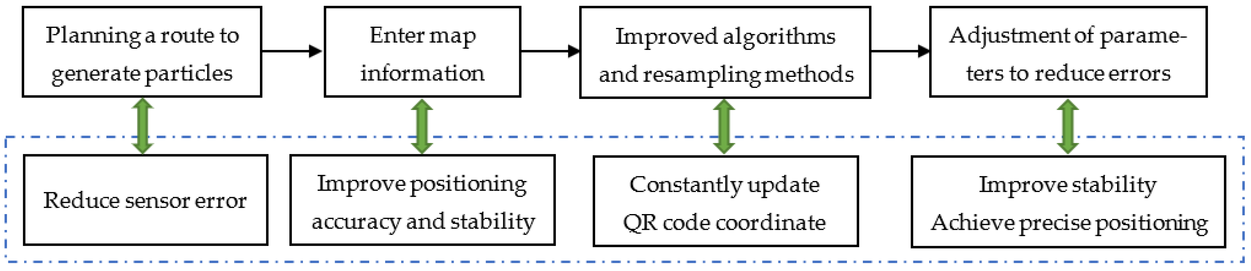
Improve the way of generating and resampling the initial particle swarm of the AMCL algorithm, so that the particle performance is more stable, and can effectively match the set template library to improve the positioning accuracy.

(2)

In the navigation process, even if the QR code is damaged and stained, it still does not affect the navigation and positioning. Hybrid navigation can complement each other and complete the navigation task independently.

(3)

The improved AMCL algorithm fuses QR code navigation. The two types of data are fused using EKF in order to improve the positioning accuracy and at the same time reduce the navigation time and improve the navigation efficiency.

(4)

The improved AMCL algorithm can effectively reduce or avoid the occurrence of particle abduction events and increase the reliability of accurate AGV positioning. The superiority of the improved algorithm can be effectively proved through field experiments.

2. Improved AMCL Algorithm

The AMCL suits local and global localization problems [21,22]. The improved AMCL algorithm can effectively solve the problem of low positioning accuracy by dynamically adjusting the number of particles and incremental particle weights and improving the resampling method, which can effectively improve the accuracy and stability of positioning.

Based on the above problem, state fusion is performed by introducing an extended Kalman filter using the outputs of the two algorithms. The different data information from the improved AMCL algorithm and the Gmapping constructed graph are fused. The map position generated using Gmapping is fused with the robot position generated by the improved AMCL, matching the AGV position estimation with the map data to obtain more accurate localization results. The improved AMCL localization algorithm inputs a parameter file to subscribe to the map information scanned using Gmapping. The sensor information received by the LiDAR is input to the AMCL positioning algorithm, and the EKF enhances the positioning accuracy by fusing the output states based on the received map data information and the AMCL positioning algorithm information. Figure 2 shows the process of data fusion between the AMCL algorithm data and lidar sweep map information by the extended Kalman filter.

2.1. AGV Motion Modelling and Chassis Structure Analysis

According to the drive mode, it is known that the AGV uses differential drive, so the motion model sketch of the QR code navigation AGV is shown in Figure 3.

As shown in the figure, the AGV dimensions $R_1$, $R_2$, and $R_3$ are: 38 cm, 30 cm, and 46 cm, respectively. The AGV is powered by a pair of differential wheels, with two followers at the front and rear supporting the AGV body. In Figure 3b, $v$ is the linear velocity of the centre of the AGV, $\omega$ is the angular velocity of the AGV, and the attitude of the AGV at the moment $t+1$ at P0. The kinematic model of the AGV is shown in Equation (1).

$$\left\{\begin{array}{c}{x}_{t+1}=x_t-\frac{v}{\omega }\sin \left({\theta }_t\right)+\frac{v}{\omega }\sin ({\theta }_t+\omega ∆t)\\ y_{t+1}=y_t-\frac{v}{\omega }\cos \left({\theta }_t\right)-\frac{v}{\omega }\cos ({\theta }_t+\omega ∆t)\\ {\theta }_{t+1}={\theta }_t+{\omega }_t\end{array}\right.$$

(1)

where $∆t$ is the sampling interval, $(x_t,y_t,z_t)$ is the attitude of the AGV at moment t, and $(x_{t+1},y_{t+1},z_{t+1})$ is the attitude at moment $t+1$.

2.2. Improving the Flow of the Algorithm

Aiming at resampling the AMCL algorithm in the iterative computation process which will increase the computation amount, an improved AMCL algorithm combining QR code information is proposed to improve the positioning accuracy, reduce the computation amount, and shorten the navigation time. The effect of the improved algorithm is shown in Figure 4.

2.3. Improved Odometer Motion Model Sampling

In the time interval $(t-1,t)$, the given motion information $u_t$ is

$$u_t=\left[\begin{array}{c}{\overline{x}}_{t-1}\\ {\overline{x}}_t\end{array}\right]$$

(2)

where ${\overline{x}}_t$ is the coordinates inside the robot; the difference between ${\overline{x}}_{t-1}$ and ${\overline{x}}_t$ enables an estimate of the difference between the two poses. The relative distances can be calculated from three steps: initial rotation ${\delta }_{rot1}$, translation ${\delta }_{trans}$, and secondary rotation ${\delta }_{rot2}$. Calculate one translation and two rotations by the given motion information $u_t$.

$$\left\{\begin{array}{c}{\delta }_{trans}=\sqrt{{\left(\overline{x}-\overline{x^{\prime }}\right)}^2+{\left(\overline{y}-\overline{y^{\prime }}\right)}^2}\hfill \\ {\delta }_{rot1}={arctan}^2\left(\overline{y^{\prime }}-\overline{y},\overline{x^{\prime }}-\overline{x}\right)-\overline{\theta }\hfill \\ {\delta }_{rot2}=\overline{{\theta }^{\prime }}-\overline{\theta }-{\delta }_{rot1} \end{array}\right.{\delta }_{trans}=\sqrt{{(\overline{x}-\overline{x^{\prime }})}^2+{(\overline{y}-\overline{y^{\prime }})}^2}$$

(3)

Since the AGV runs for a long time, it will lead to cumulative errors. The actual values of translation and rotation can be obtained by subtracting the observed value from the interference error ${\epsilon }_{b^2}$, the variance of which is $b^2$. Therefore, the motion error model can be written as:

$$\left\{\begin{array}{c}{\widehat{\delta }}_{trans}={\delta }_{trans}-{\epsilon }_{{\alpha }_1{\delta }_{trans}^2}+{\alpha }_4{\delta }_{rot1}^2+{\alpha }_4{\delta }_{rot2}^2 \hfill \\ {\widehat{\delta }}_{rot1}={\delta }_{rot1}-{\epsilon }_{{\alpha }_1{\delta }_{rot1}^2}+{\alpha }_2{\delta }_{trans}^2 \\ {\widehat{\delta }}_{rot2}={\delta }_{rot2}-{\epsilon }_{{\alpha }_1{\delta }_{rot2}^2}+{\alpha }_2{\delta }_{trans}^2 \end{array}\right.$$

(4)

${\epsilon }_{{\alpha }_1}\sim {\epsilon }_{{\alpha }_4}$ is the cumulative error of motion.

To obtain the actual location $x_t$ from $x_{t-1}$ after the initial rotation angle ${\widehat{\delta }}_{rot1}$, follow the pan delta ${\widehat{\delta }}_{trans}$, then add to another rotation angle ${\widehat{\delta }}_{rot2}$:

$$\left(\begin{array}{c}{x}^{\prime }\\ y^{\prime }\\ {\theta }^{\prime }\end{array}\right)=\left(\begin{array}{c}x\\ y\\ \theta \end{array}\right)+\left(\begin{array}{c}{\widehat{\delta }}_{trans}\cos \left(\theta +{\widehat{\delta }}_{rot1}\right)\\ {\widehat{\delta }}_{trans}\sin \left(\theta +{\widehat{\delta }}_{rot2}\right)\\ {\widehat{\delta }}_{rot1}+{\widehat{\delta }}_{rot2}\end{array}\right)$$

(5)

Then, the final odometer error is:

$$\left\{\begin{array}{c}{\delta }_{trans}-{\widehat{\delta }}_{trans}\\ {\delta }_{rot1}-{\widehat{\delta }}_{rot1}\\ {\delta }_{rot2}-{\widehat{\delta }}_{rot2}\end{array}\right.$$

(6)

2.4. Improved Resampling to Avoid Kidnapping

2.4.1. Adjustment of KLD Dynamic Resampling

The kidnapping problem refers to the fact that when the robot undergoes a drastic change in the environment or is moved to a new location, the particles in the particle filter will gather at the wrong location, resulting in inaccurate localization. In order to effectively reduce or avoid the kidnapping problem in the AMCL algorithm, this can be achieved by improving the resampling strategy of the particle filter. Traditional resampling methods, such as uniform resampling, are prone to lead to the kidnapping problem. Therefore, the kidnapping problem is avoided by using an improved KLD (Kullback–Leibler divergence resampling) sampling method to decide whether to resample or not by calculating the information entropy of the particle weights.

The Kullback–Leibler distance represents the approximation error between two probability distributions $p$ and $q$, i.e.,

$$K\left(p,q\right)=\sum _{x}p\left(x\right)log\frac{p\left(x\right)}{q\left(x\right)}$$

(7)

The Kullback–Leibler distance is non-negative and has a value of zero if and only if the two probability distributions $p$ and $q$ agree.

Assuming there is a discrete distribution with $k$ different subspaces, where the vector $X=\{X_1,X_2,X_3,\dots ,X_k\}$ represents the number of particles sampled from each subspace and the vector $P=\{P_1,P_2,P_3,\dots ,P_k\}$ represents the true probability of each subspace, the maximum likelihood estimation probability density is $\widehat{P}=\frac{X}{n}$. When n satisfies a certain number, it can be ensured that the Kullback–Leibler distance $K (\widehat{P},P)$ between the true probability density and the estimated probability density is less than a threshold value $\epsilon$, which ensures that the approximation error between the true probability density and the estimated probability density is minimized. At this point, according to the Wilson Ferty transformation method, the approximate calculation formula for n with the minimum approximation error can be obtained as follows:

$$n=\frac{k-1}{2\epsilon }{\{1-\frac{2}{9\left(k-1\right)}+\sqrt{\frac{2}{9\left(k-1\right)}}{z}_{1-\delta }\}}^3$$

(8)

where $z_{1-\delta }$ is the standard normal distribution for the upper quartile $1-\delta$.

From the above equation, the number of particles required to minimize the approximation error between the estimated and true posterior distributions can be obtained. The main purpose of particle filtering is to estimate a posterior distribution, so it is only necessary to determine the number of effective subspaces $k$ and the pre-given $\epsilon$ and $\delta$ to obtain the minimum number of particles required to ensure the estimation performance of particle filtering. It follows that the the improved KLD dynamically adjusted resampling process is as follows:

1.

Input the collection of particles $S_{t-1}=\left\{\right(x_{t-1}^{\left(i\right)},w_{t-1}^{\left(i\right)}\left)\right|i=1,\dots ,n\}$ after resampling at moment $t-1$, the observation B, set $\epsilon$ and $\delta$, the minimum value of the total number of particles $n_{xmin}$, and the number of particles $n_{t-1}$ at moment $t-1$.

2.

Set the predicted particle set at time $t$ to ${\stackrel{\sim }{s}}_t=\varnothing$, with a total number of particles of $n=1500$, a number of particles on the line $n_{xmax}=100000$, and variables $k$ and $\alpha$ both being 0. Use the dynamic adjustment method to resample particle $x_{t-1}^{\left(i\right)}$ to obtain the predicted particle $x_t^{\left(i\right)}$, and calculate the corresponding weight $w_t^{\left(i\right)}$.

3.

Accumulation of weights: ${\stackrel{\sim }{s}}_t={\stackrel{\sim }{s}}_t\cup \{x_t^{\left(n\right)},w_t^{\left(n\right)}\}$, place the newly predicted particles into the set of predicted particles $b$. If $x_t^{\left(n\right)}$ falls into the space interval $b$, then $k=k+1$, while the interval $b$ becomes non-empty.

4.

If $n\ge n_{min}$ then $n_x=\frac{k-1}{2\epsilon }{\{1-\frac{2}{9\left(k-1\right)}+\sqrt{\frac{2}{9\left(k-1\right)}}{z}_{1-\delta }\}}^3$, $n=n+1$, followed by weight orthogonalization: $w_t^{\left(i\right)}$, and finally return ${\stackrel{\sim }{s}}_t$.

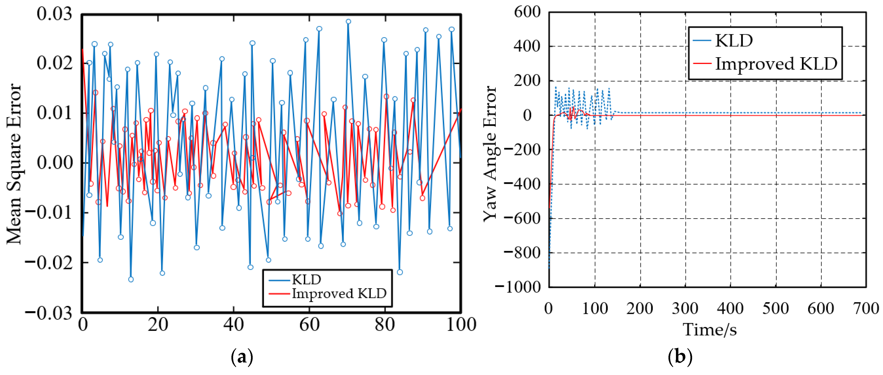
2.4.2. Simulation to Verify the Analysis of the Adjusted Dynamic Results

Verify the effectiveness of KLD dynamically adjusting resampling particles to solve the kidnapping problem through the state estimation of nonlinear systems. The simulation uses a Windows 64 bit system and the simulation software is MATLAB 2021B.

Simulation research is conducted on the state estimation problem of nonlinear systems, and the nonlinear system state equation used is as follows:

$$\left\{\begin{array}{c}{x}_k=1+\sin \left(0.04\pi k\right)+0.5x_{k-1}+v_{k-1}\hfill \\ y=\left\{\begin{array}{c}0.2x_k^2+n_k k\le 30\\ 0.5x_k-2+n_k k>30\end{array}\right.\end{array}\right.$$

(9)

where the system noise is: $v_k\sim Gamma\left(\mathrm{3,2}\right)$, and the observation noise is: $n_k\sim N\left(\mathrm{0,0.00001}\right)$.

The system noise is taken as gamma noise and the observation noise is Gaussian white noise. The initial azimuthal misalignment angle is 10°; the initial horizontal alignment angle is 1°; the accelerometer constant drift is $3\times {10}^{-5}\mathrm{g}$; the accelerometer random drift is $1\times {10}^{-5}\mathrm{g}$; the gyroscope constant drift is 0.05°/h; and the gyroscope random drift is 0.01°/h.

From the simulation results in Figure 5a, it can be seen that the KLD and the improved KLD resampling methods conclude that only the improved KLD resampling has a more stable convergence speed and consistency, and can effectively solve the fluctuation problem of particle filtering. From Figure 5b, it can be seen that the alignment accuracy and convergence speed of the improved KLD resampling are significantly better than that of the unimproved method, and the improved simulation curve eliminates the fluctuation phenomenon present in other algorithms and has better stability.

Under the same simulation conditions, the KLD and the improved KLD methods are run for 1000 steps each, and the results of calculating the mean square deviation of the state estimation of the different methods and the running time consumed by running the simulation for 1000 steps are shown in

Table 1. Comparison of alignment accuracy and runtime.

Algorithm	Standard KLD Resampling Method	Improved KLD Resampling Method
Running Time	232	75
${\varnothing }_E/(\prime )$ Variance	1.63	0.71
${\varnothing }_N/(\prime )$ Variance	1.35	0.84
${\varnothing }_U/(\prime )$ Variance	2.59	0.93

.

From Table 1, it can be concluded that the estimation accuracy of the improved KLD resampling method is better than that of the KLD method, and the computation time consumed is less than 1/2 of that of the KLD method, which evidently has a better real-time processing capability and is more suitable for real-time applications.

2.5. Improvement of AMCL Algorithm Initial Particle Swarm Generation

1.

Random sampling from Gaussian distribution to generate initial particles.

Use the global coordinate system as the reference coordinate system, use the initial positional attitude (default 0) as the mean value of the initial particle distribution, and obtain the covariance matrix of the positional attitude from the parameter server.

2.

Prediction of particle orientation.

When the odometer information is received, it is sampled from the odometer model to estimate the predicted position of the particle swarm.

3.

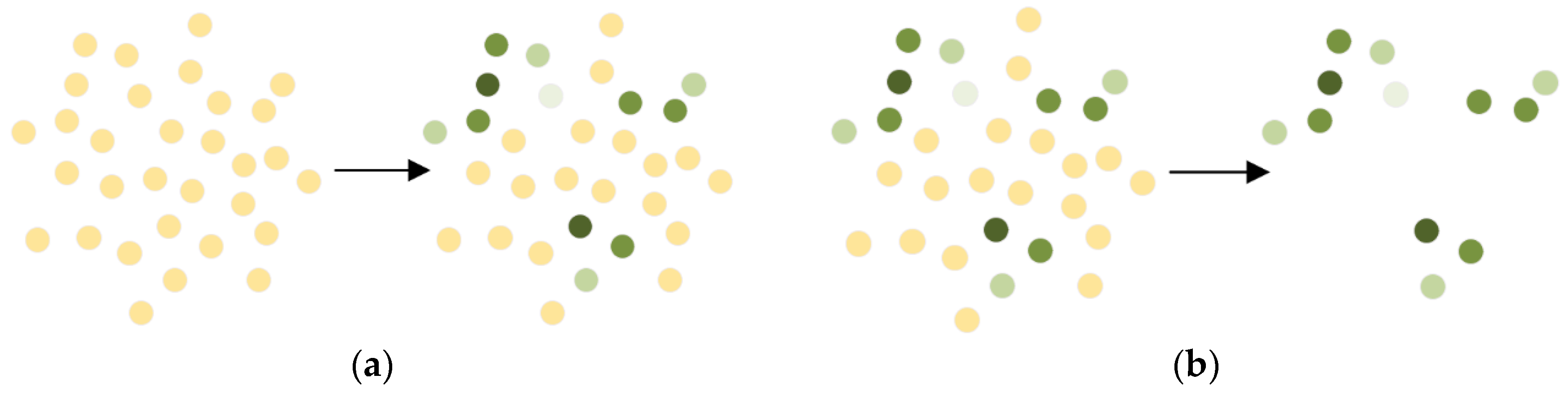
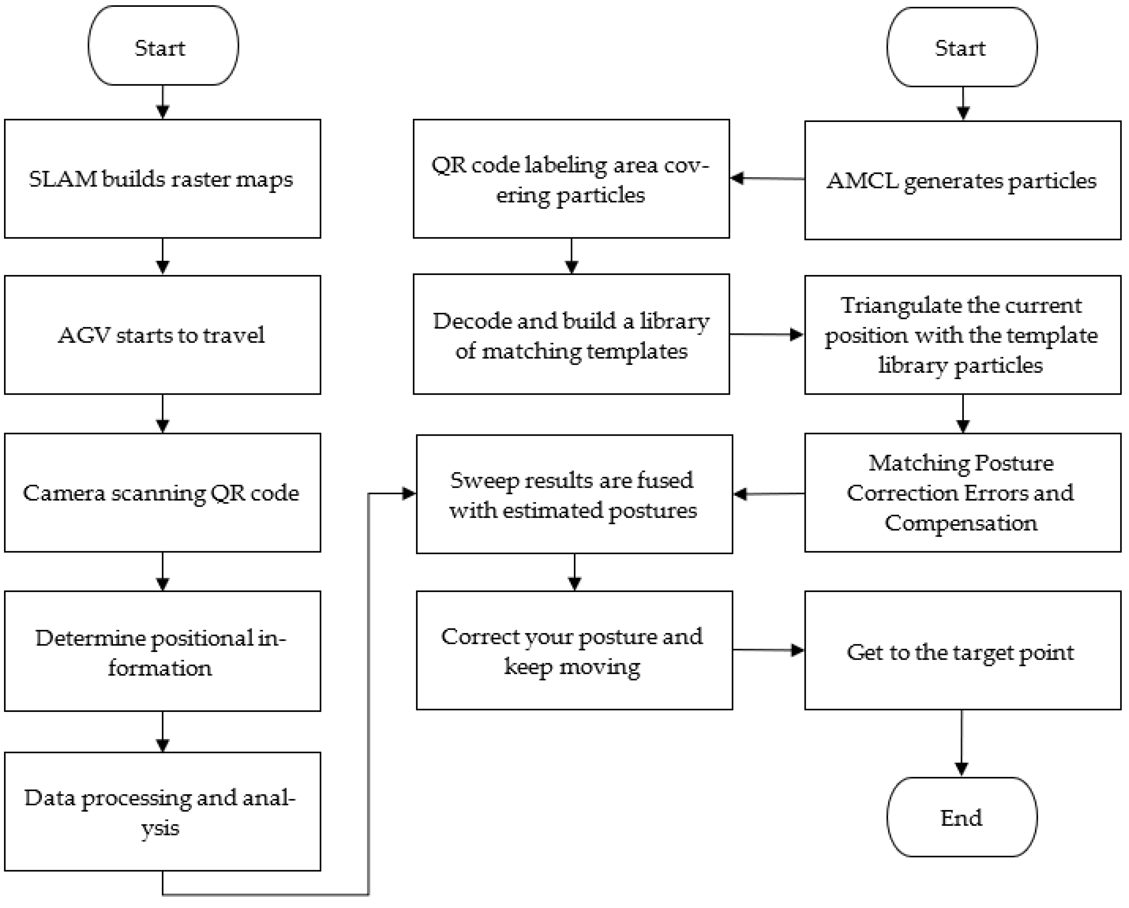
Update particle position.

When receiving the measurement data, the measurement data is put under the position of each particle, to judge the possibility of the measurement data occurring, and update the weights of the particles with this possibility. Put the laser measurement data into each particle position, and then calculate the distance between the endpoint of the laser measurement and the nearest obstacle on the map, the smaller the space is, the greater the likelihood of the laser measurement data occurring, and the greater the weight of the particle. The darker the color of the particle, the greater the weight.

4.

Resample.

If resampling, the program will judge the variance of the weights of the particle set; the larger the variance the smaller the effective particles and the more serious the particle degradation. In this case, it is necessary to carry out the resampling. After resampling, the number of particles will remain unchanged, particles with smaller weights will be filtered out, and particles with larger weights will be copied.

5.

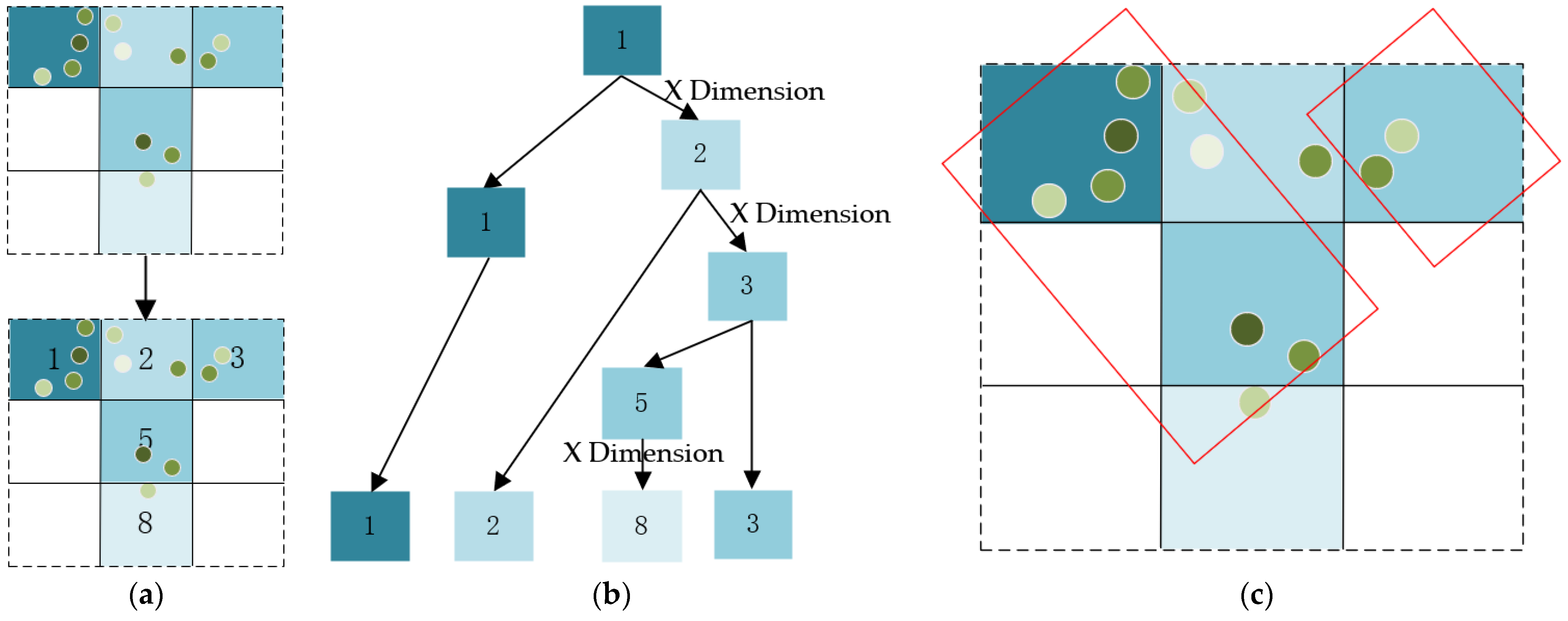
Place the resampled particles into the histogram.

The bit positions of the particles after resampling are put into the corresponding histogram. Maintain the data structure of the histogram with kd-tree, with the bit positions of the histogram as key and the weights of the particles as value. the more particles within the histogram, the darker the color of the histogram, which represents a more significant weight of that histogram.

6.

Clustering statistics results.

Recursively find if there are histograms containing particles at nine fixed distances around each histogram (here, the size of a histogram edge is used as the distance), and cluster them into one class if there are, and where it is clear that c1 is the highest-weighted class. Again, generate the variable particle swarm, find the particles in c1 and take the mean of their bit positions as the final result to publish.

Figure 6a,b represent the particle’s position information in global coordinates and the odometer’s re-prediction of the particle’s position by Gaussian noise, respectively. Figure 7a,b represent the change in the particle weights, the size of the weights based on color discrimination and the particles with larger weights are replicated, respectively. Figure 8a–c represent the process of dividing the particles based on regions, finding particles with high weights using clustering methods, and publishing particles, respectively. From the analysis of the above steps, it can be concluded that the sampling method based on the probabilistic model is used to generate the particle swarm more evenly and uniformly. According to the weights of the particles, filter out the particles with smaller weights and copy the particles with larger weights to better cover the area where the AGV is located and improve the robustness of the algorithm. For the improved initial particle swarm optimization, this can improve the initial positioning accuracy and convergence speed of the algorithm. In addition, the improved initial particle swarm generation method can also improve the accuracy of the algorithm, enabling it to effectively locate in different environments and initial conditions.

2.6. Comparison of Performance Metrics of the Improved AMCL Algorithm

The AMCL and improved AMCL algorithms are tested in simulation experiments, respectively. The simulated AGV is started on ROS with a Gmapping raster map, and the start point and end point are set to use the two algorithms for trajectory tracking planning, respectively. The distance between the cyclic Gmapping maps is 10 m, and the walking of 10 circles is one round, ten rounds. The data of each travel is recorded using a rosbag file and then imported into Matlab for simulation analysis. As shown in Figure 9, the simulation is carried out in the ROS operating system.

Where the parameters are set to $c=0 .357,\epsilon =0.2,\tau =0.05,\delta =0.01.$ The rest of the parameters were kept unchanged.

The packet rosbag obtained on ROS was imported into Matlab 2021B, after which the data was extracted to obtain the following plot of fitted and analyzed data.

The data for each of the simulations are shown in

Table 2. AMCL and improved AMCL fusion QR code algorithm comparison.

Parametric	Algorithm	Value
Maximum offset angle	AMCL	30°
	Improved AMCL	21°
Minimum offset angle	AMCL	24°
	Improved AMCL	10°
Average travel time for one lap	AMCL	7.3 s
	Improved AMCL	5.5 s
Maximum error from target point	AMCL	34 cm
	Improved AMCL	11 cm
Minimum error from target point	AMCL	24 cm
	Improved AMCL	5.2 cm

. Table 2 represents the parameter differences between the two different algorithms in the simulation case.

As can be seen from the illustration, the trace of the error is consistent with the offset error generated during AGV traveling. Still, it needs to be corrected concerning the actual speed value, a priori estimate, and a posteriori estimate. That is, the following predicted path in the process of traveling has a significant deviation from the real path, and it is easy to produce a situation in which the command route is not the same as the real route.

The improved algorithm was tested in the simulation by setting the initial yaw angle to 60°. The value change in the optimized algorithm, while ensuring that the rest of the parameters are the same, yields the silky smoothness of the real trajectory graph running over the time of (a) in Figure 10. The improved algorithm is better smoothed compared to the AMCL. (b) The grey lines in the figure serve as the measured data, with a large degree of deviation; the green lines serve as the modelled values, with a smaller degree of deviation; and the final filtered results are much closer to the true values, and the traces of error have converged to a minimum. From the figure, it can be concluded that the fluctuation is small and the performance is relatively smooth. The thin line represents the AMCL algorithm test results, and the thick line represents the improved AMCL algorithm test results. (c) and (d) in Figure 10 illustrate that the improved AMCL algorithm performs smoother for the fluctuation of the errors of the true value of the speed, the a priori estimate and the a posteriori estimate for different directions, the errors are within the permissible range, and the improvement of the algorithm meets the requirements and performs well.

3. QR Code Navigation and Construction of a Template Matching Library

The experimental simulation verifies that the improved AMCL algorithm has better performance, yielding better data in terms of positioning accuracy, arrival time and offset angle. Therefore the improved algorithm can be verified by fusion experiments.

3.1. QR Code Navigation Process

First, the AGV uses SLAM to navigate to the area near the specified QR code. Then, the AGV opens the QR code scanning function and switches to QR code navigation after scanning the QR code setting information. Then, the AGV approaches the direction of the center of the QR code until the scanning center of the AGV chassis coincides with the center of the QR code. The vehicle-mounted camera takes the position of the QR code center as the relative position, obtains the spatial coordinates through calculation and conversion, and uses the coordinate transformation to make the AGV scan the center of the QR code and realize normal movement. Figure 11 shows the flow chart of QR code scanning and recognition.

To calculate the geometric information of objects in three-dimensional space, it is necessary to calibrate the camera. From this, the camera’s internal parameter matrix A and R are obtained, and the camera’s orientation relative to the world coordinate system is determined. Since the camera’s focal length is not 0, and the matrices A and R are reversible, the actual coordinates of pixels in the photo in the AGV coordinate system are calculated using Formula (10).

$$\left\{\begin{array}{c}\left[\begin{array}{c}X\\ Y\\ Z\end{array}\right]=R^{-1}·\left(A^{-1}·{\left[\begin{array}{c}u\\ v\\ 1\end{array}\right]}^{-1}\right)\\ \left(u_c,v_c\right)=\left(\frac{u_1+u_3}{2},\frac{v_1+v_3}{2}\right)\hfill \end{array}\right.$$

(10)

When the central coordinate of the QR code $p(u_c,v_c)$ is known, the coordinates $\mathsf{{\rm P}}({\mathrm{X}}_C,{\mathrm{Y}}_C,{\mathrm{Z}}_C)$ of the car body coordinate system can be calculated. Due to the use of QR code three-point positioning, the coordinates of the three points of the QR code in the image $(u_1,v_1)$, $(u_2,v_2)$, $(u_3,v_3)$, and because the position of the required detection pattern is known, the coordinates of the center $p(u_c,v_c)$ of the QR code can be calculated, and $p(u_c,v_c)$ is substituted to obtain the coordinates $\mathsf{{\rm P}}({\mathrm{X}}_C,{\mathrm{Y}}_C,{\mathrm{Z}}_C)$ of the QR code in the coordinate system of the car body. Combined with the coordinate information of the current QR code in the entire map, the position of the AGV in the map can be determined. In Figure 12 (a) represents the relationship between the three coordinate systems, (b) AGV scanning for coordinate transformation.

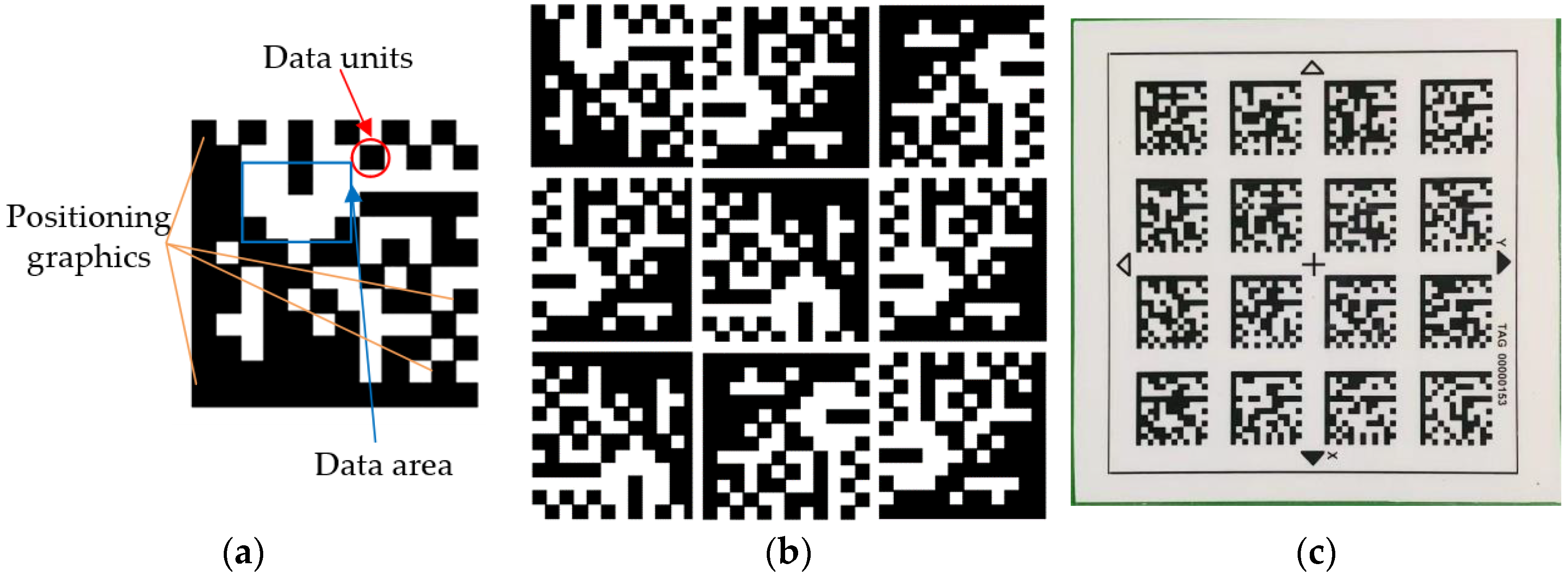
3.2. Construction of the Template Matching Library

The stability of QR code navigation depends on the performance of the reader (decoding speed, accuracy, and precision) and the performance of the IMU (accuracy and stability) [23,24]. The higher the decoding efficiency of the reader, the higher the AGV can travel. However, if the QR code is dirty and damaged, the navigation accuracy will significantly decrease. Therefore, we propose a library of QR code templates to improve the positioning accuracy. QR codes of the same size with different recognition areas are generated by a QR code generator, and each QR code template library contains nine independent QR codes, each of which is unique. In other words, multiple QR codes are fused into a QR code combination map, and the QR code template libraries are constructed based on the “different codes” in the QR code recognition area, and the current pose is quickly determined by triangulation matching.

To further improve the localization accuracy of QR code labels in the global graph, a particle-based localization algorithm in AMCL is used to match the QR code combination graph. The Gmapping grid map is drawn using SLAM navigation. Use the three points of the QR code identification area to form a triangle as the coordinate position of the QR code (the QR code itself also stores the position information), and save it in the map. The location of the QR code label is used as a landmark, and the AGV recognizes its ID by matching the triangles and obtains the corresponding coordinates when it detects the QR code landmark. Since each QR code tag area generates different particles, but the template library is unique, the similar triangles identified above for triangle matching can be matched with the template library. As shown in Figure 13a shows the graphic and storage information area of the QR code, Figure 13b shows the formation of QR code landmarks through multiple QR codes, and Figure 13c shows the QR code landmarks affixed to the experimental site. For example, when different numbers of particles are generated at the position of the label of the template library in the front A, then scanning the position in front can obtain a lot of similar triangles according to the different positions of the particles, at this time, the triangles generated by the particles in the fixed area are matched with the triangles of the current correct position area, which is similar but the direction is different, and thus the AGV is automatically adjusted to the angle. Therefore, the distance and offset angle between the AGV and the label can be determined. Firstly, the AGV calculates the relative position of the QR code tag in the SLAM global map based on the received QR code data, thus obtaining the approximate orientation of the detected QR code. Then, the AGV performs a self-tracking motion based on the approximate position in the map and quickly determines the part of the QR code label based on triangle matching.

The matching template library formula is as follows:

$$\begin{array}{c}{l}_{49},l_{48},l_{89},(x_4,y_4),(x_8,y_8),(x_9,y_9),1\\ l_{48},l_{18},l_{14},(x_1,y_1),(x_4,y_4),(x_8,y_8),2\\ l_{33},l_{12},l_{26},(x_3,y_3),(x_7,y_7),(x_5,y_5),3\\ ⋮\\ l_{xy},l_{xy},l_{xy},(x_x,y_y),(x_x,y_y),(x_x,y_y),r\\ ⋮\\ l_{xy},l_{xy},l_{xy},(x_x,y_y),(x_x,y_y),(x_x,y_y),n\end{array}$$

(11)

In the above equation, $l_{xy}$ is the edge length of the triangle template library, and $(x_x ,y_y)$ is the coordinate value of each point.

In this paper, we use the estimated position of the AGV as the input to fuse the world coordinates of the QR code and increase the weight of particles in the AMCL algorithm. Many QR code landmarks were detected in the process of AGV moving, and the location of QR code landmarks was quickly determined according to the triangle matching. The relationship between the AGV and the detected QR code landmark is as follows:

$$\begin{array}{c}{\left(x_V-x_1\right)}^2+{\left(y_V-y_1\right)}^2=r_1^2\\ {\left(x_V-x_2\right)}^2+{\left(y_V-y_2\right)}^2=r_2^2\\ ⋮\\ {\left(x_V-x_i\right)}^2+{\left(y_V-y_i\right)}^2=r_i^2\\ ⋮\\ {\left(x_V-x_n\right)}^2+{\left(y_V-y_n\right)}^2=r_n^2\end{array}$$

(12)

where $(x_V,y_V)$ represents the estimated position of the AGV car, which can be obtained by solving the formula. $(x_i,y_i)$ is the $i$th location of the QR code detected. In addition, it can be obtained that the direction of the AGV is

$${\theta }_V=\left\{\begin{array}{c}\begin{array}{c}\frac{1}{n}{\displaystyle \sum _{i=1}^n}\left[\arctan \left(\frac{y_i-y_V}{x_i-x_V}\right)-{\phi }_i\right] x_i>x_V \hfill \\ \frac{1}{n}{\displaystyle \sum _{i=1}^n}\left[\arctan \left(\frac{y_i-y_V}{x_i-x_V}\right)-{\phi }_i+\pi \right] y_i\ge y_V, x_i<x_V\hfill \\ \frac{1}{n}{\displaystyle \sum _{i=1}^n}\left[\arctan \left(\frac{y_i-y_V}{x_i-x_V}\right)-{\phi }_i-\pi \right] y_i<y_V, x_i<x_V \hfill \end{array}\hfill \\ \frac{1}{n}{\displaystyle \sum _{i=1}^n}\left[\frac{\pi }{2}-{\phi }_i\right]{ y}_i>y_V, x_i=x_V\hfill \\ \frac{1}{n}{\displaystyle \sum _{i=1}^n}\left[-\frac{\pi }{2}-{\phi }_i\right] { y}_i<y_V, x_i=x_V\hfill \end{array}\right.$$

(13)

where ${\theta }_V$ represents the direction of the AGV car and $\phi$ is the observation angle of the detected QR code landmark. Therefore, the estimated pose of the AGV car can be expressed as ${\mu }_V=(x_V,y_V,z_V)$.

The estimated position of the AGV car can be obtained from Equations (12) and (13), and the position weight of the particle can be calculated as follows:

$$d^{\left[i\right]}={\frac{1}{{(2\pi )}^{\frac{3}{2}}}\mathsf{{\rm E}}\mathsf{{\rm X}}\mathsf{{\rm P}}(-\frac{1}{2}(x_t^{\left[i\right]}-{\mu }_V)}^{\mathsf{{\rm T}}}(x_t^{\left[i\right]}-{\mu }_V))$$

(14)

where the position and direction of the particle are $x_t^{\left[i\right]}=(x_i,y_i,{\phi }_i)$.

The AMCL algorithm covers the whole map evenly, and then the particles converge near the QR code according to the location of the QR code landmark. As shown in Figure 14a,b. When scanning the QR code landmark at a specific location, triangular matching joins to the QR code landmark. As in Figure 14c. The coordinates of $a$, $b$, and $c$ are $(x_a,y_a)$, $(x_b,y_b)$, and $(x_c,y_c)$, respectively. The side lengths of the three measured triangles are $l_{ab}$, $l_{ac}$, and $l_{bc}$, respectively. First, search for similar triangles in the QR code template library. As in Figure 14d. The three sides are unequal in length but proportional, and the angles are equal. Thus, the detected $∆abc$ matches the $∆$835 in the library. As in Figure 14e,f.

Triangle detected:

$$l_{ab},l_{ac},l_{bc},\left(x_a{y}_a\right),\left(x_b{y}_b\right),\left(x_c{y}_c\right)$$

(15)

Matching template library:

$$\left\{\begin{array}{c}{l}_{49},l_{48},l_{89},\left(x_8,y_8\right),\left(x_3,y_3\right),\left(x_5,y_5\right),1\\ ⋮\\ l_{28},l_{29},l_{89},\left(x_2,y_2\right),\left(x_8,y_8\right),\left(x_9,y_9\right),k\\ ⋮\\ l_{35},l_{34},l_{55},\left(x_1,y_1\right),\left(x_3,y_3\right),\left(x_9,y_9\right),n\end{array}\right.$$

(16)

Triangular matching identification:

$$\left\{\begin{array}{c}a\left(x_a,y_a\right)=8\left(x_8,y_8\right)\\ b\left(x_b,y_b\right)=3\left(x_3,y_3\right)\\ c\left(x_c,y_c\right)=5\left(x_5,y_5\right)\end{array}\right.$$

(17)

In the navigation process, the completeness and accuracy of the constructed map is one of the decisive factors in determining the accuracy of navigation and positioning [25]. Significant errors in map construction often directly lead to problems such as positioning failure and unguaranteed accuracy [26]. To improve the map-matching accuracy in navigation, the weight of the particles in the AMCL algorithm is increased in the code reading area. Then, the AGV position information is updated, and the data is estimated to be within the normal range according to the recognition of the new.

Establish a simulation environment and analyze and improve the various types of problems that occur in the algorithm through simulation experiments to verify the algorithm. Figure 15 and Figure 16 represent the fusion process of QR codes in the simulated state and in the improved algorithmic positioning shown simultaneously in the RVIZ and Gazebo environments, respectively.

3.3. Extended Kalman Filter Fusion Data

The estimated position of the QR code navigation AGV sweep data and the AMCL algorithm can be fused by a fusion method to obtain a more accurate position estimation [27,28]. In the fusion process, it is first necessary to convert the QR code navigation AGV scanning data into positional information, which is usually obtained by decoding the QR code to obtain the position and attitude information of the QR code. Then, this position information is fused with the estimated position of the AMCL algorithm. The fusion method is as follows:

1.

Prediction steps.

Establishing the equation of state:

$$X_{k+1}=\left[\begin{array}{c}{x}_k\\ y_k\\ v_k\\ {\theta }_k\\ {\omega }_k\end{array}\right]+\left[\begin{array}{c}{v}_k·\cos \left(\theta \right)·∆t\\ v_k·\sin \left(\theta \right)·∆t\\ 0\\ \omega ·∆t\\ 0\end{array}\right]+\left[\begin{array}{c}\frac{1}{2}·{\alpha }_{v,k}·\cos \left(\theta \right)·∆t^2\\ \frac{1}{2}·{\alpha }_{v,k}·\sin \left(\theta \right)·∆t^2\\ {\alpha }_{v,k}·∆t\\ \frac{1}{2}·{\alpha }_{\omega ,k}·∆t^2\\ {\alpha }_{\omega ,k}·∆t^2\end{array}\right] , {\omega }_k\ne 0$$

(18)

where $x$ is the $x$-direction coordinate, $y$ is the $y$-direction coordinate, $v$ is the radial velocity, $\theta$ is the yaw angle, $\omega$ is the yaw angular velocity, ${\alpha }_{v,k}$ is the acceleration of the radial velocity $v$, and ${\alpha }_{\omega ,k}$ is the acceleration of the yaw angular velocity $\omega$.

Condition prediction:

$${\widehat{x}}_{k+1|k}=\left[f({\widehat{x}}_{k|k}\right)+F_k\left(x_k-{\widehat{x}}_{k|k}\right)+{\omega }_k]$$

(19)

where $f\left({\widehat{x}}_{k|k}\right)$ is the state estimate, $x_k$ is the state vector, and $F_k$ is the higher order term derivation.

From Equations (18) and (19) the predicted covariance prediction can be derived as

$$P_{k+1|k}={[F}_k\left(x_k-{\widehat{x}}_{k|k}·\cos \left(\theta \right)∆t\right)+{\alpha }_{v,k}·∆t]·{[F}_k\left(x_k+{\widehat{x}}_{k|k}·\sin \left(\theta \right)∆t\right)-{\alpha }_{\omega ,k}·∆t^2]$$

(20)

2.

Update steps.

Convert the QR code navigation AGV scanning data into an observation model, i.e., the position and attitude information of the QR code is converted into a positional observation. Compare the observation model with the predicted position and attitude, and calculate the observation residuals:

$$\widehat{y}=z_k-H_k{\widehat{x}}_{k|k+1}$$

(21)

$z_k$ is the state estimation transfer equation and $H_k$ is the observation matrix.

$$\left\{\begin{array}{c}{z}_k=H_k·x_k+v_k\\ x_k=F_k{x}_{k-1}+B_k{u}_k+{\omega }_k\end{array}\right.$$

(22)

$v_k$ is the observation noise and $B_k$ is the input control model acting on the controller vector $u_k$.

Calculate the Kalman gain:

$$K_k={\widehat{P}}_k·H^T·{(H·{\widehat{P}}_k{H}^T+R)}^{-1}$$

(23)

$R$ is the measurement noise covariance matrix and $H$ is the measurement matrix.

Based on the Kalman gain and observation residuals, the updated bit position estimate is

$$h\left(x^{\prime }\right)=\left[\begin{array}{c}\rho \\ \psi \\ \dot{\rho }\end{array}\right]=\left[\begin{array}{c}\sqrt{P_x^2+P_y^2}\\ \arctan \left(\frac{P_x}{P_y}\right)\\ \frac{P_x{V}_x+P_y{V}_y}{\sqrt{P_x^2+P_y^2}}\end{array}\right]$$

(24)

where $P_x$, $P_y$, $V_x$, and $V_y$ are the positions and velocities of the fused a priori estimates.

3.

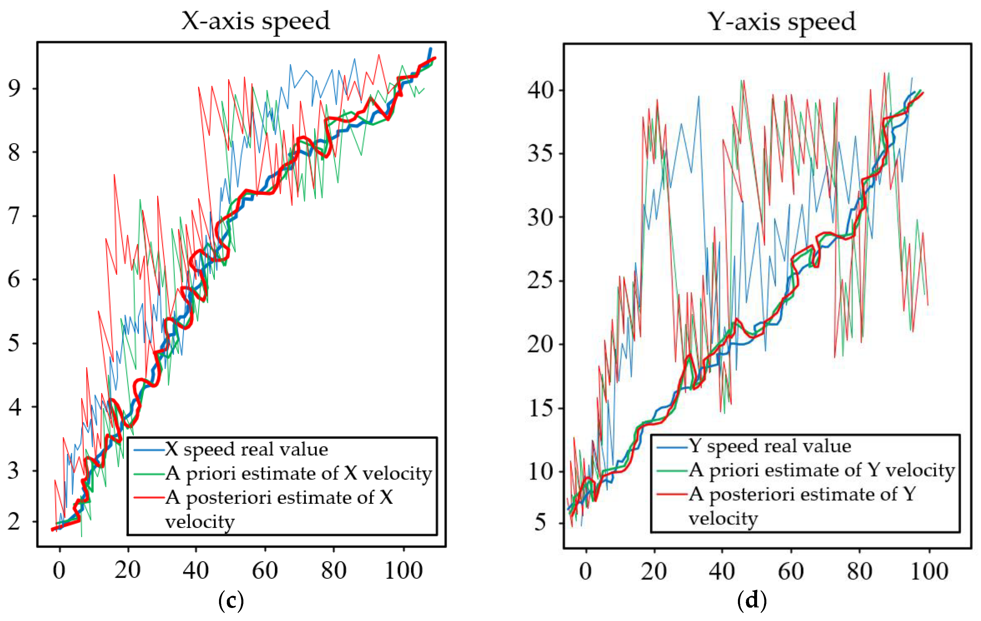
Simulation result diagram.

The two were fused for simulation to test the correlation relationship.

Figure 17 shows the accuracy test of the EKF fusion data. Simulations using EKF fused data can yield close to the true values and can be used with this fusion method.

4. Experimental Validation

In order to verify the effectiveness of the proposed combination algorithm, a simulation platform is established and real experimental scenarios are built to verify the effectiveness. The AGV used in the simulation is 0.5 m × 0.3 m × 0.2 m in size, with a mass of 10 Kg, LIDAR on top, and an inertia matrix of ${[0.01, 0, 0; 0, 0.02, 0; 0, 0, 0.03]}^T$. The mean value of the measurement noise is set at 0, and the covariance matrix at $[0.01, 0; 0, 0.01]$, which means that the variance of the measurement noise in the x- and y-directions is 0.01.

The parameters are set for simulation experiments and the rest of the data is kept constant. The data obtained in the simulation experiment platform is analyzed using MATLAB2021B.

Table 3. AGV setup parameters.

Name	Number
Maximum linear speed	$1 \mathrm{m}/\mathrm{s}$
Maximum angular velocity	$1 \mathrm{rad}/\mathrm{s}$
Maximum linear acceleration	$0.5 \mathrm{m}/{\mathrm{s}}^2$
Maximum angular acceleration	$0.5 \mathrm{rad}/{\mathrm{s}}^2$
Radar scanning angle	$320°$
Radar scanning frequency	$10 \mathrm{Hz}$
Maximum measurement distance of radar	$10 \mathrm{m}$
Improved AMCL algorithm particle initial value	$1000$
Resampling measurement	Low variance resampling

shows the parameter settings of the AGV.

4.1. Improved AMCL Algorithm Simulation Comparison Experiment

A raster map is generated using SLAM laser navigation, and AMCL localization particles are tiled over the raster map until the whole map is tiled. The AMCL algorithm and the improved AMCL algorithm are introduced separately, and the different situations among the two are observed and data is collected for analysis. The size of the map is 10 m × 10 m, and travelling one lap is recorded as one complete distance.

Navigation was tested using different algorithms in the same environment, and Figure 18 show the different scenarios in which the particles behaved separately.

Photoelectric sensors were set up on both sides of the laying of the QR code and at the start-end position to detect the number of corrections and the maximum distance of error when different algorithms were used for tracking the trajectory, in order to record a week’s navigation time as well as the maximum distance from the set point of the target error.

It can be learnt from the distribution of the particles that the distribution of the improved algorithm particles performs better compared to the previous algorithm, distributing on the real trajectory with less error, and the rest of the particles of the regions not involved by the AGVs disappear, only in the aggregation of the labels. From Figure 19 it can be seen that during approximately the first 30 messages released by the AMCL, the localization error is small; once 30 messages are released, the AGV is abducted to produce a large error. As the AGV moves, the positioning error gradually decreases, and after multiple messages, the error tends to 0, restoring the original positioning accuracy. Although the improved AMCL algorithm also encounters kidnapping, the adjustment time is improved by 68.73% compared to the unimproved algorithm.

The maximum data for the offset recorded by the photoelectric sensor in Figure 20a is (−18.79, 22.38) when using the AMCL algorithm, while the improved AMCL algorithm is (−4.79, 6.82). That is to say, adjusting the trajectory to the left exceeds the set trajectory line by a maximum of 22.83 cm and 6.82 cm, and adjusting the trajectory to the right exceeds the distance by a maximum of 18.79 cm and 4.79 cm, from which the comparison can be significantly concluded that the improved algorithm is superior. Figure 20b with the increase in the running time, the error gradually increases and reaches a peak at a certain point, and then the error gradually decreases, but the adjustment time also gradually increases. In contrast, because of the addition of the algorithm to eliminate the cumulative error link, in the improved algorithm, the error will be adjusted quickly with a slight difference between the scan data and the simulation algorithm. Because of the large deviation, the velocity variation is large, the maximum velocity cannot be reached, and the velocity variation has to be adjusted in each sweep, and the fluctuation of linear and angular velocities in Figure 20c,d are fluctuate more compared to the improved AMCL algorithm.

Table 4. AMCL and improved AMCL fusion QR code algorithm comparison.

Parametric	Algorithm	Value
Starting particle	AMCL	1500
	Improved AMCL	1500
Time from start to target (10-turn average)	AMCL	12.59 s
	Improved AMCL	7.42 s
Offset maximum distance (both sides)	AMCL	(−18.79, 22.38) cm
	Improved AMCL	(−4.79, 6.82) cm
Deviation distance to target point (10-turn average)	AMCL	27.36 cm
	Improved AMCL	4.81 cm
Dissolution of kidnapping recovery time (10-turn average)	AMCL	2.2 s
	Improved AMCL	0.39 s

shows the performance of different algorithms with the same conditions.

4.2. Real Scene Experimental Test

The simulation experiments have proved that the proposed algorithm has good performance and the localization time and error distance are greatly reduced, so it can be significantly shown that the improved AMCL algorithm has better superiority. Therefore, the real effectiveness of the improved algorithm is verified, and the experiments are carried out and analyzed in real scenarios. Figure 21a,b shows the front and side view of the AGV used in the experiment. Figure 21c shows the experimental site used in the experiment, and Figure 21d shows the QR code labels pasted in the experimental site.

Real experimental scenarios are established and tested using the improved AMCL algorithm to obtain valid data for analyzing the reliability of the algorithm.

The map generated using the SLAM technique is shown in Figure 22, where the thin green line from 0 to 1 is the trajectory of the AGV. The round-trip is one lap, and the data of the AGV travelling ten laps are saved and imported into MATLAB2021B for analysis, which proves the validity of the proposed algorithm by comparing the data with the positional error of AGV arriving at the target point, the maximal corrective angle, the speed fluctuation, and line acceleration.

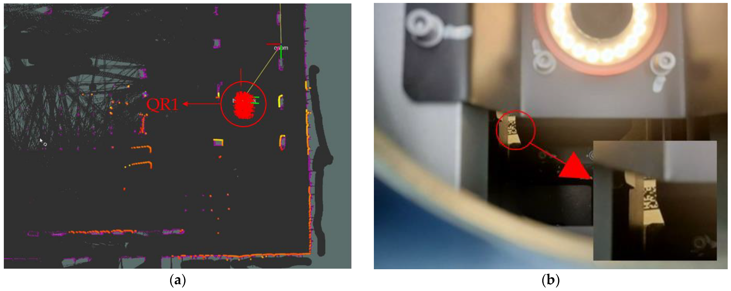
4.2.1. Improved AMCL Matching Template Library Accuracy Test

Use SLAM to generate particles on the QR code, mark the coordinate position of the QR code on the map, turn off the camera, use the particles to determine the coordinate position of the QR code, and the AGV travels to the particle aggregation area until it reaches the matching QR code marking point. Compare the position information with the actual coordinate position information of the QR code and analyze the error distance between the two.

Figure 23a shows that the improved AMCL particles converge on the QR1 position, at which time, Figure 23b shows that the AGV stopping position is in the area directly above the landmark. From the actual test, it is concluded that the AGV identifies the particle template on QR1 to match the exact position of the first landmark on the SLAM construction map, and then accurately travels to the first landmark area location, waiting for the next command. At this time, the industrial camera is opened to scan the code, and the real position of the AGV at this time is obtained through coordinate conversion, comparing the coordinate information and measuring the position error interval between the particle triangular matching position information using the improved AMCL algorithm and the position error interval of the QR code scanning information.

Taking the forward direction of the AGV as the y-axis and the left-right offset distance as the x-axis, two photoelectric sensors are installed before and after the QR1 landmark position, and the coordinate information of each arrival position is re-recorded and weighted average.

Table 5. AMCL and improved AMCL fusion QR code algorithm comparison.

Average Value	Actual Position Coordinates	Particle Triangulation Matching Position Coordinates	Industrial Camera Scanning Position Coordinates	Scanning Fusion Improved AMCL	Maximum Left Offset Maximum Right Offset
Cycle 5 times	(0, 375.00) cm	(1.96, 377.92) cm	(3.24, 373.16) cm	(0.59, 374.25) cm	(0.88, 0.53) cm
Cycle 10 times	(0, 375.00) cm	(2.88, 373.40) cm	(2.64, 377.88) cm	(0.36, 375.40) cm	(0.56, 0.62) cm
Cycle 20 times	(0, 375.00) cm	(3.72, 377.34) cm	(1.52, 377.50) cm	(0.42, 375.34) cm	(0.78, 0.62) cm
Cycle 30 times	(0, 375.00) cm	(2.48, 373.68) cm	(2.44, 373.32) cm	(0.44, 375.32) cm	(0.84, 0.66) cm
Cycle 50 times	(0, 375.00) cm	(1.54, 377.12) cm	(3.72, 377.48) cm	(0.72, 374.48) cm	(0.76, 0.64) cm

shows that the combination of code-sweeping positioning and improved AMCL algorithm has the highest accuracy, with the maximum offset of coordinate information not exceeding 1 cm, and the reading distance before and after the combination not exceeding 0.5 cm, and the navigation and positioning accuracy has been improved by 64.27% on the original basis.

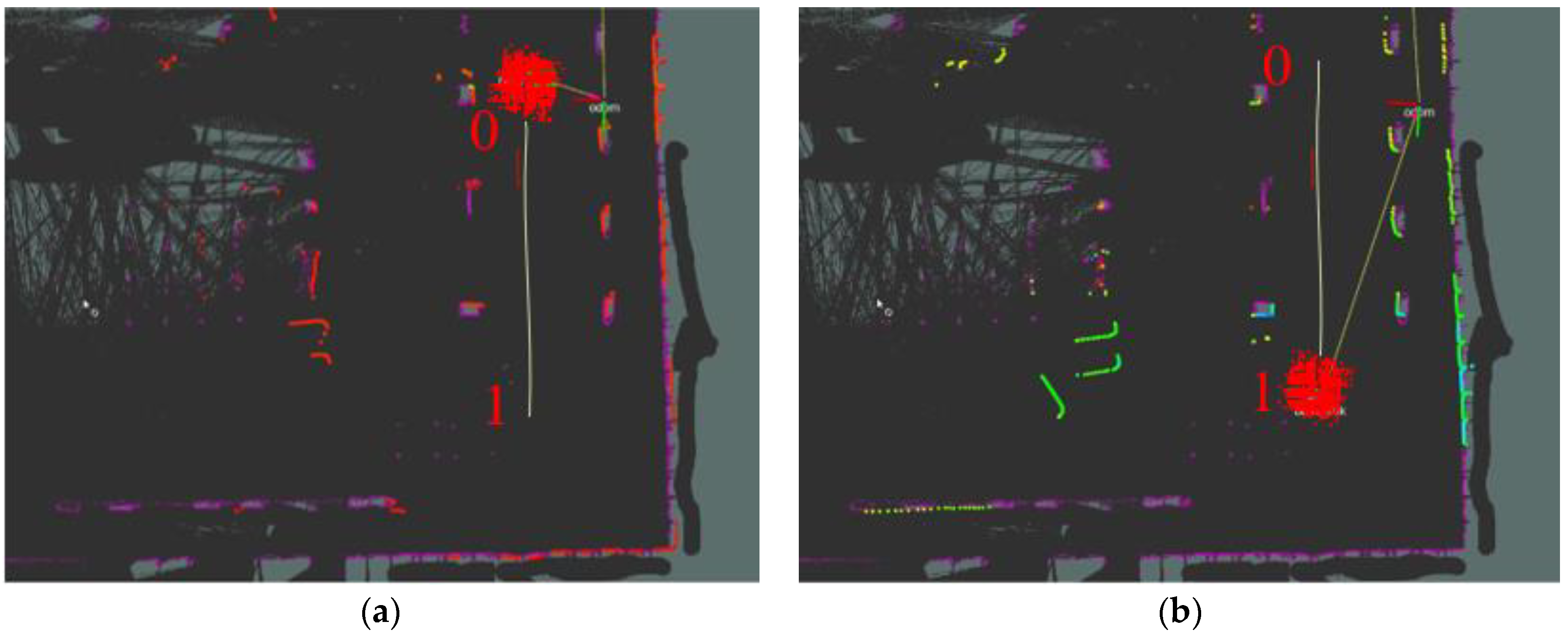
4.2.2. AGV Particle Kidnapping Experiment

In previous simulation experiments, it was found that the particles generated by the AMCL algorithm were prone to kidnapping events during the positioning process. The improvement of the algorithm as well as the improvement of resampling can effectively avoid such situations, so it is verified in real experiments that the algorithm can effectively improve the robustness and reliability of AGV positioning.

The experiments show that the particles in the AMCL algorithm will not disperse automatically after AGV is kidnapped, so it is impossible to relocate. However, the improved AMCL algorithm will scatter some particles at the kidnapped position, which can be relocated. Figure 24 shows the process of the kidnapping and location recovery of the AGV when the improved AMCL algorithm is started. Figure 24a shows the initial state of the AGV. At this time, the AGV is ready to accept the command to move forward, and the particles are in a dispersed state. Figure 24b shows the state that the AGV moves to QR2 point, at which time the particles are in a convergent state. Figure 24c shows that the AGV is kidnapped, and the particles gather in this area and do not diverge with the movement of AGV. As shown in Figure 24d, to detect the kidnapping event, the improved algorithm is adjusted and the positioning state is restored. To calculate the kidnapping time, calculate the duration of the kidnapping time based on the start time and end time of the kidnapping event. To monitor the positioning error, sensors or other positioning systems are used to monitor the difference between the actual position of the AGV and the position estimated by the AMCL algorithm. When the positioning error exceeds a certain threshold, it can be determined that an kidnapping event has occurred. Record the start time of the abduction event. When the positioning error exceeds the threshold, record the current time as the start time of the kidnapping event. To monitor the positioning recovery, continue to monitor the positioning error, and when the positioning error recovers to within an acceptable range, it can be judged that the kidnapping event is over.

The AGV was driven for 10, 20, and up to 50 laps, respectively, for the experimental testing, the time used when the kidnapping event occurred and the time after adjustment were recorded, and the data were analysed and counted in

Table 6. Measurements of the occurrence of kidnappings.

Number of Cycles	Algorithm	Number of Kidnapping Incidents	Cumulative Time /Average Time (s)	Maximum/Minimum Recovery Time (s)	Maximum/Minimum Positioning Error (cm)
10	AMCL	17	51.64/3.04	2.59/1.75	22.81/15.69
	Improved AMCL	2	1.18/0.59	0.12/0.06	3.88/1.72
20	AMCL	31	79.04/2.54	2.78/1.16	19.26/10.71
	Improved AMCL	3	1.56/0.52	0.21/0.02	4.33/2.28
30	AMCL	44	119.68/2.72	2.13/1.54	21.16/9.31
	Improved AMCL	5	2.26/0.45	0.51/0.03	3.29/1.61
40	AMCL	60	146.28/2.44	2.88/1.02	18.74/11.26
	Improved AMCL	8	3.28/0.40	0.96/0.02	5.10/2.13
50	AMCL	71	162.64/2.29	1.35/0.97	16.89/8.92
	Improved AMCL	10	4.18/0.41	0.29/0.05	3.77/1.02

. From Table 6, it can be clearly concluded that the use of the improved AMCL algorithm can effectively avoid the occurrence of kidnapping events, and the solution of the kidnapping problem can save 42.81% of the AGV navigation time, and once such an event occurs, it can be quickly adjusted to avoid the problem of inaccurate positioning in the process of moving forward.

4.3. Discussion

QR code-navigated AGVs are widely used in agriculture, industrial automation, healthcare, logistics, and other fields. There are a large number of researchers contributing to QR code navigation, localization, path planning, etc. in the related literature. With the development of industrial automation, visual navigation is widely adopted because of its high accuracy and low latency. However, single navigation still faces many problems, such as a long processing time and high sensor requirements. Ref. [7] proposed to use EKF combined with an internal encoder and external QR code to correct the cumulative error generated by attitude estimation. This method can effectively solve the error problem and improve the positioning accuracy, providing a new reference for navigation methods. However, the error increases as the distance of the QR code paste increases.

In this article, EKF can only calculate the a posteriori estimate of the state through the current measurement value and the a priori estimate, and cannot directly consider the influence of historical data, so it is susceptible to the cumulative error of the sensor. EKF assumes that the noises in the system model and the measurement model are linear Gaussian distributed, but there may be nonlinear noises and non-Gaussian distributed noises in the actual application, which may lead to the filtering results of accuracy degradation. Our work meets the positioning requirements of high-precision navigation systems in terms of adaptive tuning, positioning accuracy, and navigation time.

When in a suitable environment, the navigation and positioning scheme proposed by some researchers can achieve 100% positioning and permanently eliminate accumulated errors. The method proposed by [8] can achieve 100% accuracy and complete given commands under suitable circumstances. It has achieved a qualitative leap in the field of navigation and positioning. However, due to its use of RGB sweep detection, when encountering bright light environments, or when obstacles are similar in color to the transported object, it can adversely affect the results to detect the completion of instructions.

Zhang, H., and Dong, S. et al. [29,30] proposed different fusion methods to improve the positioning accuracy and reduce the time required for navigation. However, when AGVs are in an environment similar to a long corridor, they are prone to map distortion, incorrect judgement of current position, continuing along the wrong route and collision problems.

Through the simulation experiments and scenario tests in this section, a large number of experimental comparisons can be made to conclude the superiority of the proposed method in this paper, which is better than similar methods in terms of the adaptive adjustment time, positioning accuracy, and navigation time.

5. Conclusions

This paper introduces an AGV navigation and positioning system that integrates navigation and precise positioning. The AMCL particle positioning algorithm is used to perform triangular matching, establish a library of QR code templates, and quickly identify the current position of the QR code for precise positioning. The accuracy of the proposed algorithm is verified through a large number of comparative experiments and simulation data, and the positioning and navigation tasks can be completed in a real experimental environment. It solves the problems of inaccurate positioning and low precision, which are common in the market at present, and provides reference for the accurate positioning of AGV. The focus of this research is to develop hybrid navigation AGVs based on the market scarcity to serve the public and shift from industry to service. The main contributions of this paper are as follows:

1

This article provides an in-depth analysis and research on the development status of AGV’s critical domestic and international technologies and researches robot navigation, positioning, and path planning technology. The advantages and disadvantages of various methods are compared, and the overall navigation scheme and system navigation method are designed in detail. Finally, the feasibility and benefits of this choice are verified through experiments.

2

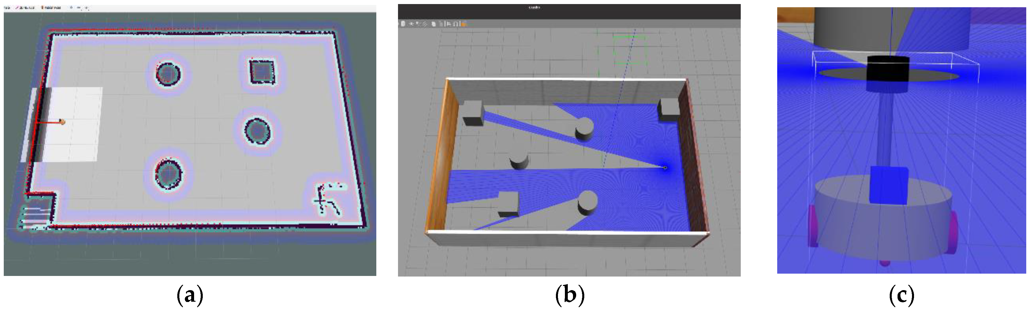
An ROS operating system was used to build the simulation environment of the AGV, and the real positioning system platform was established to prepare for the research of the AGV positioning system. The localization system proposed in this paper uses SLAM global mapping to obtain the absolute coordinates of ground punctuation. It uses the improved AMCL algorithm to combine QR codes, which improves the positioning time and accuracy in the navigation process.

3

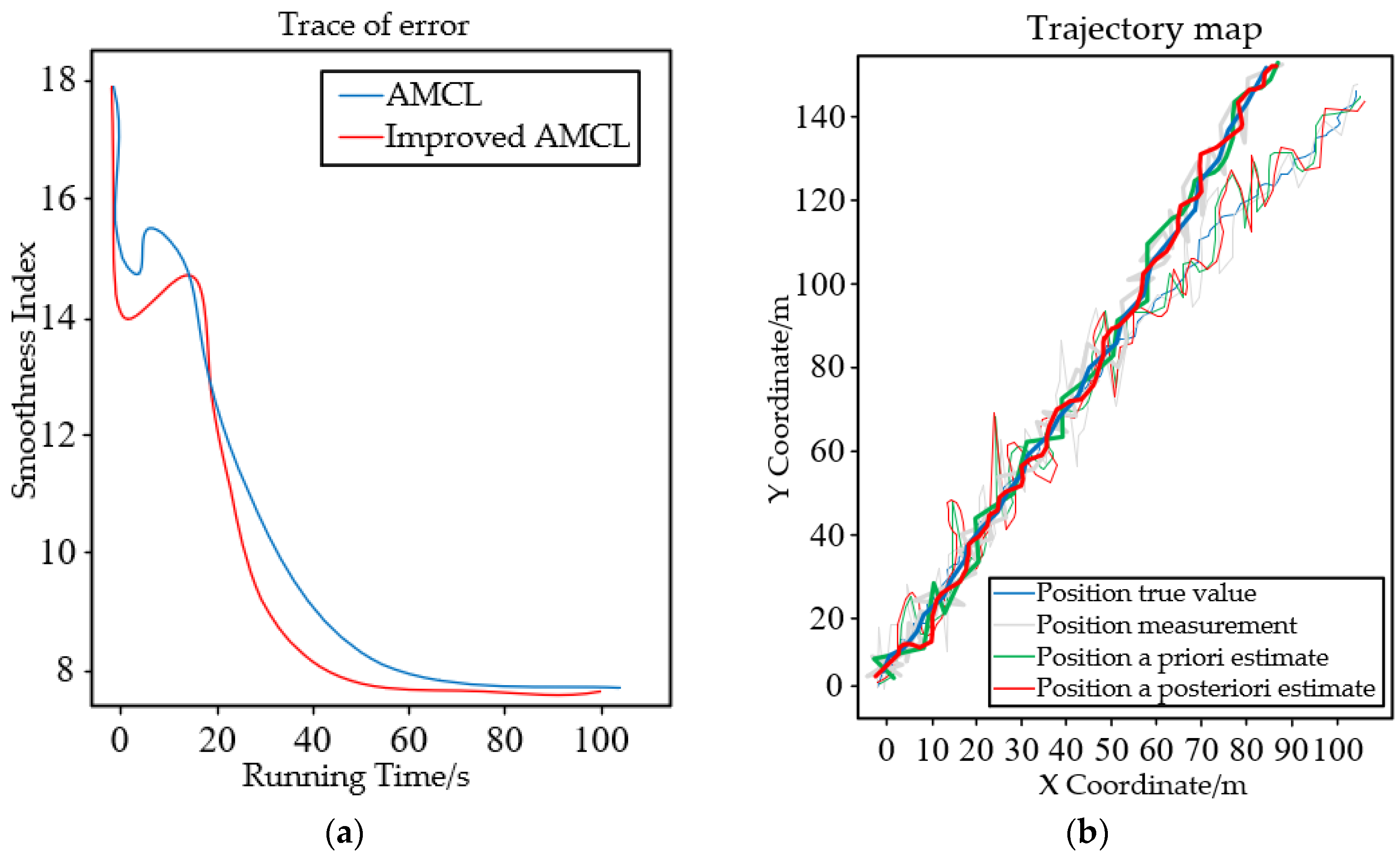
Improving the generation of the initial particle swarm can improve the convergence speed and accuracy of the algorithm, and improve the resampling method to effectively reduce or avoid the kidnapping problem. By building the simulation model and testing the simulation using MATLAB software, the algorithm can be made to converge faster and more accurately to the AGV position, as well as improving the real-time and responsiveness of the system, and greatly reducing the time required for navigation.

4

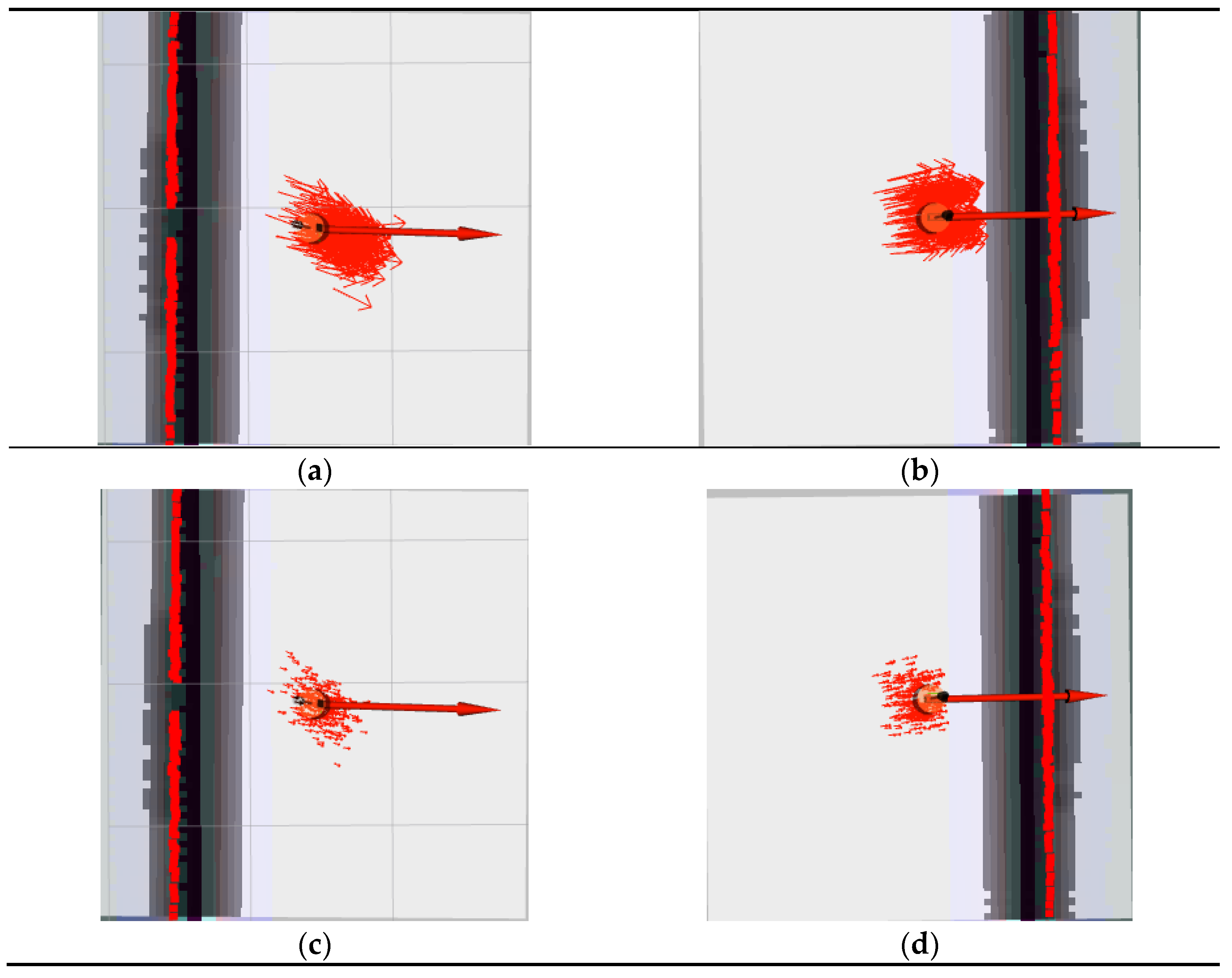
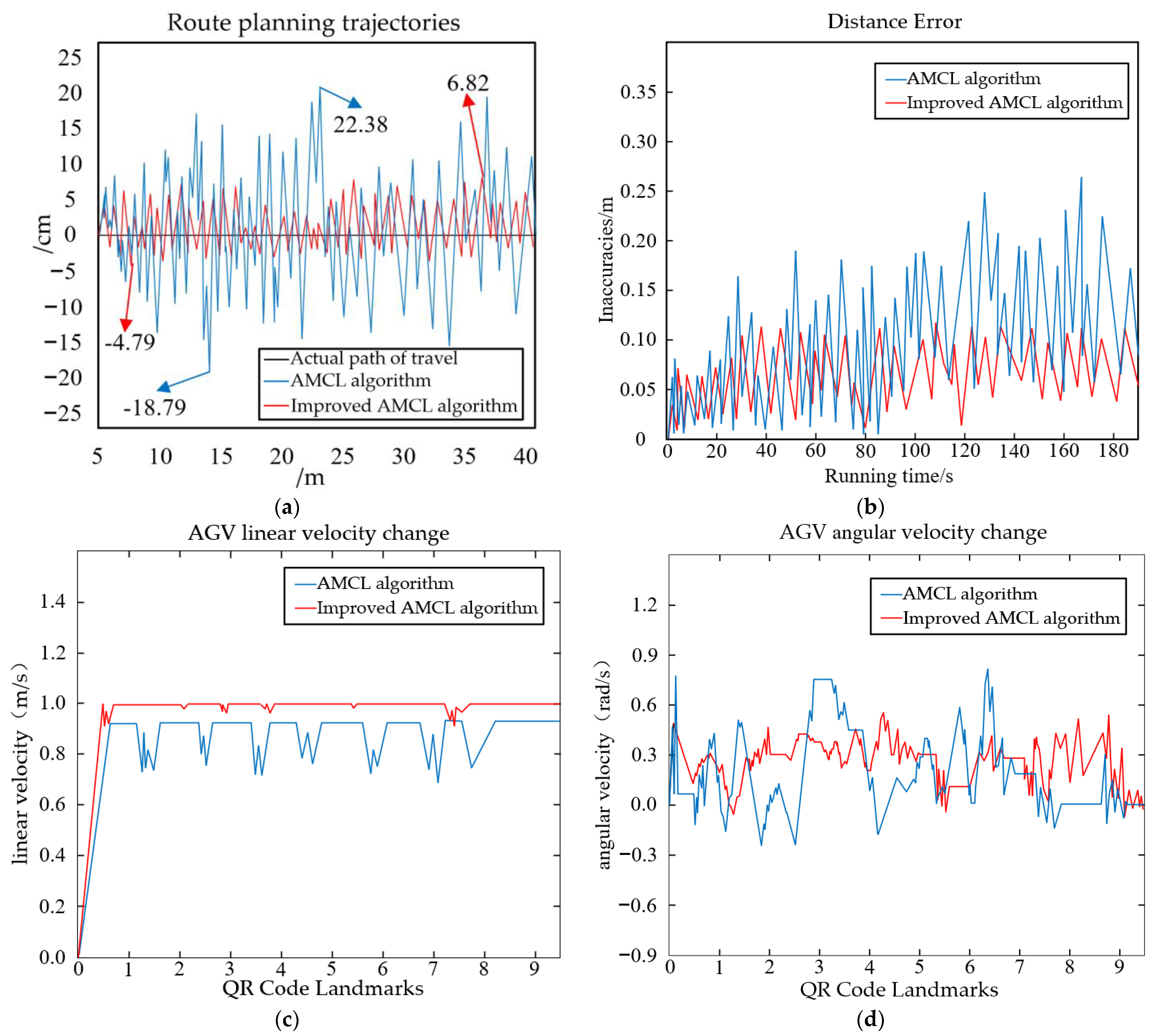
When the particles generated by the AMCL algorithm encounter the kidnapping situation, i.e., the AGV generates too much offset and the particle state does not change with the movement of the AGV. Through comparison, it can be learnt that the improved AMCL algorithm can quickly adjust the attitude and correct the offset distance, so that it can quickly return to the original travelling route, and the resumption of the adjustment time has been improved by 68.73% compared with the unimproved algorithm.

5

During AGV navigation, the time required for navigation was reduced by 42.81% compared to the unimproved algorithm. The navigation time is greatly reduced, which speeds up the time to process the goods and improves the turnaround speed and capacity of the goods. The positioning accuracy is an important criterion to measure the accuracy of the proposed algorithm. In this paper, by comparing and contrasting, it is concluded that the positioning accuracy is improved by 64.27% compared to the previous algorithm.

In the following research, we will pay more attention to the accuracy and practicality of AGVs in positioning and navigation. For example, we will study the practical application of visual navigation in AGVs and further combine visual information with or instead of QR code data to improve the ability of AGVs to sense their surroundings. In addition, we aim to make a major breakthrough in visual autonomous navigation in AGVs, i.e., to achieve more accurate positioning and no interference throughout the autonomous navigation process, and to apply it to more complex operational tasks and environments.

References

- Cheng, W.; Chen, J.; Yang, L.; Li, Z.; Zhou, Y. Optimization design and implementation of automatic guided vehicle. J. Hunan Inst. Technol. Nat. Sci. Ed. 2021, 34, 45–49. (In Chinese) [Google Scholar]
- Bechtsis, D.; Tsolakis, N.; Vlachos, D.; Iakovou, E. Sustainable supply chain management in the digitalisation era: The impact of Automated Guided Vehicles. J. Clean. Prod. 2017, 142, 3970–3984. [Google Scholar] [CrossRef]
- Okumuş, F.; Kocamaz, A.F. Cloud Based Indoor Navigation for ROS-enabled Automated Guided Vehicles. In Proceedings of the 2019 International Artificial Intelligence and Data Processing Symposium (IDAP), Malatya, Turkey, 21–22 September 2019; pp. 1–4. [Google Scholar]
- Li, Y. Research on Multi-AGVs Cooperative Transportation Strategy in Warehouse Logistics Environment Based on HCA Algorithm. In Proceedings of the 2023 IEEE 2nd International Conference on Electrical Engineering, Big Data and Algorithms (EEBDA), Changchun, China, 24–26 February 2023; pp. 1753–1758. [Google Scholar] [CrossRef]
- Li, W.; Zhang, N.; Yao, Y.; Zhan, H.; Ding, Y. Research on Vision Navigation and Positioning of AGV Terminal Based on QR Code. In Proceedings of the 2020 IEEE 9th Joint International Information Technology and Artificial Intelligence Conference (ITAIC), Chongqing, China, 11–13 December 2020; pp. 845–848. [Google Scholar] [CrossRef]
- Zhang, B.; Zhu, M.; Lin, C.; Zhu, D. Research on AGV map building and positioning based on SLAM technology. In Proceedings of the 2022 IEEE 5th International Conference on Automation, Electronics and Electrical Engineering (AUTEEE), Shenyang, China, 18–20 November 2022; pp. 707–713. [Google Scholar] [CrossRef]
- Bach, S.H.; Khoi, P.B.; Yi, S.Y. Application of QR Code for Localization and Navigation of Indoor Mobile Robot. IEEE Access 2023, 11, 28384–28390. [Google Scholar] [CrossRef]
- Kulaç, N.; Engin, M. Developing a Machine Learning Algorithm for Service Robots in Industrial Applications. Machines 2023, 11, 421. [Google Scholar] [CrossRef]
- Kumar, P.; Khaparde, A. QR Code Detector and Follower with Kalman Filter. In Proceedings of the 2022 International Interdisciplinary Humanitarian Conference for Sustainability (IIHC), Bengaluru, India, 18–19 November 2022; pp. 1423–1426. [Google Scholar] [CrossRef]
- Zhou, C.; Liu, X. The Study of Applying the AGV Navigation System Based on Two Dimensional Bar Code. In Proceedings of the 2016 International Conference on Industrial Informatics—Computing Technology, Intelligent Technology, Industrial Information Integration (ICIICII), Wuhan, China, 3–4 December 2016; pp. 206–209. [Google Scholar] [CrossRef]
- Talwar, D.; Jung, S. Particle Filter-based Localization of a Mobile Robot by Using a Single Lidar Sensor under SLAM in ROS Environment. In Proceedings of the 2019 19th International Conference on Control, Automation and Systems (ICCAS), Jeju, Republic of Korea, 15–18 October 2019; pp. 1112–1115. [Google Scholar] [CrossRef]
- Zhang, X.; Mu, X.; Liu, H.; He, B.; Yan, T. Application of Modified EKF Based on Intelligent Data Fusion in AUV Navigation. In Proceedings of the 2019 IEEE Underwater Technology (UT), Kaohsiung, Taiwan, 16–19 April 2019; pp. 1–4. [Google Scholar] [CrossRef]
- Trisnawan, I.K.N.; Jati, A.N. Monte Carlo method is a kind of calculation method, but it is very different from the general numerical calculation method, it is based on the theory of probability statistics. In Proceedings of the 2019 International Conference on Computer, Control, Informatics and its Applications (IC3INA), Tangerang, Indonesia, 23–24 October 2019; pp. 187–192. [Google Scholar]
- dos Reis, W.P.N.; Morandin, O.; Vivaldini, K.C.T. A Quantitative Study of Tuning ROS Adaptive Monte Carlo Localization Parameters and their Effect on an AGV Localization. In Proceedings of the 2019 19th International Conference on Advanced Robotics (ICAR), Belo Horizonte, Brazil, 2–6 December 2019; pp. 302–307. [Google Scholar] [CrossRef]
- Zeghmi, L.; Amamou, A.; Kelouwani, S.; Boisclair, J.; Agbossou, K. A Kalman-Particle Hybrid Filter For Improved Localization of AGV In Indoor Environment. In Proceedings of the 2022 2nd International Conference on Robotics, Automation and Artificial Intelligence (RAAI), Singapore, Singapore, 9–11 December 2022; pp. 141–147. [Google Scholar] [CrossRef]
- Zou, Q. Research on Mobile Robot Navigation Method Based on Graph Optimization SLAM. Master’s Thesis, Harbin Institute of Technology, Harbin, China, 2017. (In Chinese). [Google Scholar]
- Zhang, F.; Li, S.; Yuan, S.; Sun, E.; Zhao, L. Algorithms analysis of mobile robot SLAM based on Kalman and particle filter. In Proceedings of the 2017 9th International Conference on Modelling, Identification and Control (ICMIC), Kunming, China, 10–12 July 2017; pp. 1050–1055. [Google Scholar] [CrossRef]
- Kumar NT, S.; Gawande, M.; M, N.P.B.; Verma, H.; Rajalakshmi, P. Mobile Robot Terrain Mapping for Path Planning using Karto Slam and Gmapping Technique. In Proceedings of the 2022 IEEE Global Conference on Computing, Power and Communication Technologies (GlobConPT), New Delhi, India, 23–25 September 2022; pp. 1–4. [Google Scholar] [CrossRef]
- Chung, M.-A.; Lin, C.-W. An Improved Localization of Mobile Robotic System Based on AMCL Algorithm. IEEE Sens. J. 2022, 22, 900–908. [Google Scholar] [CrossRef]
- Tiwari, S. An Introduction to QR Code Technology. In Proceedings of the 2016 International Conference on Information Technology (ICIT), Bhubaneswar, India, 22–24 December 2016; pp. 39–44. [Google Scholar] [CrossRef]
- Cui, G.; Bai, Y.; Li, S. AGV Research Based on Inertial Navigation and Vision Fusion. In Proceedings of the 2021 5th CAA International Conference on Vehicular Control and Intelligence (CVCI), Tianjin, China, 29–31 October 2021; pp. 1–6. [Google Scholar] [CrossRef]
- Zheng, Z.; Yu, Y.; Chen, R.; Huang, H.; Zhao, H.; Lu, X. Localization Method Based on Multi-QR Codes for Mobile Robots. In Proceedings of the 2022 IEEE International Conference on Advances in Electrical Engineering and Computer Applications (AEECA), Dalian, China, 20–21 August 2022; pp. 1385–1391. [Google Scholar] [CrossRef]
- Li, Z.; Huang, J. Study on the use of Q-R codes as landmarks for indoor positioning: Preliminary results. In Proceedings of the 2018 IEEE/ION Position, Location and Navigation Symposium (PLANS), Monterey, CA, USA, 23–26 April 2018; pp. 1270–1276. [Google Scholar] [CrossRef]
- Xia, L.; Cui, J.; Shen, R.; Xu, X.; Gao, Y.; Li, X. A Survey of Image Semantics-based Visual Simultaneous Localization and Mapping: Application-oriented Solutions to Autonomous Navigation of Mobile Robots. Int. J. Adv. Robot. Syst. 2020, 17, 4158. [Google Scholar] [CrossRef]
- Balasuriya, B.; Chathuranga, B.; Jayasundara, B.; Napagoda, N.; Kumarawadu, S.; Chandima, D.; Jayasekara, A. Outdoor robot navigation using Gmapping based SLAM algorithm. In Proceedings of the 2016 Moratuwa Engineering Research Conference (MERCon), Moratuwa, Sri Lanka, 5–6 April 2016; pp. 403–408. [Google Scholar] [CrossRef]
- Su, Z.; Zhou, J.; Dai, J.; Zhu, Y. Optimization Design and Experimental Study of Gmapping Algorithm. In Proceedings of the 2020 Chinese Control And Decision Conference (CCDC), Hefei, China, 22–24 August 2020; pp. 4894–4898. [Google Scholar] [CrossRef]
- Zhou, H.; Chou, W.; Tuo, W.; Rong, Y.; Xu, S. Mobile Manipulation Integrating Enhanced AMCL High-Precision Location and Dynamic Tracking Grasp. Sensors 2020, 20, 6697. [Google Scholar] [CrossRef] [PubMed]
- Qi, X.; Ji, W.; Wang, Q. A Monte Carlo localization Algorithm based on Ranging. In Proceedings of the 2019 3rd International Conference on Electronic Information Technology and Computer Engineering (EITCE), Xiamen, China, 6–8 November 2019; pp. 1663–1666. [Google Scholar] [CrossRef]
- Zhang, H.; Sun, C.-L.; Zeng, Y.-M.; Li, P.-P. A Fusion Localization Algorithm Combining MCL with EKF. In Proceedings of the 2018 17th International Symposium on Distributed Computing and Applications for Business Engineering and Science (DCABES), Wuxi, China, 19–23 October 2018; pp. 216–220. [Google Scholar] [CrossRef]
- Dong, S.; Lin, R.; Zhao, W.-W.; Cheng, Y.-H. Robot Global Relocalization Based on Multi-sensor Data Fusion. In Proceedings of the 2022 2nd International Conference on Robotics, Automation and Artificial Intelligence (RAAI), Singapore, Singapore, 9–11 December 2022; pp. 35–42. [Google Scholar] [CrossRef]