DP-YOLO: Effective Improvement Based on YOLO Detector

Abstract

YOLOv5 remains one of the most widely used real-time detection models due to its commendable performance in accuracy and generalization. However, compared to more recent detectors, it falls short in label assignment and leaves significant room for optimization. Particularly, recognizing targets with varying shapes and poses proves challenging, and training the detector to grasp such features requires expert verification or collective discussion during the dataset labeling process, especially in domain-specific contexts. While deformable convolutions offer a partial solution, their extensive usage can enhance detection capabilities but at the expense of increased computational effort. We introduce DP-YOLO, an enhanced target detector that efficiently integrates the YOLOv5s backbone network with deformable convolutions. Our approach optimizes the positive sample selection during label assignment, resulting in a more scientifically grounded process. Notably, experiments on the COCO benchmark validate the efficacy of DP-YOLO, which utilizes an image size of [640, 640], achieves a remarkable 41.2 AP, and runs at an impressive 69 fps on an RTX 3090. Comparatively, DP-YOLO outperforms YOLOv5s by 3.2 AP, with only a small increase in parameters and GFLOPSs. These results demonstrate the significant advancements made by our proposed method.

1. Introduction

Computer vision uses computer technology to process and analyze digital images and videos. Deep learning has significantly advanced object detection, a fundamental task in this field. Its widespread use spans various industries, including autonomous driving, security monitoring, industrial manufacturing, medical diagnosis, retail, and agriculture, due to improved accuracy and efficiency.

Object detection algorithms can be broadly categorized into two types: Two-stage algorithms [1,2,3] that involve candidate region extraction and classifier prediction, and one-stage algorithms [4,5,6] that combine feature extraction and target classifier prediction directly. Among single-stage algorithms, the YOLO family, particularly YOLOv5, balanced accuracy, speed, ease of training, and deployment. In addition to its excellent scalability resulting from the integration of numerous tricks and modularized code, YOLOv5 also provides lighter versions. But we are still in the predicament that although the detection ability of large CNN [7] or transformer [8,9]-based detection algorithms is very close to human or even beyond, their huge computational cost makes it difficult to be widely used in production and life. The vision tasks will be oriented to both the colorful nature and also be applied to some special situations in specific domains, which puts a higher demand on detectors with less computational resource consumption. When we apply YOLOv5 and other algorithms trained on generalized datasets to domain-specific datasets, some limitations arise, including poor detection of small targets, insufficient adaptation to complex backgrounds, and limited ability to deal with target deformation and attitude changes. Addressing these issues while maintaining the algorithm’s efficiency has emerged as a critical focus in object detection.

While domain-specific dataset detection targets are not used for a myriad of possibilities as are silhouettes of human activity and nature, most of them have unique image characteristics in addition to often being characterized by limited data and category imbalance. For instance, microscopic images of urine sediment lack prominent features visible to the human eye. Additionally, such datasets exhibit an increased number of small targets, category confusion, and significant morphological and gestural differences within similar categories. To enhance detection accuracy in these complex and specific scenarios, this paper builds upon the YOLOv5 detection framework by incorporating deformable convolutions into the backbone network more efficiently. Furthermore, improvements are made in the label assignment strategy, and the proposed method’s effectiveness is validated in detecting these distinct images.

The contributions of our work can be listed as follows:

• Modifying the expansion policy of positive samples in label assignment. Combined with the previous work, the quality of positive samples can be improved by considering the effective receptive field characteristics, which can be used to update the parameters in the deep network to obtain a better detector.
• Introducing deformable convolution into the backbone network of YOLOv5s in a more cost-effective way. By leveraging the distinct properties of various deformable convolution operators to design and balance them, a substantial enhancement in detection accuracy is attained on the generalized dataset. Remarkably, this improvement is achieved with only a minor increase in the number of parameters and computational effort required.
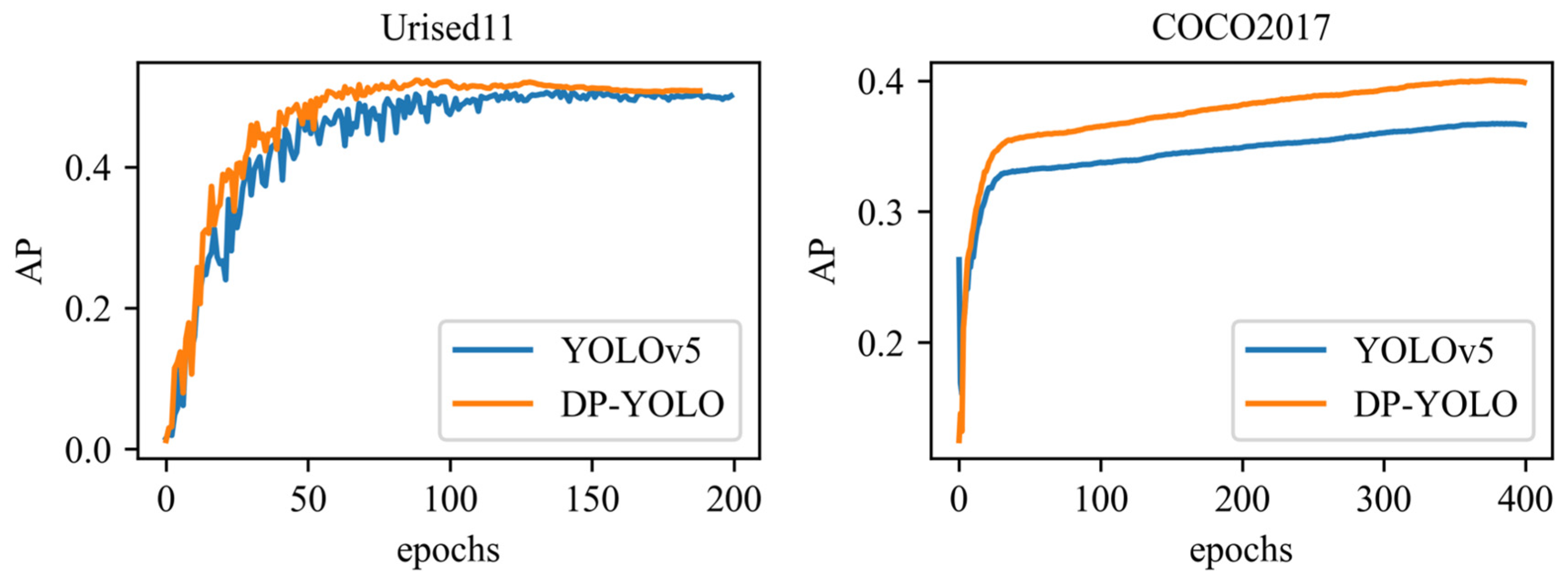
• The improved detector DP-YOLO under the action of both methods was validated and analyzed on a urine sediment dataset for a specific assay domain, in addition to being validated on the generic dataset COCO2017.

2. Related Work

2.1. Label Assignment

Label assignment is a critical process in the training stage of a detection model. It involves distinguishing between positive and negative samples and assigning appropriate learning targets to each position on the feature map, shaping how the model learns and converges. In the case of anchor-based detectors, the IoU (intersection over union) between anchors and ground truth is a pivotal criterion for this task. Traditionally, two or three fixed thresholds are employed to define positive and negative samples. Each anchor’s IoU with all ground truth is calculated, designating anchors above the higher IoU threshold as positive samples and those below the lower threshold as negatives. Additionally, the anchor position with the highest IoU among all anchors is considered a positive sample for each ground truth if the IoU exceeds the minimum threshold. Other anchors are ignored during training and do not participate in the network’s gradient update. As an illustration, Faster R-CNN [3] employs this strategy along with a random sampling of anchors to train its RPN and R-CNN modules. Building on Faster R-CNN, Libra R-CNN [10] enhances the sampling method with a more scientifically grounded approach. On the other hand, RetinaNet [6] does not use any sampling and instead relies on two distinct and strict thresholds for positive and negative samples. These thresholds ensure that each ground truth has precisely one positive sample assigned. Regarding Anchor-free detection algorithms, FCOS [11] determines sample matching based on whether the sample point falls within the center region of the ground truth. Moreover, it utilizes different regression ranges at various FPN feature layers. On the other hand, CenterNet [12] relies on the center point of the ground truth and introduces a Gaussian heatmap to determine positive and negative samples.

In recent years, there has been an increasing emphasis on adaptive strategies for label assignment in object detection. Notably, FreeAnchor [13], ATSS [14], OTA [15], AutoAssign [16], etc., have made significant contributions in this direction. FreeAnchor employs a loss function that eliminates the manual specification of anchors. It utilizes maximum likelihood estimation, enabling the network to autonomously learn to select anchors that best match the ground truth. ATSS introduces adaptive training sample selection by calculating the mean and variance of the IoU between candidate boxes of positive samples and ground truth. This approach dynamically determines IoU thresholds for dividing positive and negative samples. The OTA algorithm formulates the label assignment process as an optimal transport problem, leveraging global information to find the optimal sample-matching strategy and thereby improving accuracy. AutoAssign, based on FCOS, takes a completely data-driven approach by dynamically matching positive and negative samples without prior knowledge, making the label assignment process more flexible and adaptable. On the other hand, TAL (task alignment learning) [17] focuses on bringing the optimal anchors of classification and regression tasks closer together. This is achieved by designing a sample allocation strategy and a task alignment loss, which work together to gradually unify the optimal anchors of classification and localization tasks. The goal of TAL is to enhance the overall performance of the detector.

During the evolution of the YOLO series, significant variations have occurred in its label assignment approach. In YOLOv1 [4], the IoU between the two bounding boxes of the grid containing the center point of the ground truth is calculated, and the larger bounding box is considered a positive sample. In YOLOv2 [18] and YOLOv3 [19], the label assignment is similar to RetinaNet, ensuring each ground truth has a unique positive sample. Due to YOLO’s nature, the anchor considered must belong to the grid containing the center point of the ground truth. In YOLOv3, multi-scale prediction is employed across different prediction layers, while YOLOv4 [20] takes a different approach and treats all anchors as positive samples as long as they surpass the IoU threshold. Furthermore, Zheng et al. simplified the sample assignment strategy of OTA and introduced SimOTA to achieve a balance between positive and negative samples [21]. SimOTA utilizes a Top-K approximation strategy, which involves using the IoU values of ground truth and anchors with the loss matrix to find the best match of samples. This approach significantly accelerates the training process and has been successfully applied in YOLOX [21]. Subsequently, it has also been implemented in YOLOv7 [22] detectors. Moreover, in YOLOv6 [23], a comparison was made between SimOTA and TAL, and it was concluded that TAL is more effective in stabilizing training and improving detection performance.

The YOLOv5 detection algorithm utilizes a label assignment approach that matches and filters anchors based on shape (i.e., the extremes of width-to-height ratios) across multiple detection layers. Additionally, the algorithm augments positive samples through a cross-grid expansion strategy, thereby enhancing the network’s ability to learn and detect targets effectively. This static label assignment method has proven to achieve impressive detection accuracy and generalizability within its detection framework at that time. But now, its positive impact on training compared to the latest dynamic matching strategies needs to be further extended. For other label assignments, some of them, such as FreeAnchor [13], ATSS [14], TAL [17], and OTA [15], may introduce complexity to the process and slow down the training; some are incompatible with anchor-based detectors that possess the concept of grid, such as AutoAssign [16] and SimOTA [21].

2.2. Deformable Convolution

The conventional convolution operation involves dividing the feature map into rectangles of the same size as the convolution kernel and performing the convolution. In contrast, group convolution groups the number of channels and uses different convolution kernels for each group, reducing the number of parameters and making the network more lightweight. Depth-separable convolution splits the convolution process into depth-wise convolution and point-wise convolution, further optimizing the number of convolution parameters. Dilated convolution introduces dilation rates to increase the receptive field of the convolution operation. However, these operations still perform convolution on an N × N grid, resulting in a theoretical receptive field that is close to a rigid square, not adequately capturing the actual shape of objects. To address this limitation, Dai et al. [24] proposed DCN (Deformable Convolution), which introduces a learnable offset to the sampling position of the convolution. This deformation makes the receptive field adaptive to geometric changes, allowing for more accurate feature extraction and enhancing the network’s adaptability to various deformations.

Zhu et al. [25] raised concerns about the introduction of irrelevant contextual information in DCN due to the offset module. To address this, they proposed DCNv2, which incorporates new learnable weights into the deformable convolution. This modification helps mitigate the interference of irrelevant factors during model training. They demonstrated that DCNv2 layers, when applied more extensively in the backbone network, enhance the network’s ability to model geometric transformations effectively. On the other hand, Wang et al. [26] initiated their work with the concept of constructing a large-scale vision base model. Drawing insights from DCNv2 and taking inspiration from MHSA [8] along with depth-separable convolution, they devised a more lightweight deformable convolution known as DCNv3. Implementing DCNv3 in their approach called InternImage, achieves a state-of-the-art level in the detection task at the time.

Due to the diversity of visual task objectives, it is important for models to have deformational representations, and adding deformable convolution to the network to improve performance is a viable means of doing so, but it is more worthwhile to explore how to achieve more efficient utilization.

3. Approaches

We devised two tricks to improve the detection accuracy of YOLOv5: incorporating deformable convolution into the backbone network and refining the label assignment strategy for samples. Figure 1 illustrates the framework of our approach. The introduction of appropriate deformable convolutions enhances the adaptability of the backbone network to accommodate diverse morphologies and poses of targets within images, and this advancement leads to improved detection results, particularly for categories exhibiting significant variations and challenging features. Simultaneously, the optimized label assignment provides more suitable learning targets for the model, ultimately resulting in higher detection accuracy. These combined improvements enhance the overall effectiveness and efficiency of the YOLOv5.

3.1. Petal-like Sample Amplification (PSA)

The sample matching method of YOLOv5 involves two stages. In the former stage, each detection layer has three anchors of different sizes for every grid. For each ground truth, the ratio of its length to width is calculated with different anchors, and if the ratio falls within the specified threshold range of 0.25–4, the associated anchor is considered a positive sample. The grid where the center point is located is also treated as a positive sample, and its own confidence loss is calculated. Additionally, when the centroid of the ground truth falls into a different region of the grid, the associated anchor of the corresponding adjacent grid will also be expanded as a positive sample. As shown in Figure 2, the center points of the ground truth represented by the red, orange, green, and white dots are located in the upper right corner area of their respective grids. Therefore, the associated anchors of the grid above and to the right will also be considered positive samples, as depicted in the three gray boxes in the figure. This process expands the positive samples twice for each case.

We firmly advocate for sample augmentation across grids to be conducted within the appropriate range. Previous studies have utilized a solid circle centered at the object’s center to define positive samples [27]. Moreover, it has been observed that pixels within the theoretical receptive field contribute to the output cell with an asymptotically Gaussian distribution [28]. Integrating the circle-like characteristics of the effective receptive field into the sample selection process would further enhance the quality of positive samples [29]. By incorporating these insights, the sample should be expanded into the positive sample because it can ‘feel’ the ground truth. Specifically, we draw a circle with the centroid of each grid as the center and a certain length as the radius. If the centroid of the ground truth lies within this circle, the associated anchors of that grid are expanded into positive samples, and this approach resembles the effective receptive field concept. Since the expanded ranges of multiple neighboring grids will form a shape similar to two petals when they overlap, we named it Petal-like Sample Amplication (PSA).

3.2. Deformable YOLO v5 Backbone (DYB)

Currently, in many detection algorithms, the backbone network employs blocks of different sizes for feature extraction and processing at each downsampling stage. To enhance the detection performance of YOLOv5 further, we introduce a crucial modification in the backbone network. Specifically, we replace the normal convolution used in the bottleneck structure of the C3 module of the YOLOv5s backbone network with a deformable convolutional operator. The modification is depicted in Figure 3, and we carefully consider the trade-off between accuracy and efficiency. We incorporate the deformable convolutional operator at different downsampling stages of the YOLOv5s backbone, as illustrated in Figure 4.

In our approach, we have designed two modules, namely D2C3 and D3C3, taking inspiration from the characteristics of the deformable convolution operators DCNv2 and DCNv3, respectively. These modules are applied to the backbone network of YOLOv5 to improve its detection performance. The D2C3 module utilizes the DCNv2 deformable convolution operator, which has innumerable parameters. It employs separate projection weights for each sampling point’s feature vector. On the other hand, the D3C3 module incorporates the DCNv3 deformable convolution operator, which is more lightweight. By introducing grouped convolution, D3C3 becomes better suited to handle network levels with a larger number of channels in the tensor. The design of these two modules allows us to effectively leverage the strengths of DCNv2 and DCNv3 deformable convolution operators to enhance the backbone network’s feature extraction capabilities.

Table 1. Cost of different downsampling phases for three blocks in YOLO v5s backbone network.

	Stage 1		Stage 2		Stage 3		Stage 4
	$\mathbf{Params}$	$\mathbf{GFLOPs}$	$\mathbf{Params}$	$\mathbf{GFLOPs}$	$\mathbf{Params}$	$\mathbf{GFLOPs}$	$\mathbf{Params}$	$\mathbf{GFLOPs}$
C3	18.8 K	31.5	115.7 K	47.8	625.2 K	64.3	1.4 M	21.6
D2C3	50.1 K	67.3	240.5 K	68.6	999.1 K	57.2	1.2 M	30.4
D3C3	16.7 K	16.7	96.6 K	39.9	503.2 K	51.7	1.0 M	26.1

shows the cost of the different downsampling stages in the backbone network of YOLOv5s for three modules: C3, D2C3, and D3C3. The number of groupings for the DCNv3 operator in the D3C3 module is set to the same value as in InternImage [26], which is determined by dividing the number of tensor channels it processes by 16. The computation cost is simulated for each stage using an input size of 640 × 640 × 3. The comparison of these costs allows us to assess the efficiency and performance of the different modules in the backbone network of YOLOv5s.

3.3. Urine Sediment Dataset

As the COCO dataset poses challenges due to its large number of categories and images, we opted to conduct further validation of our method on the Urised11 urinary sediment dataset. The Urised11 dataset is a subset of the Urised2022 dataset, sourced from the Hefei Institute of Physical Sciences of the Chinese Academy of Sciences. The Urised11 dataset comprises 7364 images and includes 11 categories with a total of 58,196 labeled instances.

3.3.1. Urine Sediment Detection

Urine sediment detection plays a crucial role in clinical pathology, particularly in evaluating renal, urologic, metabolic, and diabetic disorders. It involves the microscopic examination of a urine sample to analyze the density and number of cells, crystals, and other particles present. The interpretation of urine sediment composition provides valuable information about underlying diseases. For instance, the presence of red blood cells or a tubular pattern may indicate glomerular disease, while the presence of white blood cells may indicate infection or inflammation, and the presence of crystals may suggest metabolic disorders, among other possibilities. Traditionally, this examination process has been manually conducted by experienced professionals. However, this approach is time-consuming, labor-intensive, subject to inaccuracies, and prone to subjective human errors. In previous years, researchers have explored the use of traditional machine learning algorithms in automating this process, and despite these efforts, achieving accurate and efficient results suitable for practical clinical use remains a challenge.

Indeed, the advent of deep-learning-based target detection techniques has opened up promising possibilities for automating the urine sediment detection process. Researchers have made notable strides in this area, demonstrating the potential of deep learning in this specialized domain. For instance, Liang et al. [30] introduced a multi-view residual model that achieved significant advancements in automated urine sediment detection on their self-constructed USE dataset. This work showcased the power of deep learning in efficiently analyzing urine sediment compositions and extracting valuable information from microscopic images. Additionally, Avci et al. [31] applied innovative super-resolution and denoising image processing techniques to further enhance urinary sediment detection. Their approach demonstrated how combining deep learning with sophisticated image processing methods can lead to improved accuracy and reliability in detecting and analyzing urinary sediment samples.

3.3.2. Datasets in the Field of Urine Sediment Detection

Microscopic images of urinary sediment are obtained by placing the urine sample on a slide and examining it under a microscope after centrifugal precipitation to separate out the urinary sediment. However, labeling these images presents challenges due to the characteristics of optical blurring, cellular overlap, low contrast, and small cell size. Furthermore, detecting the observable components of these images is also notably difficult, adding to the complexity of targeting detection.

The majority of publicly available datasets for urinary sediment exhibit limited quantities of images, and their labeling lacks uniformity and standardization. However, with the increasing prevalence of computer vision applications in urine sediment detection in recent years, there has been a surge in the development of new object detection datasets. These datasets aim to address the shortcomings of the earlier collections and provide more comprehensive and standardized resources for the advancement of this field. Dipam’s UMID (urine sediment microscopic image) dataset comprises 366 images with a total of 3.733 k labels, including three types: RBC, pus, and epithelial cells [32]. Liang’s USE dataset contains 5.377 k images with 42.759 k labels, categorized into seven classes: Cast, cryst, epith, epithn, eryth, leuko, and mycete [30]. Recently, Tuncer et al. acquired urine images from 409 patients from hospital applications, resulting in 8509 instances covering 8 categories: Erythrocyte, Leukocyte, Epithelial, Bacteria, Yeast, Cylinders, Crystals, and others (sperms, etc.) [33].

3.3.3. Urised11

The Urised11 dataset is an extensive collection of 7.364 k microscopic images of urinary deposits, each sized 720 × 576 pixels, containing a total of 58.196 k labels. The dataset encompasses 11 distinct categories: Erythrocytes (eryth), leukocytes (leuko), leukocyte clusters (leukoc), squamous epithelial cells (epith), non-squamous epithelial cells (epithn), cast, pathological cast (pcast), spermatozoa (sperm), yeast (yeast), mycete/bacteria (mycete), and crystals (cryst). Hence, it is aptly named Urised11. To facilitate training and evaluation, the Urised11 dataset is partitioned into a 4:1 ratio, with 5891 images allocated to the training dataset and 1473 images to the evaluation dataset. According to the number of labels in Urised11 in

Table 2. Overview of Urised11.

Classes	Sample	Train Labels	Val Labels	Classes	Sample	Train Labels	Val Labels
eryth		22,731	6065	cast		2673	646
leuko		6171	1525	pcast		717	205
leukoc		573	153	epith		7035	1562
mycete		939	227	epithn		336	117
cryst		2605	664	sperm		108	25
yeast		2560	559

, we can see that the number of labels in each category roughly matches the 4:1 ratio.

There are significant variations among the components of the same class in Urised11. Among them, seven components exhibit substantial differences, and we have listed them in

Table 3. Seven categories with large variations in Urised11.

Class	LPIPS	Samples
epith	0.505
pcast	0.497
sperm	0.496
cast	0.474
mycete	0.415
epithn	0.407
yeast	0.396

. To assess the similarity of images belonging to each class of urinary sediment components, we utilized the AlexNet [34] deep convolutional network in conjunction with the perceptual metric LPIPS (Learned Perceptual Image Patch Similarity) [35]. The LPIPS value represents the average image-perceived similarity between two instances of 100 randomly selected image examples from each class of components, effectively indicating the intra-class similarity of the urinary sediment components within that specific class. Higher LPIPS values indicate greater intra-class variation among these images. Notably, the source of the Urised11 dataset’s images stems from the observation of urinary sediment precipitated after centrifugal sedimentation. As a result, its target background exhibits less variability compared to that of the COCO2017 dataset. Consequently, the intra-class differences primarily stem from the target’s deformation and pose changes.

The urine sediment dataset we used has only 11 categories, which is not sufficiently comprehensive in terms of the classes of urine sediment. But the Urised11 dataset is sufficient to validate the performance of the assay in this field. The content of this work is still being continuously updated, and the next step will be to expand and refine the assay types to 36 observable components of urinary sediment, which can better fulfill the practical needs in this field.

4. Experiment

4.1. Experimental Environment and Details

Our experiments were conducted on a DELL PowerEdge 640 server equipped with four GeForce RTX 3090 GPUs (24GB memory). The software environment utilized for the experiments included Ubuntu 20.04, CUDA 11.2, Python 3.9, and PyTorch 1.12.1. During training, we employed the SGD optimizer, selecting the CIoU Loss as the bounding box regression loss, with a batch size of 64 per graphics card. We followed the default configuration of YOLOv5, setting the initial learning rate to 0.01, learning rate decay to 0.0005, running the training for 300 epochs, and using an input image size of 640 × 640. We trained and evaluated our method on the COCO2017 dataset [36] and VOC07 + 12(see Appendix A). Additionally, we conducted a comparative analysis between our method and other SOTA (state-of-the-art) detection methods using the Urised11 dataset. For fairness, the other SOTA (state-of-the-art) detection methods were standardized within the MMDetection [37] toolbox.

4.2. Evaluation Metrics

The more common evaluation metrics in object detection are accuracy (Precision), recall (Recall), average precision (AP), parameters, FLOPs and frames per second (FPS). The specific formulas are as follows:

$$Precision\left(P\right)=\frac{TP}{TP+FP}$$

$$Recall\left(R\right)=\frac{TP}{TP+FN}$$

$$AP=\frac{1}{n}\sum _{i=1}^n{\int }_0^{1}P\left(R\right)dR$$

where $TP$ (true positive) means the sample is correctly classified as positive; $FP$ (false positive) means the sample is incorrectly classified as positive; $FN$ (false negative) means the sample is incorrectly classified as negative; $n$ denotes the number of categories; and $AP$ is the average value of area under the PR curve for each category.

In this paper, the COCO [36] criterion was adopted using pycocotools tool implementation. $AP$ (average of mean accuracies with IoU within [0.5:0.95]), ${AP}_{50}$ (mean accuracy with IoU threshold of 0.50), ${AP}_{75}$ (mean accuracy with IoU threshold of 0.75), ${AP}_s$ (mean accuracy for small targets), ${AP}_m$ (mean accuracy for medium targets) and ${AP}_l$ (mean accuracy for large targets) are used as the evaluation metrics. Params are used to measure the size of the model, FLOPs describe the complexity of the algorithm, and FPS indicates how many images can be processed per second.

4.3. Experimental Results and Analysis

Table 4. Comparison experiments on COCO2017.

Method	$\mathbf{\#}\mathbf{Params}$	$\mathbf{GFLOPs}$	FPS	$\mathit{A}\mathit{P}$	${\mathit{A}\mathit{P}}_{50}$	${\mathit{A}\mathit{P}}_{75}$	${\mathit{A}\mathit{P}}_{\mathit{s}}$	${\mathit{A}\mathit{P}}_{\mathit{m}}$	${\mathit{A}\mathit{P}}_{\mathit{l}}$
YOLOv5s	$\mathbf{7.2}\mathit{M}$	$\mathbf{16.4}$	$75$	$38.0$	$57.9$	$40.8$	$22.6$	$43.0$	$48.8$
+PSA	$7.2M$	$16.4$	$75$	$38.1$	$58.1$	$40.9$	$21.5$	$43.3$	$49.0$
+DYB	$7.6M$	$17.7$	$69$	$41.1$	$60.8$	$44.4$	$24.4$	$45.9$	$\mathbf{54.4}$
+ALL	$7.6M$	$17.7$	$69$	$\mathbf{41.2}$	$\mathbf{61.3}$	$\mathbf{44.4}$	$\mathbf{24.8}$	$\mathbf{45.9}$	$53.9$

The numbers in bold indicate the optimal value.

presents the results of our ablation experiments conducted on the COCO2017 dataset. Notably, due to variations in experimental conditions, including hardware, hyperparameters, and certain training techniques, our benchmark achieves a maximum Average Precision (AP) of 38.0. Specifically, the improved sample matching rule, PSA (Petal-like Sample Amplification), provides a marginal boost of 0.1 $AP$. However, this enhancement in ${AP}_{\mathrm{m}}$ and ${AP}_{\mathrm{l}}$ is offset by the model’s regression in ${AP}_{\mathrm{s}}$. Nevertheless, the addition of DYB (Deformable YOLOv5 Backbone) yields a substantial overall improvement, resulting in a boost of 1.8 in ${AP}_{\mathrm{s}}$. Moreover, combining PSA and DYB results in an even more significant boost of 3.2 $AP$, proving to be a compelling overall improvement. Importantly, this enhancement is achieved with a mere 5.5% and 4.3% increase in the number of parameters and GFLOPs, respectively. Particularly noteworthy is the significant 2.2 $AP$ boost observed for small targets. Furthermore, as depicted in Figure 5a, the detection effect justifies the rise in inference time after the computational cost increases. The improvements in detection accuracy are worthwhile, considering the marginal increase in inference time.

4.4. Impact of PSA on Label Assignment

Suitable expansion ranges are very important in PSA, and we relate the radius of the expansion range to the side lengths of the grid and denote the multiplicative relationship of its size by $r$. Then we conducted a test to determine the optimal value $r$ of the PSA, which involved comparing the detection effect of the PSA as a label assignment at various values of $r$ of training on COCO2017. Although the model has not yet fully converged at this point, it is sufficient to demonstrate the impact of different values $r$ on training. The results are presented in Figure 5b, where we can see that the detection effect reaches its best when $r$ is set to 1. At this time, the PSA has the closest decision space to the initial method and the difference between them is shown by Figure 6. When the value of $r$ is set to 0.5 or below, it signifies the abandonment of sample augmentation, and the results will be as suboptimal as expected.

Table 5. Number of positive samples on the COCO 2017 dataset for different positive sample expansion methods.

Expansion Strategy	Number of Positive Samples			Total Number of Positive Samples
	Detection Layer 1	Detection Layer 2	Detection Layer 3
Inital	3,273,436	4,264,833	3,136,284	10,674,553
PSA Additional rate	3,437,983 +5.03%	4,474,331 +4.91%	3,291,197 +4.94%	11,203,511 +4.96%

illustrates the comparison of positive samples in the COCO2017 dataset between the initial label assignment stage of YOLOv5 and the label assignment with PSA. Detection layers 1, 2, and 3 correspond to the three different scales of detection layers following the neck structure shown in Figure 4, catering to small, medium, and large objects, respectively. The results reveal that PSA leads to an overall increase of approximately 5% in the number of positive samples. Moreover, experimental evidence demonstrates that the overall quality of the samples also improves, as indicated in Table 4. The introduction of the new sample matching mechanism ensures that the ground truth, positioned at different locations within the grid, attains a more appropriate combination of anchors for simulation. At the same time, the PSA method will still lead to randomness due to the influence of the target location on the determination of positive samples, which will make it more effective for medium and large targets. Consequently, the model benefits from a superior learning target, facilitating enhanced effectiveness during training and making it a valuable addition to the YOLOv5 framework.

4.5. Comparison Experiments about DYB

The new C3 module incorporating different DCN operators is applied to the backbone network of YOLOv5, replacing the C3 module after each downsampling operation, allowing the backbone network to obtain a large improvement in feature extraction. In

Table 6. Exploration of D2C3 and D3C3 replacement backbone networks.

I + J	$\mathbf{\#}\mathbf{Params}$	$\mathbf{GFLOPs}$	$\mathit{A}\mathit{P}$	${\mathit{A}\mathit{P}}_{50}$	${\mathit{A}\mathit{P}}_{75}$	${\mathit{A}\mathit{P}}_{\mathit{s}}$	${\mathit{A}\mathit{P}}_{\mathit{m}}$	${\mathit{A}\mathit{P}}_{\mathit{l}}$
-	$7.2 M$	$16.4$	$38.0$	$58.0$	$40.8$	$22.7$	$43.0$	$48.8$
0 + 4	$\mathbf{6.9} \mathit{M}$	$\mathbf{15.6}$	$40.2$	$60.0$	$43.4$	$23.7$	$44.8$	$53.1$
1 + 3	$6.9 M$	$16.8$	$40.6$	$60.5$	$43.8$	$24.0$	$45.3$	$54.0$
2 + 2	$7.1 M$	$17.7$	$40.9$	$60.7$	$44.0$	$24.8$	$45.7$	$\mathbf{54.3}$
3 + 1 (*)	$7.6 M$	$17.9$	$\mathbf{41.2}$	$\mathbf{61.3}$	$\mathbf{44.4}$	$\mathbf{24.8}$	$\mathbf{46.0}$	$54.0$
4 + 0	$8.0 M$	$17.7$	$40.6$	$60.4$	$44.0$	$24.4$	$45.4$	$54.2$

* indicates that the result is best and the numbers in bold indicate the optimal value.

, we present the results of our comparative experiments aimed at finding the best alternative. For the sake of controlling variables, we utilize PSA as the sample-matching method throughout these experiments. The notation used in the table includes “I”, which indicates the use of the D2C3 module in the former I stages, and “J”, indicating the adoption of the D3C3 module in the J stages from backward to forward in the backbone network. Upon analysis, we find that the best choice for achieving optimal detection accuracy while managing computational costs is to use the D3C3 module only in the last downsampling phase of the backbone network. Simultaneously, the D2C3 module should be used in all other stages throughout the backbone.

4.6. Comparison with SOTA Method on Urised11 Dataset

In the pursuit of fair comparisons, we select backbone networks with sizes that closely align with the same order of magnitude for different detection frameworks. For instance, Faster RCNN [3], Retinanet [6], and FCOS [11] employ ResNet18 [7] as their backbone. On the other hand, SSD [5] and YOLOv3 [19] rely on VGG16 [38] and Darkne53, respectively. Finally, YOLOv5 and YOLO X [21] opt for model size classes, all denoted as “s”.

Table 7. Comparison with SOTA method on Urised11 dataset.

$\mathbf{Method}$	Size	$\mathbf{\#}\mathbf{Params}$	$\mathbf{GFLOPs}$	$\mathbf{AP}$	${\mathbf{AP}}_{50}$	${\mathbf{AP}}_{75}$	${\mathbf{AP}}_{\mathbf{s}}$	${\mathbf{AP}}_{\mathbf{m}}$	${\mathbf{AP}}_{\mathbf{l}}$
$\mathrm{YOLOv}3$	[608, 608]	$61.5M$	$58.9$	$43.0$	$68.1$	$50.4$	$35.5$	$45.4$	$45.3$
$\mathrm{Faster} \mathrm{RCNN}$	[1333, 800]	$28.3M$	$126$	$45.6$	$70.8$	$53.2$	$35.3$	48.6	$48.3$
$\mathrm{R}\mathrm{e}\mathrm{t}\mathrm{i}\mathrm{n}\mathrm{a}\mathrm{n}\mathrm{e}\mathrm{t}$	[1333, 800]	$20.0M$	$126$	$47.1$	$71.1$	$55.2$	$37.8$	$49.1$	$53.2$
$\mathrm{FCOS}$	[1024, 1024]	$19.2M$	$122$	$47.2$	$73.9$	$54.1$	$31.1$	$50.2$	$49.7$
$\mathrm{YOLOv}5$	[640, 640]	$7.0M$	$15.8$	$48.2$	$73.8$	$56.5$	$33.6$	$50.3$	$52.8$
$\mathrm{S}\mathrm{S}\mathrm{D}$	[512, 512]	$25.9M$	$88.9$	$48.4$	$73.8$	$57.5$	$39.1$	$51.1$	$52.1$
$\mathrm{YOLOX}$	[640, 640]	$8.9M$	$13.3$	$48.7$	$75.2$	$58.4$	$37.8$	$51.6$	$49.8$
$\mathrm{DP}-\mathrm{YOLO}$	[640, 640]	$7.4M$	$17.3$	$49.2$	$76.2$	$57.2$	$32.8$	$50.7$	$54.1$

showcases the results of evaluating the COCO 2017 dataset, organized in ascending order of Average Precision (AP). Our method demonstrates unparalleled detection accuracy, outperforming numerous state-of-the-art methods, all while utilizing a relatively modest number of parameters and computational resources.

Regarding the detection results for each category in Urised11,

Table 8. Comparison with SOTA method under each category.

$\mathbf{M}\mathbf{e}\mathbf{t}\mathbf{h}\mathbf{o}\mathbf{d}$	$\mathbf{E}\mathbf{r}\mathbf{y}\mathbf{t}\mathbf{h}$	$\mathbf{L}\mathbf{e}\mathbf{u}\mathbf{k}\mathbf{o}$	$\mathbf{C}\mathbf{r}\mathbf{y}\mathbf{s}\mathbf{t}$	$\mathbf{E}\mathbf{p}\mathbf{i}\mathbf{t}\mathbf{h}$	$\mathbf{Y}\mathbf{e}\mathbf{a}\mathbf{s}\mathbf{t}$	$\mathbf{C}\mathbf{a}\mathbf{s}\mathbf{t}$	$\mathbf{L}\mathbf{e}\mathbf{u}\mathbf{k}\mathbf{o}\mathbf{c}$	$\mathbf{M}\mathbf{y}\mathbf{c}\mathbf{e}\mathbf{t}\mathbf{e}$	$\mathbf{S}\mathbf{p}\mathbf{e}\mathbf{r}\mathbf{m}$	Pcast	Epithn
$\mathrm{Y}\mathrm{O}\mathrm{L}\mathrm{O}\mathrm{v}3$	$73.7$	$87.3$	$82.5$	$84.8$	$85.9$	$64.4$	$65.6$	$45.9$	$57.1$	$56.6$	$44.7$
$\mathrm{Faster} \mathrm{RCNN}$	$75.3$	$90.6$	$87.6$	$91.3$	$88.5$	$72.6$	$76.4$	$43.5$	$35.6$	$62.7$	$55.1$
$\mathrm{R}\mathrm{e}\mathrm{t}\mathrm{i}\mathrm{n}\mathrm{a}\mathrm{n}\mathrm{e}\mathrm{t}$	$74.9$	$91.1$	$87.3$	$92.2$	$89.8$	$73.5$	$77.2$	$41.1$	$37.2$	$63.1$	$54.7$
FCOS	$75.9$	$92.6$	$88.7$	$92.2$	$89.5$	$71.7$	$80.2$	$53.4$	$47.8$	$66.4$	$54.9$
$\mathrm{Y}\mathrm{O}\mathrm{L}\mathrm{O}\mathrm{v}5$	75.8	$92.2$	$87.3$	$90.1$	$90.4$	$71.4$	$76.4$	$56.8$	$58.9$	$62.9$	$49.8$
$\mathrm{S}\mathrm{S}\mathrm{D}$	$83$	$92.4$	$89.4$	$91$	$90.3$	$74.6$	$75.9$	$42.5$	$52.4$	$63$	$57.8$
$\mathrm{Y}\mathrm{O}\mathrm{L}\mathrm{O}\mathrm{X}$	$97.4$	$93.3$	$88.4$	$91.8$	$91.1$	$68.9$	$74.7$	$54$	$52$	$63$	$52.8$
$\mathrm{DP}-\mathrm{YOLO}$	$76.1$	$93.6$	$89.1$	$91.4$	$91.7$	$72.4$	$74.3$	$61.1$	$67.3$	$64.9$	$55.8$
	$+0.3$	$+1.4$	$+1.8$	$+1.3$	$+1.3$	$+1$	$-1.9$	$+4.3$	$+8.4$	$+2$	$+6$

provides the AP detected for each category at an IoU threshold of 0.5 for NMS (non-maximum suppression). Remarkably, our method showcases significant improvements in detection accuracy relative to YOLOv5 across all seven categories of targets with large intra-class differences in Table 3. Of particular note is the remarkable improvement in the mycete, sperm, pcast, and epithn categories. In comparison to other SOTA (state-of-the-art) methods, FCOS [11], SSD [5] and YOLOX [21] achieve the highest ${\mathrm{AP}}_{50}$ in some categories. However, our method outperforms all competitors, securing the best overall performance. It was either ranked first or at the top of the list in the seven categories shown in Table 3. This accomplishment exemplifies its robustness in detecting categories with significant intra-class variance which is the main reason for the overall improvement in detection performance.

Figure 7 represents the progress of our approach during the training process, and we can see that there are some fluctuations in the training of DP-YOLO on the Urised11 dataset as the number of training epochs increases. However, this problem is smaller relative to YOLOv5, which may indicate that the size of this dataset needs to be expanded. In addition, this problem did not occur on the COCO2017 dataset, so we believe that DP-YOLO has good generalization ability and does not exacerbate overfitting.

5. Conclusions

The field of deeplearning-based object detection methods exhibits tremendous promise and also faces several challenges. In pursuit of further enhancing detection effectiveness and addressing the complex issue of large intra-class variations resulting from target deformations and attitude changes, we have made significant improvements to the YOLOv5 detection algorithm. These enhancements encompass label assignment optimization and structural modifications to the backbone network, leading to a refined and more accurate model. Crucially, these advancements have been achieved while maintaining a small computational cost. The resulting method, aptly named DP-YOLO, undergoes rigorous validation on the Urised11 dataset. The evaluation affirms its effectiveness in bolstering the detector’s comprehension of target features, resulting in greater adaptability to various instances of target deformations and attitude changes. Moreover, this improved paradigm can be seamlessly integrated into other anchor-based detectors utilizing grid concepts, such as YOLOv3 and YOLOv7. Meanwhile, more issues are worth exploring, such as the stochastic nature of the PSA, which leads to the fact that there is still space for the improvement of DP-YOLO in small target detection.

References

1. Girshick, R.; Donahue, J.; Darrell, T.; Malik, J. Rich feature hierarchies for accurate object detection and semantic segmentation. In Proceedings of the IEEE Conference on Computer Vision and Pattern Recognition, Columbus, OH, USA, 23–28 June 2014; pp. 580–587. [Google Scholar] [CrossRef]
2. Girshick, R. Fast r-cnn. In Proceedings of the IEEE International Conference on Computer Vision, Santiago, Chile, 7–13 December 2015; pp. 1440–1448. [Google Scholar] [CrossRef]
3. Ren, S.; He, K.; Girshick, R.; Sun, J. Faster r-cnn: Towards real-time object detection with region proposal networks. Adv. Neural Inf. Process. Syst. 2015, 28, 1497. [Google Scholar] [CrossRef] [PubMed]
4. Redmon, J.; Divvala, S.; Girshick, R.; Farhadi, A. You only look once: Unified, real-time object detection. In Proceedings of the IEEE Conference on Computer Vision and Pattern Recognition, Las Vegas, NV, USA, 27–30 June 2016; pp. 779–788. [Google Scholar] [CrossRef]
5. Liu, W.; Anguelov, D.; Erhan, D.; Szegedy, C.; Reed, S.; Fu, C.-Y.; Berg, A.C. Ssd: Single shot multibox detector. In Proceedings of the Computer Vision–ECCV 2016: 14th European Conference, Amsterdam, The Netherlands, 11–14 October 2016; Proceedings, Part I 14. pp. 21–37. [Google Scholar] [CrossRef]
6. Lin, T.-Y.; Goyal, P.; Girshick, R.; He, K.; Dollár, P. Focal loss for dense object detection. In Proceedings of the IEEE International Conference on Computer Vision, Venice, Italy, 22–29 October 2017; pp. 2980–2988. [Google Scholar] [CrossRef]
7. He, K.; Zhang, X.; Ren, S.; Sun, J. Deep residual learning for image recognition. In Proceedings of the IEEE Conference on Computer Vision and Pattern Recognition, Las Vegas, NV, USA, 27–30 June 2016; pp. 770–778. [Google Scholar] [CrossRef]
8. Vaswani, A.; Shazeer, N.; Parmar, N.; Uszkoreit, J.; Jones, L.; Gomez, A.N.; Kaiser, Ł.; Polosukhin, I. Attention is all you need. Adv. Neural Inf. Process. Syst. 2017, 30, 3762. [Google Scholar] [CrossRef]
9. Carion, N.; Massa, F.; Synnaeve, G.; Usunier, N.; Kirillov, A.; Zagoruyko, S. End-to-end object detection with transformers. In Proceedings of the European Conference on Computer Vision, Glasgow, UK, 23–28 August 2020; pp. 213–229. [Google Scholar] [CrossRef]
10. Pang, J.; Chen, K.; Shi, J.; Feng, H.; Ouyang, W.; Lin, D. Libra r-cnn: Towards balanced learning for object detection. In Proceedings of the IEEE/CVF Conference on Computer Vision and Pattern Recognition, Long Beach, CA, USA, 15–19 June 2019; pp. 821–830. [Google Scholar] [CrossRef]
11. Tian, Z.; Shen, C.; Chen, H.; He, T. Fcos: Fully convolutional one-stage object detection. In Proceedings of the IEEE/CVF International Conference on Computer Vision, Seoul, Republic of Korea, 27 October–2 November 2019; pp. 9627–9636. [Google Scholar]
12. Duan, K.; Bai, S.; Xie, L.; Qi, H.; Huang, Q.; Tian, Q. Centernet: Keypoint triplets for object detection. In Proceedings of the IEEE/CVF International Conference on Computer Vision, Seoul, Republic of Korea, 27 October–2 November 2019; pp. 6569–6578. [Google Scholar] [CrossRef]
13. Zhang, X.; Wan, F.; Liu, C.; Ji, R.; Ye, Q. Freeanchor: Learning to match anchors for visual object detection. Adv. Neural Inf. Process. Syst. 2019, 32, 2466. [Google Scholar] [CrossRef]
14. Zhang, S.; Chi, C.; Yao, Y.; Lei, Z.; Li, S.Z. Bridging the gap between anchor-based and anchor-free detection via adaptive training sample selection. In Proceedings of the IEEE/CVF Conference on Computer Vision and Pattern Recognition, Seattle, WA, USA, 13–19 June 2020; pp. 9759–9768. [Google Scholar] [CrossRef]
15. Ge, Z.; Liu, S.; Li, Z.; Yoshie, O.; Sun, J. Ota: Optimal transport assignment for object detection. In Proceedings of the IEEE/CVF Conference on Computer Vision and Pattern Recognition, Nashville, TN, USA, 20–25 June 2021; pp. 303–312. [Google Scholar] [CrossRef]
16. Zhu, B.; Wang, J.; Jiang, Z.; Zong, F.; Liu, S.; Li, Z.; Sun, J. Autoassign: Differentiable label assignment for dense object detection. arXiv 2020, arXiv:2007.03496. [Google Scholar] [CrossRef]
17. Feng, C.; Zhong, Y.; Gao, Y.; Scott, M.R.; Huang, W. Tood: Task-aligned one-stage object detection. In Proceedings of the 2021 IEEE/CVF International Conference on Computer Vision (ICCV), Montreal, BC, Canada, 11–17 October 2021; pp. 3490–3499. [Google Scholar] [CrossRef]
18. Redmon, J.; Farhadi, A. YOLO9000: Better, faster, stronger. In Proceedings of the IEEE Conference on Computer Vision and Pattern Recognition, Venice, Italy, 22–29 October 2017; pp. 7263–7271. [Google Scholar] [CrossRef]
19. Redmon, J.; Farhadi, A. Yolov3: An incremental improvement. arXiv 2018, arXiv:1804.02767. [Google Scholar] [CrossRef]
20. Bochkovskiy, A.; Wang, C.-Y.; Liao, H.-Y.M. Yolov4: Optimal speed and accuracy of object detection. arXiv 2020, arXiv:2004.10934. [Google Scholar] [CrossRef]
21. Ge, Z.; Liu, S.; Wang, F.; Li, Z.; Sun, J. Yolox: Exceeding yolo series in 2021. arXiv 2021, arXiv:2107.08430. [Google Scholar] [CrossRef]
22. Wang, C.-Y.; Bochkovskiy, A.; Liao, H.-Y.M. YOLOv7: Trainable bag-of-freebies sets new state-of-the-art for real-time object detectors. arXiv 2022, arXiv:2207.02696. [Google Scholar] [CrossRef]
23. Li, C.; Li, L.; Jiang, H.; Weng, K.; Geng, Y.; Li, L.; Ke, Z.; Li, Q.; Cheng, M.; Nie, W. YOLOv6: A single-stage object detection framework for industrial applications. arXiv 2022, arXiv:2209.02976. [Google Scholar] [CrossRef]
24. Dai, J.; Qi, H.; Xiong, Y.; Li, Y.; Zhang, G.; Hu, H.; Wei, Y. Deformable convolutional networks. In Proceedings of the IEEE International Conference on Computer Vision, Venice, Italy, 22–29 October 2017; pp. 764–773. [Google Scholar] [CrossRef]
25. Zhu, X.; Hu, H.; Lin, S.; Dai, J. Deformable convnets v2: More deformable, better results. In Proceedings of the IEEE/CVF Conference on Computer Vision and Pattern Recognition, Long Beach, CA, USA, 15–19 June 2019; pp. 9308–9316. [Google Scholar] [CrossRef]
26. Wang, W.; Dai, J.; Chen, Z.; Huang, Z.; Li, Z.; Zhu, X.; Hu, X.; Lu, T.; Lu, L.; Li, H. Internimage: Exploring large-scale vision foundation models with deformable convolutions. arXiv 2022, arXiv:2211.05778. [Google Scholar] [CrossRef]
27. Huang, L.; Yang, Y.; Deng, Y.; Yu, Y. Densebox: Unifying landmark localization with end to end object detection. arXiv 2015, arXiv:1509.04874. [Google Scholar] [CrossRef]
28. Luo, W.; Li, Y.; Urtasun, R.; Zemel, R. Understanding the effective receptive field in deep convolutional neural networks. Adv. Neural Inf. Process. Syst. 2016, 29, 4128. [Google Scholar] [CrossRef]
29. Wang, Q.; Qian, Y.; Hu, Y.; Wang, C.; Ye, X.; Wang, H. M2YOLOF: Based on effective receptive fields and multiple-in-single-out encoder for object detection. Expert Syst. Appl. 2023, 213, 118928. [Google Scholar] [CrossRef]
30. Liang, Y.; Tang, Z.; Yan, M.; Liu, J. Object detection based on deep learning for urine sediment examination. Biocybern. Biomed. Eng. 2018, 38, 661–670. [Google Scholar] [CrossRef]
31. Avci, D.; Sert, E.; Dogantekin, E.; Yildirim, O.; Tadeusiewicz, R.; Plawiak, P. A new super resolution Faster R-CNN model based detection and classification of urine sediments. Biocybern. Biomed. Eng. 2023, 43, 58–68. [Google Scholar] [CrossRef]
32. Goswami, D.; Aggrawal, H.O.; Gupta, R.; Agarwal, V. Urine microscopic image dataset. arXiv 2021, arXiv:2111.10374. [Google Scholar] [CrossRef]
33. Tuncer, T.; Erkuş, M.; Çınar, A.; Ayyıldız, H.; Tuncer, S.A. Urine Dataset having eigth particles classes. arXiv 2023, arXiv:2302.09312. [Google Scholar] [CrossRef]
34. Krizhevsky, A.; Sutskever, I.; Hinton, G.E. Imagenet classification with deep convolutional neural networks. Adv. Neural Inf. Process. Syst. 2012, 25, 84–90. [Google Scholar] [CrossRef]
35. Zhang, R.; Isola, P.; Efros, A.A.; Shechtman, E.; Wang, O. The unreasonable effectiveness of deep features as a perceptual metric. In Proceedings of the IEEE Conference on Computer Vision and Pattern Recognition, Salt Lake City, UT, USA, 18–23 June 2018; pp. 586–595. [Google Scholar] [CrossRef]
36. Lin, T.-Y.; Maire, M.; Belongie, S.; Hays, J.; Perona, P.; Ramanan, D.; Dollár, P.; Zitnick, C.L. Microsoft coco: Common objects in context. In Proceedings of the Computer Vision–ECCV 2014: 13th European Conference, Zurich, Switzerland, 6–12 September 2014; Proceedings, Part V 13. pp. 740–755. [Google Scholar] [CrossRef]
37. Chen, K.; Wang, J.; Pang, J.; Cao, Y.; Xiong, Y.; Li, X.; Sun, S.; Feng, W.; Liu, Z.; Xu, J. MMDetection: Open mmlab detection toolbox and benchmark. arXiv 2019, arXiv:1906.07155. [Google Scholar] [CrossRef]
38. Simonyan, K.; Zisserman, A. Very deep convolutional networks for large-scale image recognition. arXiv 2014, arXiv:1409.1556. [Google Scholar] [CrossRef]
Figure 1. Overview of our work.
Applsci 13 11676 g001
Figure 2. Amplification strategy of PSA. The center point of the ground truth is subdivided into three cases based on its location in the grid. The upper right region is an example: if the center point is white, positive samples are expanded by three grids (right, top, upper right); for orange center points, positive samples are expanded twice by right and top; red or green centers double positives by top or right, respectively.
Applsci 13 11676 g002
Figure 3. Composition of the three bottleneck structures. Depending on the version of deformable convolution operator, there are two types of modules, D2C3 and D3C3.
Applsci 13 11676 g003
Figure 4. Network structure of YOLOv5s. Both simplify and keep in the figure indicate convolution operations using 1 × 1 convolution kernels, with the difference that the former halves the number of channels in the processing tensor, while the latter remains unchanged.
Applsci 13 11676 g004
Figure 5. Comparison of DP-YOLO and YOLOv5s (a) and comparison of the effect of PSA with different values r of PSA on training (b). COCO AP val denotes A P as the metric measured on the 5000-image COCO2017 val dataset over various inference sizes from 256 to 640. GPU Speed measures average inference time per image on COCO2017 val dataset using a GeForce RTX 3090 instance with a batch-size of 64.
Applsci 13 11676 g005
Figure 6. Comparison of Initial Positive Sample Amplification (a) and Petal-like Sample Amplication (value r = 1) (b). The red dot indicates the center point of the ground truth, while the light blue box indicates that anchors of these grids are considered available as positive samples.
Applsci 13 11676 g006
Figure 7. Comparison of DP-YOLO and YOLOv5 on different datasets.
Applsci 13 11676 g007