
Research on Representative Volume Element Fex-Cy High-Temperature Mechanical Model Based on Response Surface Analysis
Abstract
:1. Introduction
2. Theory
3. Methodology
3.1. Technology Route
3.2. Experimental Design and Molecular Dynamics Simulation Model
3.3. Mathematical Model and Variance Analysis
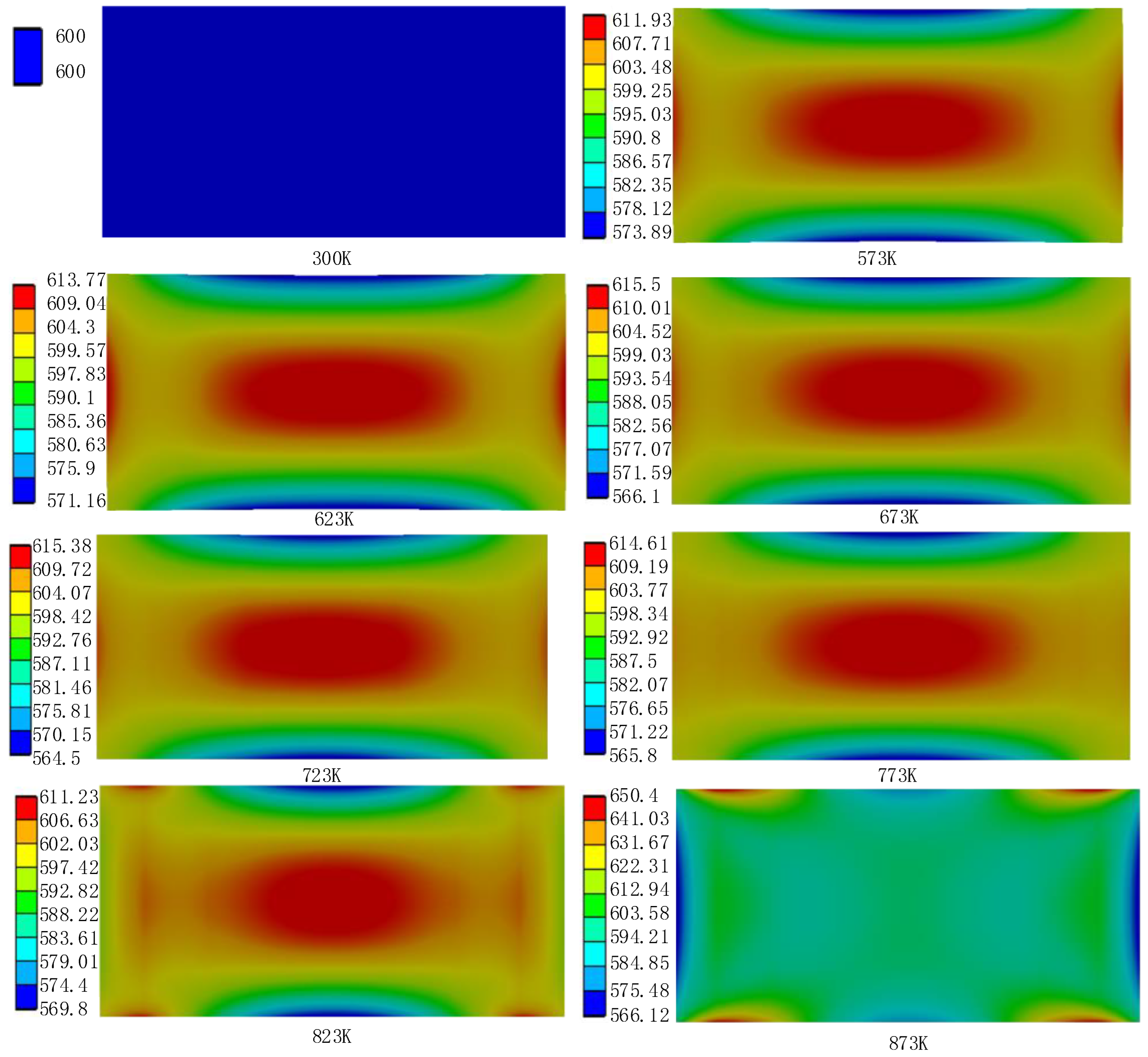
3.4. Temperature–Stress Field Coupling Finite Element Model
4. Microscopic Crack Coefficient Correction
5. Conclusions
Author Contributions
Funding
Institutional Review Board Statement
Informed Consent Statement
Data Availability Statement
Acknowledgments
Conflicts of Interest
References
- Jin, M.; Gao, Y.; Jiang, C.; Gan, J. Defect dynamics in γ-U, Mo, and their alloys. J. Nucl. Mater. 2021, 549, 152893. [Google Scholar] [CrossRef]
- Osetsky, Y.N.; Béland, L.K.; Stoller, R.E. Specific features of defect and mass transport in concentrated fcc alloys. Acta Mater. 2016, 115, 364–371. [Google Scholar] [CrossRef]
- Shi, P.; Xu, W.; Fu, B.; Liu, J.; Zhang, J.; Wang, K.; Liu, X. Pore defects in a nickel-based superalloy with high Ti content. Prog. Nat. Sci. Mater. Int. 2022, 32, 456–462. [Google Scholar] [CrossRef]
- Zhao, S.; Xiong, Y.; Ma, S.; Zhang, J.; Xu, B.; Kai, J.J. Defect accumulation and evolution in refractory multi-principal element alloys. Acta Mater. 2021, 219, 117233. [Google Scholar] [CrossRef]
- Lhadi, S.; Berbenni, S.; Gey, N.; Richeton, T.; Germain, L. Micromechanical modeling of the effect of elastic and plastic anisotropies on the mechanical behavior of β-Ti alloys. Int. J. Plast. 2018, 109, 88–107. [Google Scholar] [CrossRef]
- Essongue, S.; Couégnat, G.; Martin, E. Finite element modelling of traction-free cracks: Benchmarking the augmented finite element method (AFEM). Eng. Fract. Mech. 2021, 253, 107873. [Google Scholar] [CrossRef]
- Chen, J.W.; Zhou, X.P. The enhanced extended finite element method for the propagation of complex branched cracks. Eng. Anal. Bound. Elem. 2019, 104, 46–62. [Google Scholar] [CrossRef]
- Bruhn, T.; Fimland, B.O.; Esser, N.; Vogt, P. STM analysis of defects at the GaAs(001)-c(4 × 4) surface. Surf. Sci. 2013, 617, 162–166. [Google Scholar] [CrossRef]
- Liu, T.; Wu, X.; Sun, B.; Fan, W.; Han, W.; Yi, H. Investigations of defect effect on dynamic compressive failure of 3D circular braided composite tubes with numerical simulation method. Thin-Walled Struct. 2021, 160, 107381. [Google Scholar] [CrossRef]
- Liu, X.; Yuan, L. A cellular automata model for the process of rill erosion. In Proceedings of the International Symposium on Geomatics for Integrated Water Resources Management, Lanzhou, China, 19–21 October 2012. [Google Scholar]
- Chen, Y.; Morishita, K. Molecular dynamics simulation of defect production in Fe due to irradiation. Nucl. Mater. Energy 2022, 30, 101150. [Google Scholar] [CrossRef]
- Tomić, Z.; Gubeljak, N.; Jarak, T.; Polančec, T.; Tonković, Z. Micro- and macromechanical properties of sintered steel with different porosity. Scr. Mater. 2022, 217, 115787. [Google Scholar] [CrossRef]
- Haslberger, P.; Ernst, W.; Schneider, C.; Holly, S.; Schnitzer, R. Influence of inhomogeneity on several length scales on the local mechanical properties in V-alloyed all-weld metal. Weld. World 2018, 62, 1153–1158. [Google Scholar] [CrossRef]
- Xu, A.; Yang, C.; Thorogood, G.; Bhattacharyya, D. Investigating bulk mechanical properties on a micro-scale: Micro-tensile testing of ultrafine grained Ni–SiC composite to determine its fracture mechanism and strain rate sensitivity. J. Alloys Compd. 2020, 817, 152774. [Google Scholar] [CrossRef]
- Chen, X.; Weng, S.; Yue, X.; Fu, T.; Peng, X. Effects of anisotropy and in-plane grain boundary in Cu/Pd multilayered films with cube-on-cube and twinned interface. Nanoscale Res. Lett. 2021, 16, 69. [Google Scholar] [CrossRef] [PubMed]
- Houska, J. Molecular dynamics research of the growth of crystalline ZrO2. Surf. Coat. Technol. 2016, 304, 23–30. [Google Scholar] [CrossRef]
- Parashar, A.; Singh, D. Molecular dynamics based research of an irradiated single crystal of niobium. Comput. Mater. Sci. 2017, 131, 48–54. [Google Scholar] [CrossRef]
- Tang, T.; Kim, S.; Horstemeyer, M.F. Fatigue crack growth in magnesium single crystals under cyclic loading: Molecular dynamics simulation. Comput. Mater. Sci. 2010, 48, 426–439. [Google Scholar] [CrossRef]
- Horstemeyer, M.F.; Farkas, D.; Kim, S.; Tang, T.; Potirniche, G. Nanostructurally small cracks (NSC): A review on atomistic modeling of fatigue. Int. J. Fatigue 2010, 32, 1473–1502. [Google Scholar] [CrossRef]
- Wen, H.; Woo, C.H. Temperature dependence and anisotropy of self- and mono-vacancy diffusion in α-Zr. J. Nucl. Mater. 2012, 420, 362–369. [Google Scholar] [CrossRef]
- Hong, T.W.; Lee, S.I.; Shim, J.H.; Lee, M.G.; Lee, J.; Hwang, B. Artificial Neural Network for Modeling the Tensile Properties of Ferrite-Pearlite Steels: Relative Importance of Alloying Elements and Microstructural Factors. Met. Mater. Int. 2021, 27, 3935–3944. [Google Scholar] [CrossRef]
- Maraveas, C.; Fasoulakis, Z.; Tsavdaridis, K. Mechanical properties of High and Very High Steel at elevated temperatures and after cooling down. Fire Sci. Rev. 2017, 6, 3. [Google Scholar] [CrossRef]
- Qiang, X.; Jiang, X.; Bijlaard, F.; Kolstein, H. Mechanical properties and design recommendations of very high strength steel S960 in fire. Eng. Struct. 2016, 112, 60–70. [Google Scholar] [CrossRef]
- Cantwell, P.; Ma, S.; Bojarski, S.; Rohrer, G.; Harmer, M. Expanding time-temperature-transformation (TTT) diagrams to interfaces: A new approach for grain boundary engineering. Acta Mater. 2016, 106, 78–86. [Google Scholar] [CrossRef]
- Wang, W.; Liu, T.; Liu, J. Experimental study on post-fire mechanical properties of high strength Q460 steel. J. Constr. Steel Res. 2015, 114, 100–109. [Google Scholar] [CrossRef]
- Mirkhalaf, S.M.; Pires, F.A.; Simoes, R. Determination of the size of the Representative Volume Element (RVE) for the simulation of heterogeneous polymers at finite strains. Finite Elem. Anal. Des. 2016, 119, 30–44. [Google Scholar] [CrossRef]
- De Souza Neto, E.A.; Blanco, P.J.; Sánchez, P.J.; Feijóo, R.A. An RVE-based multiscale theory of solids with micro-scale inertia and body force effects. Mech. Mater. 2015, 80, 136–144. [Google Scholar] [CrossRef]
- Cheng, Z.; Wang, H.; Liu, G.R. Fatigue crack propagation in carbon steel using RVE based model. Eng. Fract. Mech. 2021, 258, 108050. [Google Scholar] [CrossRef]
- Xin, R.; Ma, Q.; Li, W. Microstructure and mechanical properties of internal crack healing in a low carbon steel. Mater. Sci. Eng. A 2016, 662, 65–71. [Google Scholar] [CrossRef]
- Akbari, K. The Effect of Prestrain Temperature on Kinetics of Static Recrystallization, Microstructure Evolution, and Mechanical Properties of Low Carbon Steel. J. Mater. Eng. Perform. 2018, 27, 2049–2059. [Google Scholar] [CrossRef]
- Omelyan, I.; Mryglod, I.; Folk, R. Optimized Verlet-like algorithms for molecular dynamics simulations. Phys. Rev. E 2001, 65, 056706. [Google Scholar] [CrossRef]
- Swenson, R.J. Comments on virial theorems for bounded systems. Am. J. Phys. 1983, 51, 940–942. [Google Scholar] [CrossRef]
- Lien, K.H.; Chiou, Y.J.; Wang, R.Z.; Hsiao, P.A. Vector form intrinsic finite element analysis of nonlinear behavior of steel structures exposed to fire. Eng. Struct. 2010, 32, 80–92. [Google Scholar] [CrossRef]
- Hepburn, D.J.; Ackland, G.J. Metallic-covalent interatomic potential for carbon in iron. Phys. Rev. B Condens. Matter 2008, 78, 165115. [Google Scholar] [CrossRef]


| Description | Level | |||||
|---|---|---|---|---|---|---|
| −2 | −1 | 0 | 1 | 2 | ||
| Temperature (/K) | 300 | 500 | 700 | 900 | - | |
| C content (/%) | 1 | 1.3 | 1.6 | 1.9 | 2.2 | |
| Vacancy ratio (/%) | 1 | 2 | 3 | 4 | 5 | |
| Name | Name | ||||||
|---|---|---|---|---|---|---|---|
| 1 | 500 | 1 | 4 | 30 | 900 | 1 | 4 |
| 2 | 900 | 2.2 | 3 | 31 | 900 | 1.6 | 3 |
| 3 | 900 | 1.6 | 2 | 32 | 700 | 1.9 | 5 |
| 4 | 300 | 1 | 3 | 33 | 300 | 1.6 | 4 |
| 5 | 300 | 2.2 | 2 | 34 | 300 | 1 | 5 |
| 6 | 300 | 1 | 1 | 35 | 700 | 1.6 | 4 |
| 7 | 900 | 1.3 | 2 | 36 | 500 | 1.6 | 1 |
| 8 | 300 | 1.9 | 1 | 37 | 500 | 1.3 | 2 |
| 9 | 700 | 1.3 | 2 | 38 | 900 | 1 | 5 |
| 10 | 700 | 1.3 | 5 | 39 | 500 | 1.9 | 1 |
| 11 | 500 | 1.6 | 5 | 40 | 700 | 1.9 | 4 |
| 12 | 700 | 1.6 | 3 | 41 | 300 | 1.3 | 5 |
| 13 | 300 | 1.9 | 3 | 42 | 900 | 1 | 2 |
| 14 | 900 | 1.9 | 5 | 43 | 300 | 1.6 | 2 |
| 15 | 500 | 1 | 3 | 44 | 900 | 1.3 | 1 |
| 16 | 700 | 1.3 | 3 | 45 | 500 | 2.2 | 5 |
| 17 | 300 | 1.9 | 2 | 46 | 300 | 2.2 | 4 |
| 18 | 500 | 1.9 | 4 | 47 | 500 | 1.3 | 3 |
| 19 | 900 | 1.9 | 1 | 48 | 700 | 1 | 4 |
| 20 | 500 | 2.2 | 1 | 49 | 700 | 1.9 | 3 |
| 21 | 700 | 2.2 | 1 | 50 | 500 | 1.6 | 2 |
| 22 | 700 | 1 | 2 | 51 | 900 | 2.2 | 5 |
| 23 | 700 | 2.2 | 2 | 52 | 300 | 2.2 | 3 |
| 24 | 700 | 2.2 | 5 | 53 | 900 | 2.2 | 4 |
| 25 | 300 | 1.3 | 4 | 54 | 500 | 1.3 | 4 |
| 26 | 300 | 1.3 | 1 | 55 | 300 | 1.6 | 5 |
| 27 | 500 | 2.2 | 3 | 56 | 900 | 1.6 | 1 |
| 28 | 700 | 1 | 1 | 57 | 500 | 1.9 | 2 |
| 29 | 700 | 1.6 | 1 | - | - | - | - |
| Name | E/GPa | Q/GPa | Name | E/GPa | Q/GPa | Name | E/GPa | Q/GPa |
|---|---|---|---|---|---|---|---|---|
| 1 | 157 | 10.8642 | 20 | 154 | 11.3220 | 39 | 152 | 11.2760 |
| 2 | 59 | 9.4343 | 21 | 86 | 10.0222 | 40 | 107 | 10.1762 |
| 3 | 46 | 9.5807 | 22 | 89 | 10.0143 | 41 | 211 | 12.2530 |
| 4 | 200 | 12.7287 | 23 | 92 | 10.2568 | 42 | 43 | 9.9332 |
| 5 | 214 | 12.8354 | 24 | 115 | 10.2299 | 43 | 205 | 12.8755 |
| 6 | 192 | 13.2412 | 25 | 208 | 12.4695 | 44 | 35 | 9.8690 |
| 7 | 43 | 9.7222 | 26 | 197 | 13.1815 | 45 | 173 | 10.9962 |
| 8 | 205 | 13.0851 | 27 | 164 | 11.1295 | 46 | 221 | 12.4089 |
| 9 | 90 | 10.0607 | 28 | 83 | 9.9673 | 47 | 155 | 11.0099 |
| 10 | 113 | 10.0334 | 29 | 85 | 10.0065 | 48 | 103 | 10.1257 |
| 11 | 169 | 10.8488 | 30 | 65 | 9.4247 | 49 | 100 | 10.3489 |
| 12 | 98 | 10.3705 | 31 | 56 | 9.4425 | 50 | 154 | 11.1332 |
| 13 | 213 | 12.6229 | 32 | 117 | 10.0845 | 51 | 88 | 9.7228 |
| 14 | 86 | 9.7070 | 33 | 213 | 12.4262 | 52 | 217 | 12.6140 |
| 15 | 153 | 10.9617 | 34 | 206 | 12.2664 | 53 | 72 | 9.4798 |
| 16 | 96 | 10.3152 | 35 | 105 | 10.1922 | 54 | 160 | 10.9185 |
| 17 | 210 | 12.8537 | 36 | 150 | 11.2414 | 55 | 215 | 12.2278 |
| 18 | 167 | 11.0399 | 37 | 151 | 11.1159 | 56 | 36 | 9.7911 |
| 19 | 37 | 9.2974 | 38 | 81 | 9.5083 | 57 | 157 | 11.1803 |
| Sum of Squares | Degrees of Freedom | Mean Variance | F-Value | p-Value | Significance | |
|---|---|---|---|---|---|---|
| 1.94 × 10⁵ | 19 | 10,197.12 | 19,467.81 | <0.0001 | Significant | |
| 16,112.46 | 1 | 16,112.46 | 30,761.08 | <0.0001 | Significant | |
| 35.92 | 1 | 35.92 | 68.58 | <0.0001 | Significant | |
| 265.85 | 1 | 265.85 | 507.54 | <0.0001 | Significant | |
| 132.36 | 1 | 132.36 | 252.69 | <0.0001 | Significant | |
| 914.05 | 1 | 914.05 | 1745.06 | <0.0001 | Significant | |
| 3.66 | 1 | 3.66 | 6.99 | 0.0119 | ||
| 258.85 | 1 | 258.85 | 494.18 | <0.0001 | Significant | |
| 1.75 | 1 | 1.75 | 3.34 | 0.0755 | ||
| 21.88 | 1 | 21.88 | 41.77 | <0.0001 | Significant | |
| 0.2016 | 1 | 0.2016 | 0.3848 | 0.5388 | ||
| 30.15 | 1 | 30.15 | 57.56 | <0.0001 | Significant | |
| 87.22 | 1 | 87.22 | 166.51 | <0.0001 | Significant | |
| 0.013 | 1 | 0.013 | 0.0248 | 0.8757 | ||
| 27.9 | 1 | 27.9 | 53.27 | <0.0001 | Significant | |
| 0.2625 | 1 | 0.2625 | 0.5012 | 0.4834 | ||
| 1.11 | 1 | 1.11 | 2.12 | 0.1538 | ||
| 595.62 | 1 | 595.62 | 1137.13 | <0.0001 | Significant | |
| 0.9142 | 1 | 0.9142 | 1.75 | 0.1946 | ||
| 0.2686 | 1 | 0.2686 | 0.5128 | 0.4784 | ||
| Residual | 19.38 | 37 | 0.5238 | |||
| Total Variation Value | 1.938 × 10⁵ | 56 |
| Sum of Squares | Degrees of Freedom | Mean Variance | F-Value | p-Value | Significance | |
|---|---|---|---|---|---|---|
| 79.88 | 19 | 4.2 | 372.32 | <0.0001 | Significant | |
| 3.32 | 1 | 3.32 | 293.64 | <0.0001 | Significant | |
| 0.0108 | 1 | 0.0108 | 0.9526 | 0.3354 | ||
| 0.0037 | 1 | 0.0037 | 0.327 | 0.5709 | ||
| 0.0111 | 1 | 0.0111 | 0.9809 | 0.3284 | ||
| 0.8068 | 1 | 0.8068 | 71.45 | <0.0001 | Significant | |
| 0.0625 | 1 | 0.0625 | 5.53 | 0.0241 | Significant | |
| 3.51 | 1 | 3.51 | 310.68 | <0.0001 | Significant | |
| 0.0108 | 1 | 0.0108 | 0.9544 | 0.335 | ||
| 0.0135 | 1 | 0.0135 | 1.2 | 0.2807 | ||
| 0.1094 | 1 | 0.1094 | 9.68 | 0.0036 | Significant | |
| 0.259 | 1 | 0.259 | 22.94 | <0.0001 | Significant | |
| 0.1599 | 1 | 0.1599 | 14.16 | 0.0006 | Significant | |
| 0.0079 | 1 | 0.0079 | 0.6966 | 0.4093 | ||
| 0.0006 | 1 | 0.0006 | 0.0519 | 0.8211 | ||
| 0 | 1 | 0 | 0.0032 | 0.9552 | ||
| 0.0003 | 1 | 0.0003 | 0.0229 | 0.8805 | ||
| 0.0725 | 1 | 0.0725 | 6.42 | 0.0156 | Significant | |
| 0.0111 | 1 | 0.0111 | 0.9791 | 0.3288 | ||
| 0.0008 | 1 | 0.0008 | 0.0724 | 0.7894 | ||
| Residual | 0.4178 | 37 | 0.0113 | |||
| Total Variation Value | 80.3 | 56 |
| Model | Standard Deviation | Average Value | Correlation Coefficient R2 | Adjustment Coefficient () | Variation Coefficient (%) | Signal-To-Noise Ratio |
|---|---|---|---|---|---|---|
| 0.7237 | 132.83 | 0.9999 | 0.9998 | 0.5448 | 434.001 | |
| 0.1063 | 10.92 | 0.99448 | 0.9921 | 0.9734 | 59.977 |
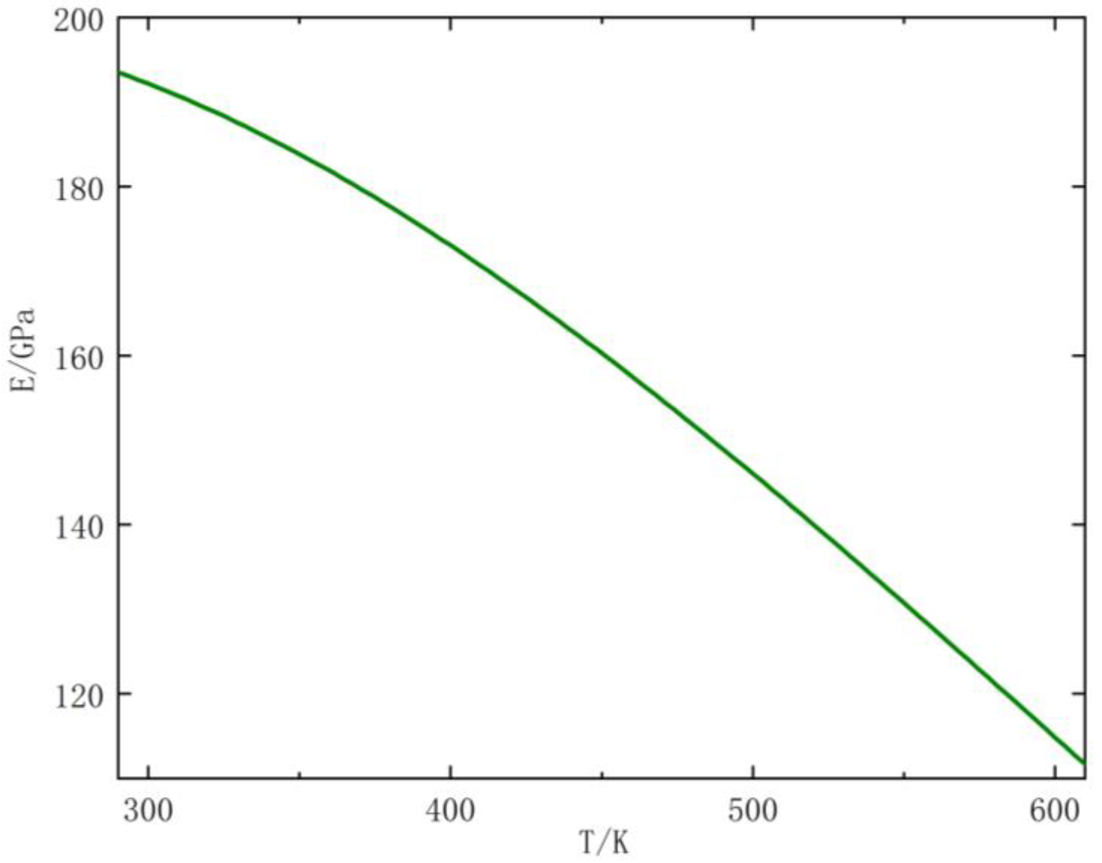
| Temperature (K) | Elastic Modulus (GPa) | Poisson Ratio | Thermal Conductivity (w/mm2) | |
|---|---|---|---|---|
| 300 | 7.8 | 203 | 0.3 | |
| 573 | 7.8 | 195 | — | |
| 673 | 7.7 | 183 | — | — |
| 773 | 7.7 | 169 | — | — |
| 873 | 7.6 | 126 | — | 0.000040 |
| 973 | 7.6 | 35 | — | — |
| Temperature (K) | Maximum Stress (MPa) | Corrected Maximum Stress (MPa) | ||
|---|---|---|---|---|
| 300 | 1593.2 | 1509.8 | 2.655333333 | 2.516333333 |
| 573 | 2055.6 | 1661.9 | 3.578130168 | 2.892826681 |
| 623 | 2515.7 | 1774.2 | 4.100704179 | 2.89202582 |
| 673 | 2610.8 | 1716.1 | 4.600447569 | 3.023911473 |
| 723 | 2807.4 | 1662.1 | 4.946611693 | 2.928604151 |
| 773 | 2909.2 | 1547.4 | 5.13167875 | 2.729533788 |
| 823 | 3022.5 | 1555.4 | 5.304492804 | 2.72972973 |
| 873 | 2982.7 | 1453.1 | 5.110075554 | 2.489506416 |
| Temperature (K) | Maximum Stress (MPa) | Corrected Maximum Stress (MPa) | ||
|---|---|---|---|---|
| 300 | 1734.3 | 1453.6 | 2.8905 | 2.422666667 |
| 573 | 2503.9 | 2091.5 | 4.092342895 | 3.418321484 |
| 623 | 3389.5 | 2084.1 | 5.906389949 | 3.631658738 |
| 673 | 3589.7 | 2110.1 | 5.832832329 | 3.428659636 |
| 723 | 3821.6 | 2043 | 6.211761646 | 3.320763304 |
| 773 | 3975.3 | 1972.7 | 6.4680041 | 3.209677682 |
| 823 | 4047.2 | 1888.8 | 6.621402745 | 3.090162459 |
| 873 | 4024.7 | 1778.7 | 6.698566982 | 2.960404773 |
Disclaimer/Publisher’s Note: The statements, opinions and data contained in all publications are solely those of the individual author(s) and contributor(s) and not of MDPI and/or the editor(s). MDPI and/or the editor(s) disclaim responsibility for any injury to people or property resulting from any ideas, methods, instructions or products referred to in the content. |
© 2023 by the authors. Licensee MDPI, Basel, Switzerland. This article is an open access article distributed under the terms and conditions of the Creative Commons Attribution (CC BY) license (https://creativecommons.org/licenses/by/4.0/).
Share and Cite
Lyu, S.; Gao, Y.; Wang, A.; Hu, Y. Research on Representative Volume Element Fex-Cy High-Temperature Mechanical Model Based on Response Surface Analysis. Appl. Sci. 2023, 13, 11531. https://doi.org/10.3390/app132011531
Lyu S, Gao Y, Wang A, Hu Y. Research on Representative Volume Element Fex-Cy High-Temperature Mechanical Model Based on Response Surface Analysis. Applied Sciences. 2023; 13(20):11531. https://doi.org/10.3390/app132011531
Chicago/Turabian StyleLyu, Shining, Youshan Gao, Aihong Wang, and Yiming Hu. 2023. "Research on Representative Volume Element Fex-Cy High-Temperature Mechanical Model Based on Response Surface Analysis" Applied Sciences 13, no. 20: 11531. https://doi.org/10.3390/app132011531