Battery Charge Control in Solar Photovoltaic Systems Based on Fuzzy Logic and Jellyfish Optimization Algorithm

Abstract

The study focuses on the integration of a fuzzy logic-based Maximum Power Point Tracking (MPPT) system, an optimized proportional Integral-based voltage controller, and the Jellyfish Optimization Algorithm into a solar PV battery setup. This integrated approach aims to enhance energy harvesting efficiency under varying environmental conditions. The study’s innovation lies in effectively addressing challenges posed by diverse environmental factors and loads. The utilization of MATLAB 2022a Simulink for modeling and the Jellyfish Optimization Algorithm for PI-controller tuning further strengthens our findings. Testing scenarios, including constant and variable irradiation, underscore the significant enhancements achieved through the integration of fuzzy MPPT and the Jellyfish Optimization Algorithm with the PI-based voltage controller. These enhancements encompass improved power extraction, optimized voltage regulation, swift settling times, and overall efficiency gains.

1. Introduction

The urgency to mitigate fossil fuel dependency and its environmental repercussions has propelled a global shift towards renewable energy sources (RES) as a viable solution to our energy challenges. The efficiency of renewable energy sources has a significant impact on system management [1]. RES offers a compelling avenue for power generation while concurrently mitigating CO₂ emissions and greenhouse gas effects [2]. Among RES options, solar photovoltaic (PV), hydro, wind, geothermal, and biomass systems are noteworthy [3]. Solar PV is recognized as a leader for future energy needs due to its affordability, simple installation, and minimal maintenance. The maximization of power extraction from PV systems is a critical concern [4]. The inception of Maximum Power Point Tracking (MPPT) in PV systems dates back to 1968 when it was first incorporated into space applications. After this milestone, the widespread adoption of MPPT controllers ensued, significantly enhancing the operational efficiency of PV arrays. Over time, MPPT controllers have evolved to enhance PV array efficiency, adapting to diverse conditions. However, the interplay of irradiance levels, temperature, and other parameters can influence array performance, potentially diminishing conversion efficiency [5]. To address this, researchers have explored diverse MPPT strategies, ranging from traditional linear controllers to innovative approaches like the Jellyfish Search Optimization (JSO) method [6,7]. Despite advances in solar cell technology, challenges persist, including series resistance losses that constrain cell performance. Equivalent circuit derivations are utilized to model and quantify the impact of these internal losses [8,9,10]. Additionally, the integration of thin-film solar cells such as copper indium gallium selenide (CIGS) with wind turbine blades has shown promise in boosting power generation [11]. However, this study contributes significantly by integrating a fuzzy logic-based MPPT system, an optimized PI-based voltage controller, and the Jellyfish Optimization Algorithm into a solar PV battery setup. This innovative integration tackles challenges posed by dynamic environmental factors and loads, ultimately enhancing power extraction efficiency, voltage regulation, and overall performance. The study’s findings further support the use of MATLAB Simulink for modeling and the Jellyfish Optimization Algorithm for PI-controller tuning. The integrated approach’s prowess becomes evident in achieving tangible enhancements through testing scenarios encompassing various irradiation levels. The study’s innovation is characterized by this systematic synergy of methodologies and algorithms, addressing practical challenges and advancing the field of solar energy optimization. Also, this study uses Fuzzy Logic Control (FLC) and the Jellyfish Optimization Algorithm due to their capacity to manage dynamic solar PV system challenges. FLC’s flexibility handles complex environmental interactions, while the Jellyfish Algorithm’s innovative optimization with integrated system uses tuning for improved efficiency and performance. The paper introduces a Fuzzy Logic Controller (FLC) designed for general-purpose embedded processors, specifically applied to the Maximum Power Point Tracking (MPPT) of photovoltaic (PV) energy systems [12]. It utilizes linguistic rules and membership functions, showcasing adaptability to diverse applications, while Jellyfish Optimization, inspired by jellyfish behavior, is specialized for optimization tasks, potentially requiring customization for specific applications [12]. The FLC demonstrates effectiveness by exhibiting consistent results with simulations [12]. The paper explores the use of modified particle swarm optimization (MPSO) with genetic algorithms (GA) to enhance Maximum Power Point Tracking (MPPT) in partially shaded PV systems, outperforming the fuzzy logic controller (FLC) in handling multiple local peaks (LPs). MPSO proves more effective at tracking the global peak (GP), substantially increasing generated power compared to the FLC technique [13].

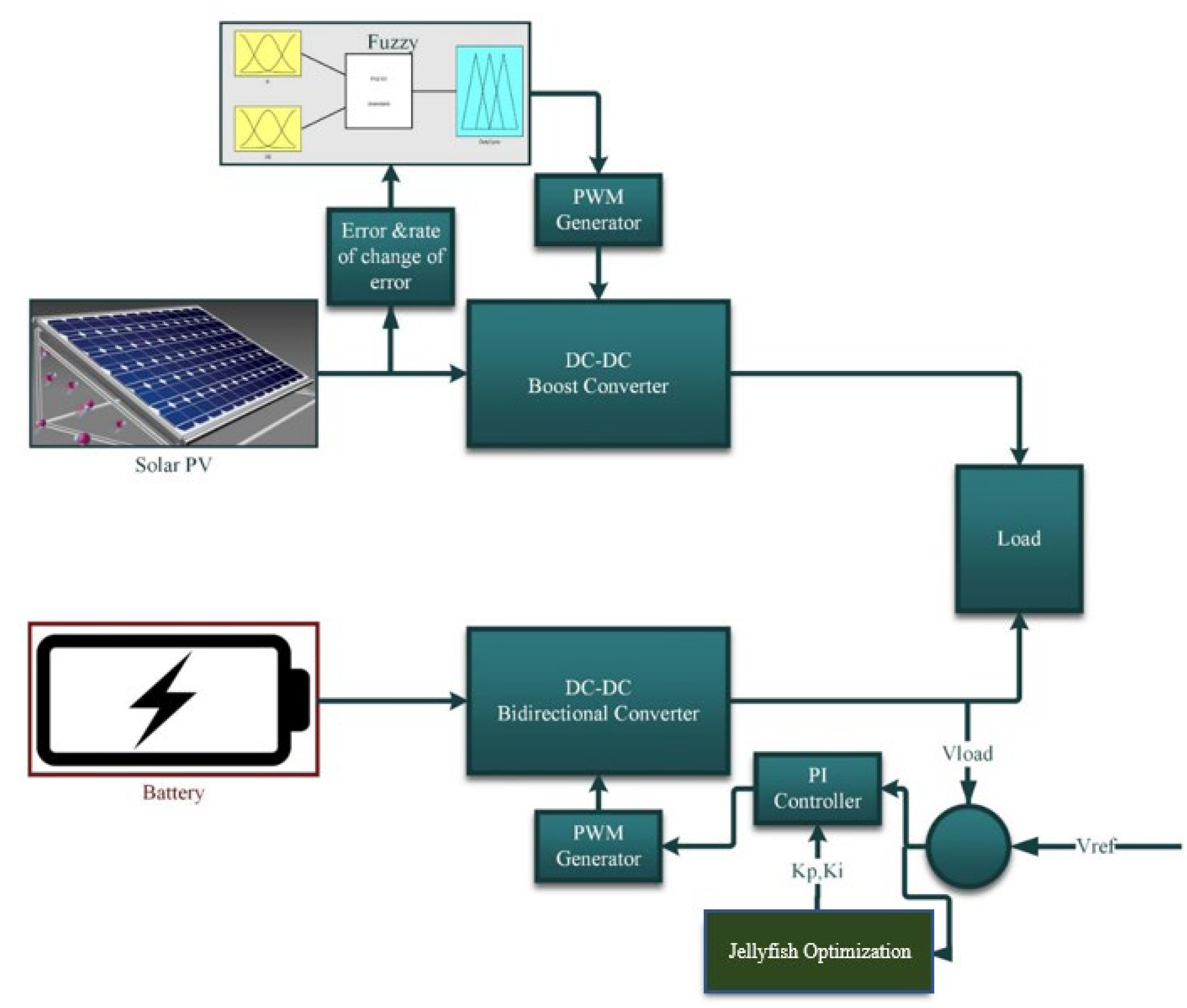
2. Fuzzy and Jellyfish Optimization-Controlled Solar PV Battery System

Figure 1 depicts the Fuzzy and Jellyfish Optimization-Controlled Solar PV system. The following subsections describe the details: a PI controller for a DC–DC bidirectional converter (Jellyfish-Optimized PI controller), a solar PV panel (DC–DC boost converter), a DC–DC bidirectional converter, and a battery.

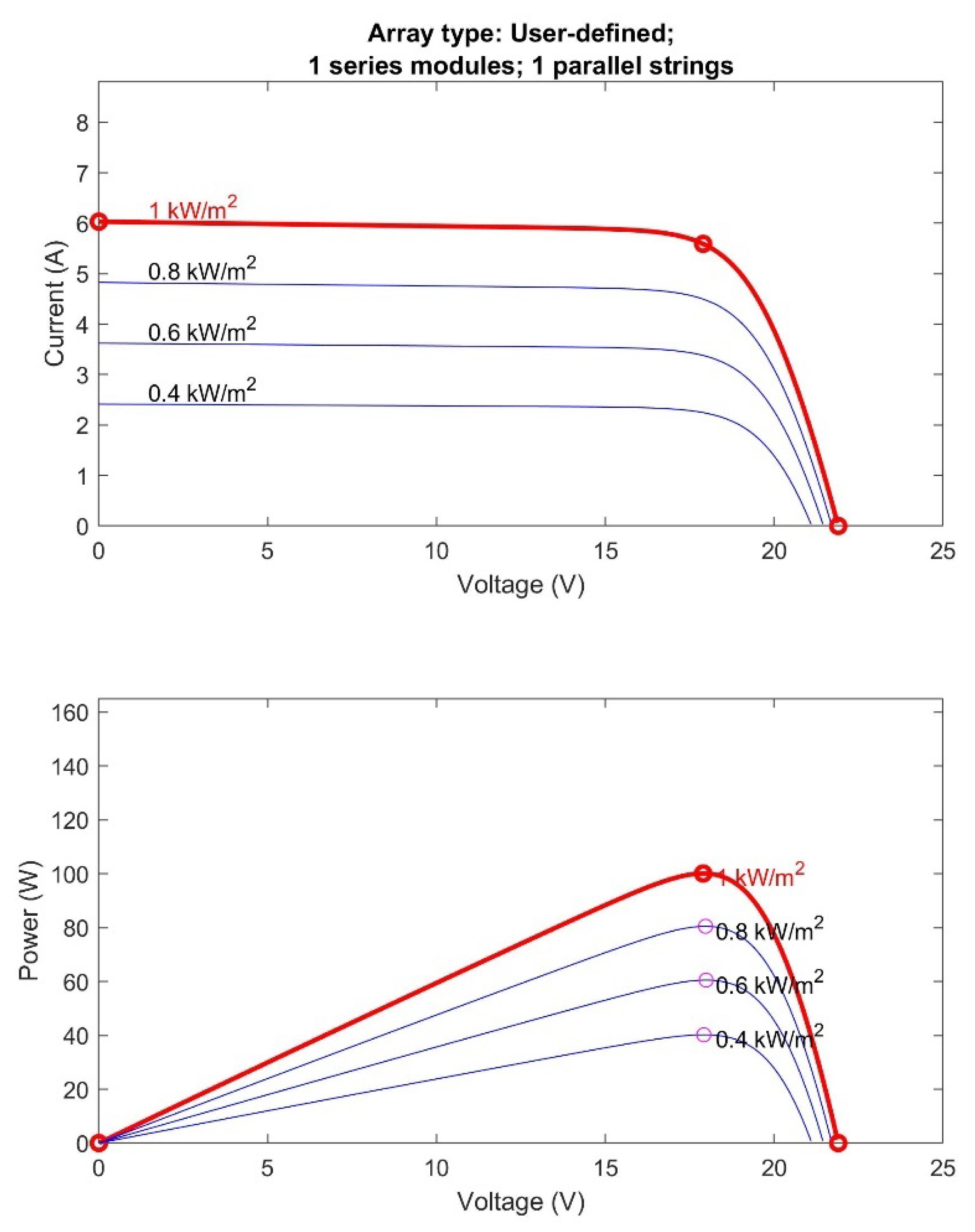
2.1. Solar PV System

Photovoltaic solar cells are semiconductor-based electric devices that convert solar energy into usable electricity. When solar power was paired with a photovoltaic (PV) system, issues arose, such as initial cost, dependability, and generation efficiency. Therefore, simulation and modeling significantly contribute to the investigation, design, and development of PV performance [14].

Due to the low power of photovoltaic solar cells, multiple cells, connected in series or parallel, a PV module connected to the desired current and voltage values, which form a PV array, should be created [15]. Photovoltaic cells have nonlinear properties that vary with temperature and radiation intensity. The PV characteristics curve becomes more complicated when the solar array is partly shaded and more than one peak arises. Because of this, the efficiency of solar cells decreases [16]. There are several reasons why a PV array may become shaded. As an illustration, consider the dust on the panels’ surface and the nearby buildings, trees, and chimneys [17]. Using MPPT algorithms, the optimum efficiency can be achieved for the photovoltaics at different load operating points. The solar module’s power converter’s controller performs MPPT calculations. Figure 2 shows the curves (current–voltage and power–voltage) at the operating position. The use of solar power temperature and irradiation have a nonlinear and unpredictable effect on this property. Typically, two distinct variables must be introduced:

Figure 2 shows the power–voltage and current–voltage characteristics of the PV array under uniform irradiance. The red colored curve shows the maximum power that obtained from the 1000 radiation.

• When the current through the PV cell is 0, open circuit voltage (VOC) is the PV cell voltage.
• When the voltage through the PV cell is 0, short circuit current (ISC) is the PV cell current.

On the I–V curve, a unique point (maximum power point (MPP)) exists where the PV array works at maximum efficiency. The panel’s rating is 100 W, 17.9 V, and 5.59 A.

2.2. DC–DC Boost Converter

In photovoltaic applications, these converters connect the PV module and the output to maximize power extraction. The maximum power point can only be obtained if it is directly connected and operating with the solar panel. Figure 3 depicts the boost converter circuit. It has an output power rating of 150 W at 24 V.

2.3. Fuzzy MPPT Implementation

The fuzzy logic controller determines the optimal duty cycle value. Here, “e” represents the error and “ec” represents the error change/difference in the PV panel’s power slope, so they are the fuzzy inputs. Using a fuzzy logic algorithm, we can calculate the duty cycle.

2.3.1. Fuzzification

Fluffy sets have a set of membership values in the interval [0, 1] generated by the fuzzifier, which is the FLC’s initial component. The error and the change in the error of the power slope deal with triangular membership functions (a particular instance of the trapezoidal function). Seven membership functions represent each input (see Figure 4 and Figure 5), including NB (negative big), NM (negative medium), NS (negative small), and Z (zero).

Fuzzification determines the degree of membership function. It is achieved by determining the degree of membership and then identifying the input in the membership function. From −3 to 3, the membership function’s degree may be described as extreme.

In Figure 4 and Figure 5, the ${\mu }_e$ and ${\mu }_{ce}$ shows the value of the fuzzy for error and changing of error.

Fuzzy input and output are shown in three dimensions in Figure 6.

This figure shows the error and differential error which is shown in X- and Y-axis; the output is the duty cycle value estimated by fuzzy logic, which is shown in Z-axis.

2.3.2. Rule Inference

In the fuzzification step, the level of membership is established. If you have a set of degrees of membership, you need to consider what you should do next. It is ideal to employ fuzzy operators with several antecedents, such as “AND” and “OR”. While evaluating the disjunction of the rule’s antecedents, the fuzzy operator “OR” is used, and when evaluating the rule’s antecedents, “AND” is used. Because the rule’s antecedents must be evaluated in combination, the fuzzy “AND” operator is necessary. The minimal function is utilized because “AND” is the smallest operation between numerous antecedents. Fuzzy logic may also be utilized when several rules produce the same result.

Table 1. Fuzzy final rules.

		E
		NB	NM	NS	Z	PS	PM	PB
ec	NB	Z	Z	Z	NB	NB	NB	NM
	NM	Z	Z	Z	NS	NM	NM	NM
	NS	NS	Z	Z	Z	NS	NS	NS
	Z	NM	NS	Z	Z	Z	PS	PM
	PS	PS	PM	PM	PS	Z	Z	Z
	PM	PM	PM	PM	Z	Z	Z	Z
	PB	PB	PB	PB	Z	Z	Z	Z

lays down the system’s rules of procedure.

The fuzzy roles were chosen based on the performance of the duty cycle response. These roles were manually selected through testing of the outcomes. The duty ratio is used in controlling the PWM switch of the transistor. Fuzzy logic is utilized to ascertain the duty cycle value, where the designation “D” is utilized to represent this value along the Z axis. Figure 7 shows the use of fuzzy logic to determine the duty cycle value.

2.3.3. Defuzzification

The next step is to aggregate the output from each rule into a single value that can be used to adjust the duty cycle. Defuzzification is used to do this. Weighted average defuzzification is employed in the Mamdani approach. The fuzzy output from the rule’s evaluation is multiplied by its singleton value, and the resulting sum is divided by the total sum of all the rule’s fuzzy output. Finally, the single output from this computation may be utilized to adjust the duty cycle.

2.4. Bidirectional DC–DC Converter

A battery energy storage system uses bidirectional DC–DC converters as a battery module–load interface. The voltage control method must be adapted to maintain constant load voltage [18]. Figure 8 depicts a bidirectional DC–DC converter. It has a power rating of 150 W at 24 V.

As shown in Figure 8, U1, D1, Q1, and Cf1 are, respectively, the power input voltage, diode, switch tube, and capacitor for the high-voltage side of the power supply. U2, Q2, D2, and Cf2, respectively, stand in for the power output voltage, switch tube, diode, and capacitor on the low-voltage side of the power supply. The basic one-way buck converter, which is made up of a buck-boost type of bi-directional DC/DC converter circuit to control the state of the two switch tubes and further control the direction of the current and the values of the voltage and current, adds a diode in the position of the switch tube and relocates the switch tube to the original position of the diode [1].

2.5. Voltage Control of DC Bus via Proportional Integral Controller

A comparison is made between the load’s actual and reference voltage. The proportional integral controller is used to handle the erroneous voltage. The PWM generator processes the duty cycle that a proportional integral controller generates. In order to maintain the voltage across the load, a PWM generator controls a bidirectional DC–DC converter. The Jellyfish Optimization Algorithm maximizes the proportional integral controller gains (kp and ki). A detailed explanation of the Jellyfish Optimization Algorithm and PI controller gain adjustment is provided below:

Jellyfish Optimization Algorithm

It is a meta-heuristic algorithm presented in 2021 and is modeled on the swimming behavior of jellyfish. In this algorithm, each problem solution is a jellyfish that looks for food or an optimal solution. Jellyfish or problem solvers have several types of moves to find the optimal solution. Their first movement is based on seawater waves, and their second movement is based on group behavior within groups. The Jellyfish Algorithm, as shown in Figure 9, is modeled from the group behavior of jellyfish and the change of jellyfish with water waves [19]:

This algorithm has types of local and global searches to find the optimal solution, and on the other hand, it has been proven to be more accurate than genetic and PSO algorithms.

A type of swarm intelligence system called the Jellyfish Optimization Algorithm, introduced in 2021, was motivated by jellyfish’s search for food. It is employed to address optimization issues, particularly in engineering and computer science. According to the literature, the Jellyfish method performs better in most real-world applications than several popular meta-heuristic algorithms. A collection of synthetic agents or particles, referred to as “jellyfish”, moves around a three-dimensional space in pursuit of the best answer in the Jellyfish Algorithm. The program is built upon a set of guidelines that mimic the behavior of actual jellyfish. In order to scout the search area and take advantage of interesting solutions, the algorithm employs both random and deterministic movements. The position, speed, and acceleration of the object are some of attributes that are updated based on both its own and the swarm’s most well-known solutions. It can manage many objectives and restrictions. The behavior of sea jellyfish is depicted in Figure 10 together with a model of group motions [20].

The three behaviors of the jellyfish algorithm are as follows:

• A walker or jellyfish can alternate between moving within the group and following the ocean current while intermittently switching the two phases.
• Jellyfish swim throughout the ocean in search of food. They are more attracted to locations with abundant sustenance.
• The quantity of food found depends on the target’s location and function.

The sea’s waves provide nutrients that may draw jellyfish. Equation (1) illustrates how a vector can be used to define the direction of ocean current:

$$\overrightarrow{trend}=\frac{1}{nPop}.\sum {\overrightarrow{trend}}_i=\frac{1}{nPop}\sum \left(X^{*}-e_c{X}_i\right)$$

(1)

Here, $e_c$ represent the absorption factor. Equation (2) can be created by extending Equation (1).

$$\overrightarrow{trend}=X^{*}-\frac{\sum e_c{X}_i}{nPop}=X^{*}-e_c\mu$$

(2)

The best jellyfish, X*, and the average jellyfish population, $\mu$, are used in this calculation. Since $\mathit{d}\mathit{f}={\mathit{e}}_{\mathit{c}}\mu$ can be assumed, this equation can be written in a more general form as Equation (3):

$$\overrightarrow{trend}=X^{*}-\frac{\sum e_c{X}_i}{nPop}=X^{*}-\mathit{d}\mathit{f}$$

(3)

Equations (4) and (5) allow us to consider the distribution of jellyfish at random to be normal.

$$df=\beta \times \mathsf{\sigma }\times ran{d}^f\left(0,1\right)$$

(4)

$$\mathsf{\sigma } =ran{d}^f\left(0,1\right)\times \mu$$

(5)

The jellyfish distribution’s standard deviation index is represented in these relationships by the symbol σ. The usual distribution of jellyfish scattered about the mean point is shown in Figure 11 by the jellyfish.

The displacement process of each jellyfish is shown in Figure 12 both under the influence of the jellyfish community and the water force of the ocean.

Equations (6) and (7) can be used to rewrite equations $\mathit{d}\mathit{f}$ and ${\mathit{e}}_{\mathit{c}}$, respectively:

$$df=\beta \times rand\left(0,1\right)\times \mathsf{\mu }$$

(6)

$$e_c=\beta \times rand\left(0,1\right)$$

(7)

Equation (3) can now be presented in Equation (8) after being rewritten based on Equation (6):

$$\overrightarrow{trend}=X^{*}-\beta \times rand\left(0,1\right)\times \mathsf{\mu }$$

(8)

They are pushed by jellyfish water waves, as shown by Equation (9):

$$X_i \left(t+1\right)=X_i \left(t\right)+rand\left(0,1\right)\times \overrightarrow{trend}$$

(9)

It is possible to expand Equation (9) to Equation (10):

$$X_i \left(t+1\right)=X_i \left(t\right)+rand\left(0,1\right)\times \left(X^{*}-\beta \times rand\left(0,1\right)\times \mu \right)$$

(10)

In this equation, $\mathit{\beta }$ is often equal to three and is a value greater than zero. Jellyfish also move in groups and frequently alternate between two passive and vigorous movements. They look more closely at their surroundings when they are inactive. Equation (11) is used to simulate passive motion:

$$X_i \left(t+1\right)=X_i \left(t\right)+\gamma .rand\left(0,1\right)\times \left(U_b-L_b\right)$$

(11)

In Equation (11), the coefficient of motion is a positive number and typically set at 0.1, is denoted by the symbol $\mathit{\gamma }$. Each dimension’s upper range (${\mathit{U}}_{\mathit{b}}$) and lower range (${\mathit{L}}_{\mathit{b}}$) are indicated by the letter “b”. The jellyfish ${\mathit{X}}_{\mathit{i}}$ randomly chooses the jellyfish ${\mathit{X}}_{\mathit{j}}$ in the active behavior mode, which has two modes. Equation (12) is applied to move if ${\mathit{X}}_{\mathit{i}}$’s merit exceeds ${\mathit{X}}_{\mathit{j}}$’s, and Equation (13) is used in all other cases:

$$X_i \left(t+1\right)=X_i \left(t\right)+rand.\left(X_j \left(t\right)-X_i \left(t\right)\right)$$

(12)

$$X_i \left(t+1\right)=X_i \left(t\right)+rand.\left(X_i \left(t\right)-X_j \left(t\right)\right)$$

(13)

Equation (14) is used to convert between ocean and collective movements:

$$\mathrm{c} \left(t\right)=\left|\left(1-\frac{t}{Maxt}\right)\times \left(2.\mathrm{rand} -1\right)\right|$$

(14)

In this equation, $\mathit{M}\mathit{a}\mathit{x}\mathit{t}$ means the maximum iteration counter and $\mathit{t}$ represents the number of current iterations. Figure 13 displays the $c\left(\mathit{t}\right)$ diagram for the experiment. The jellyfish update is based on group movements if $c\left(\mathit{t}\right)$ is less than 0.5 and on waves if it is larger than 0.5 for each update.

After some iteration and trials, the Jellyfish Optimization sends the gain to the PI controller and receives the integral absolute error as the fitness function. The PI controller uses the JSA results to maintain consistent load voltage. Comparisons are made between the Jellyfish Optimization Algorithm, PSO, and the genetic algorithm.

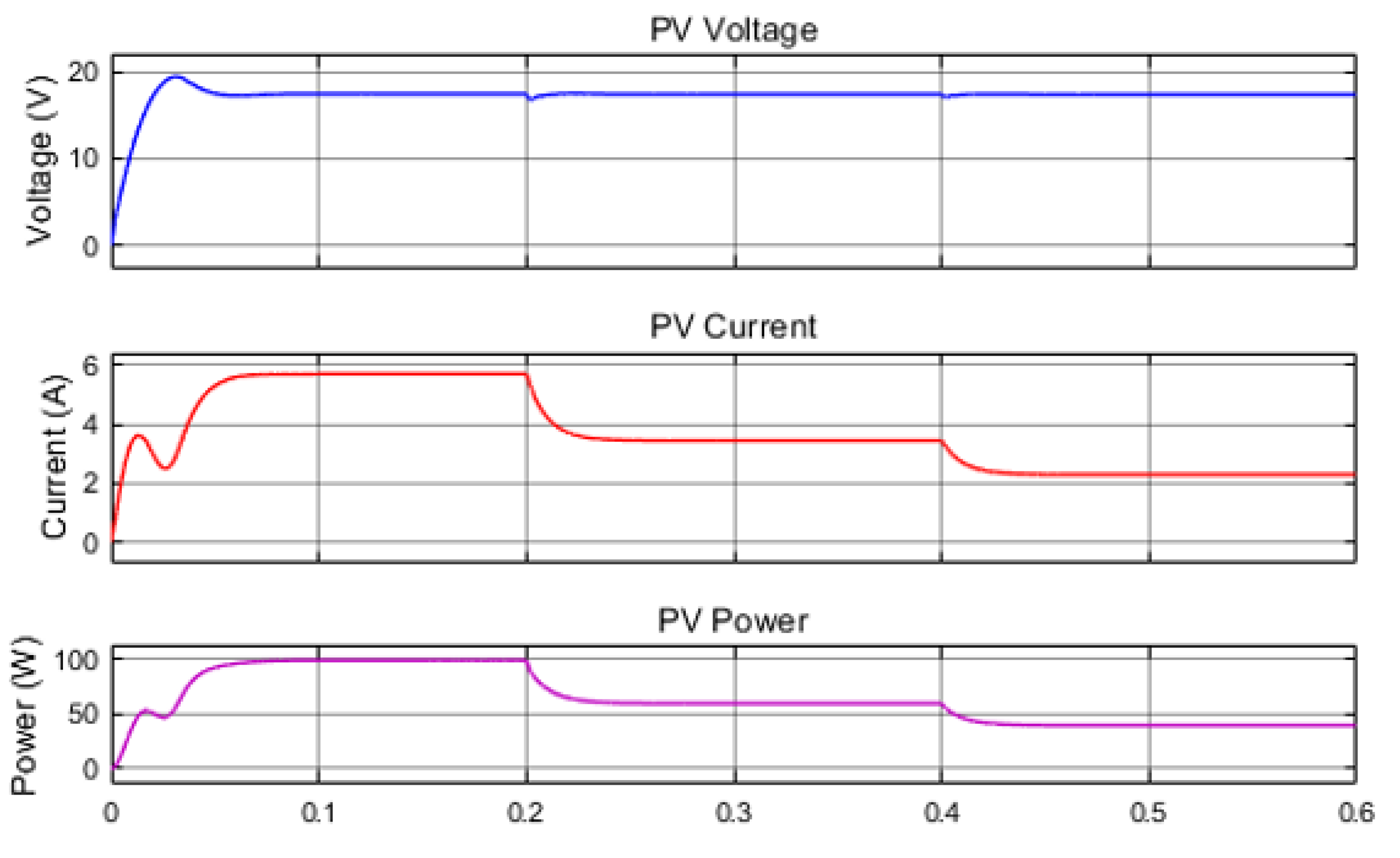
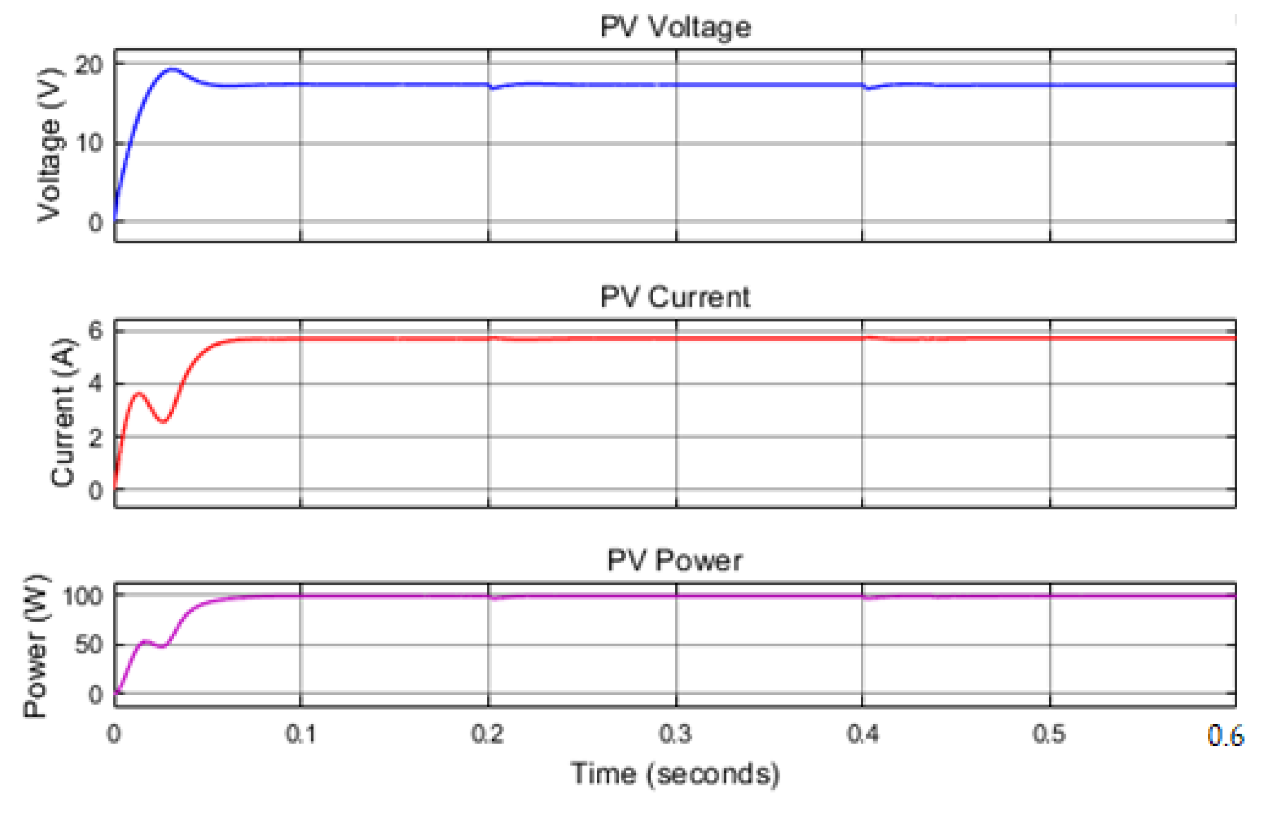
3. Simulation Results and Discussion

The Fuzzy and Jellyfish Optimization-controlled solar PV system was created and simulated in MATLAB. The overall Simulink model of the Fuzzy and Jellyfish Optimization-controlled solar PV battery system is shown in Figure 14.

The gain tuning of the PI controller convergence graph with Jellyfish Optimization, PSO, and GA is shown in Figure 15.

The Jellyfish Optimization Algorithm reaches global fitness value after 17 iterations, but PSO reaches it after 25 iterations and GA after 35 iterations. The value obtained from the Jellyfish Optimization Algorithm is 0.022, but the global point for PSO is 0.025, and for GA, it is 0.035.

Figure 16 shows the solar PV battery system’s load voltage response using Jellyfish Optimization, PSO, and GA.

In Figure 16 the dotted line shows the unit step value. The load voltage response of a GA-optimized PI controller has more overrun and more oscillation. Jellyfish Optimization Algorithm-optimized PI controller has less overrun and faster settling than PSO- and GA-optimized PI controllers. Based on test results, the PI controller optimized by the Hawks Optimization Algorithm provides superior results.

The solar PV battery system was tested for different operating systems, such as constant irradiance, varying irradiance, and varying load conditions. Figure 17, Figure 18 and Figure 19 show the results for constant irradiance conditions (1000 W/m²).

The voltage of the PV panel is 17.4 volts, the PV panel’s power regeneration is 99.5 W, and the PV panel current is 5.71 A. Theoretically, the maximum power is 100 W at 1000 W/m². Still, fuzzy logic MPPT extracts 99.5 W, and the maximum power ratio is 99.5%. The fuzzy logic MPPT extracts the optimum power from a PV panel. The battery voltage, power, and current are 13 Volts, −45.3 W, and −3.48 A, respectively. The battery is in charging mode in this condition. The load current and voltage are 2.08 A and 24 volts, whereas the load power is 50 W. The overall system efficiency is 95.3%. The performance under constant irradiance conditions is shown in

Table 2. Performance of the system under constant irradiance.

Parameter	Voltage (V)	Current (A)	Power (W)
PV	17.4	5.71	99.5
Battery	13	−3.48	−45.3
Load	24	2.08	50

.

Every 0.2 s, the irradiance of the PV panel changes from 1000 to 600 to 400 W/m². Figure 20, Figure 21 and Figure 22 show the results of the system with varying irradiance.

The fuzzy logic MPPT extracts the maximum power PV panel around 99.5 W at 1000 W/m², 59.9 W at 600 W/m², and 39.9 W at 400 W/m². The maximum power ratio is around 98 to 99.5% using fuzzy MPPT. The battery is in charging mode at 1000 and 600 W/m², and the battery is in discharge mode at 400 W/m² to meet the load demand. The system’s overall efficiency improved from 94 to 95.3%. The performance under varying irradiance conditions has been shown in

Table 3. System performance under varying irradiance.

Irradiance	1000 W/m2			600 W/m2			400 W/m2
Parameter	Voltage (V)	Current (A)	Power (W)	Voltage (V)	Current (A)	Power (W)	Voltage (V)	Current (A)	Power (W)
PV	17.4	5.71	99.5	17.4	3.45	59.9	17.4	2.3	39.9
Battery	13	−3.48	−45.3	12.9	−0.549	−7.11	12.9	0.954	12.3
Load	24	2.08	50	24	2.08	50	24	2.08	50

.

The system’s load varied every 0.2 s from 50 to 100 W and then 100 to 150 W. Figure 23, Figure 24 and Figure 25 show the results of the system.

The fuzzy logic MPPT extracts the maximum power PV panel around 99.5 W, and the maximum power ratio is around 99.5% using fuzzy MPPT. The battery charges at 50 W load and discharges when the load is 100–150 W. The overall efficiency of the system is 93.5 to 95.3%. The performance under varying load conditions is shown in

Table 4. System performance under varying load conditions.

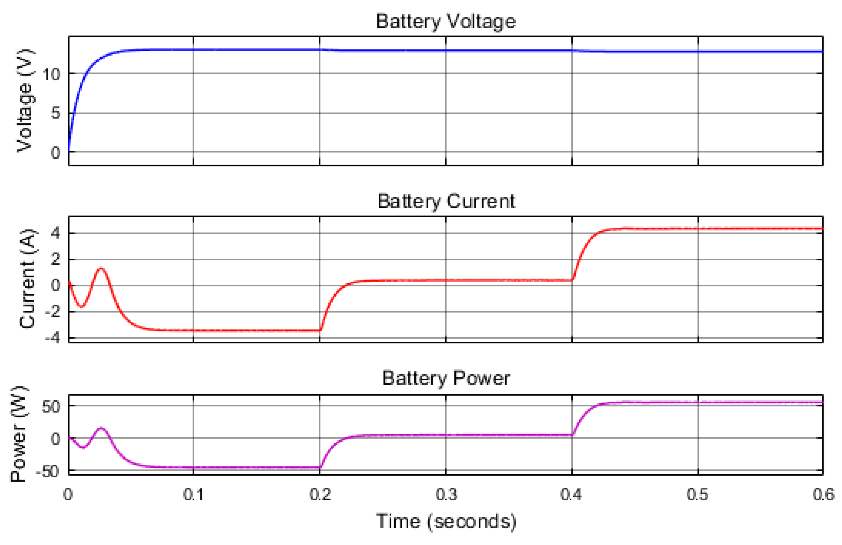
Load	50 W			100 W			150 W
Parameter	Voltage (V)	Current (A)	Power (W)	Voltage (V)	Current (A)	Power (W)	Voltage (V)	Current (A)	Power (W)
PV	17.4	5.71	99.5	17.4	5.71	99.5	17.4	5.71	99.5
Battery	13	−3.48	−45.3	12.9	0.371	4.79	12.8	4.32	55.2
Load	24	2.08	50	24	4.16	100	24	6.25	150

.

The best locations of JSO were 2.8281 and 2.5565 for k_p, and k_i, respectively. Also, the best fitness of JSO was 1.4079. The number of search agents was selected as two (for k_p, and k_i) and the number of the Jelly fish was selected as 30.

In this article, we focused exclusively on normal irradiance conditions, which involve uniform irradiance without factoring in partial shading effects. Under these uniform irradiance conditions, the proposed method demonstrates effective performance.

4. Conclusions

The study employed fuzzy Maximum Power Point Tracking (MPPT) and the Jellyfish Optimization Algorithm to enhance solar photovoltaic (PV) battery systems through a proportional integral voltage controller. The MATLAB-tested system showcased improved proportional integral (PI)-controller values with minimized overshoot and quick settling time. The integration of fuzzy MPPT and the Jellyfish Optimization Algorithm optimized the PI-based voltage controller, effectively extracting maximum power with an extraction ratio of 98–99.5%. The system exhibited an overall efficiency of 93.5–95.3%. Notably, fuzzy MPPT and the Jellyfish Optimization Algorithm successfully optimized the proportional integral-based controller, ensuring constant load voltage while extracting maximum power across diverse operational conditions.

References

- Wazirali, R.; Yaghoubi, E.; Abujazar, M.S.S.; Ahmad, R.; Vakili, A.H. State-of-the-art review on energy and load forecasting in microgrids using artificial neural networks, machine learning, and deep learning techniques. Electr. Power Syst. Res. 2023, 225, 109792. [Google Scholar] [CrossRef]
- Demirbaş, A. Global renewable energy resources. Energy Sources 2006, 28, 779–792. [Google Scholar] [CrossRef]
- Jing, W.; Lai, C.H.; Wong, W.S.H.; Wong, M.L.D. A comprehensive study of battery-supercapacitor hybrid energy storage system for standalone PV power system in rural electrification. Appl. Energy 2018, 224, 340–356. [Google Scholar] [CrossRef]
- Subudhi, B.; Pradhan, R. A comparative study on maximum power point tracking techniques for photovoltaic power systems. IEEE Trans. Sustain. Energy 2012, 4, 89–98. [Google Scholar] [CrossRef]
- Sarvi, M.; Azadian, A. A comprehensive review and classified comparison of MPPT algorithms in PV systems. Energy Syst. 2022, 13, 281–320. [Google Scholar] [CrossRef]
- Alam, A.; Verma, P.; Tariq, M.; Sarwar, A.; Alamri, B.; Zahra, N.; Urooj, S. Jellyfish search optimization algorithm for mpp tracking of pv system. Sustainability 2021, 13, 11736. [Google Scholar] [CrossRef]
- Belhachat, F.; Larbes, C. A review of global maximum power point tracking techniques of photovoltaic system under partial shading conditions. Renew. Sustain. Energy Rev. 2018, 92, 513–553. [Google Scholar] [CrossRef]
- Fong, K.C.; McIntosh, K.R.; Blakers, A.W. Accurate series resistance measurement of solar cells. Prog. Photovolt. Res. Appl. 2013, 21, 490–499. [Google Scholar] [CrossRef]
- Pysch, D.; Mette, A.; Glunz, S.W. A review and comparison of different methods to determine the series resistance of solar cells. Sol. Energy Mater. Sol. Cells 2007, 91, 1698–1706. [Google Scholar] [CrossRef]
- Benghanem, M.S.; Alamri, S.N. Modeling of photovoltaic module and experimental determination of serial resistance. J. Taibah Univ. Sci. 2009, 2, 94–105. [Google Scholar] [CrossRef]
- Gross, R.; Leach, M.; Bauen, A. Progress in renewable energy. Environ. Int. 2003, 29, 105–122. [Google Scholar] [CrossRef] [PubMed]
- Eltamaly, A.M.; Alolah, A.I.; Abdulghany, M.Y. Digital implementation of general purpose fuzzy logic controller for photovoltaic maximum power point tracker. In Proceedings of the SPEEDAM 2010, Pisa, Italy, 14–16 June 2010; pp. 622–627. [Google Scholar]
- Eltamaly, A. Performance of smart maximum power point tracker under partial shading conditions of photovoltaic systems. In Proceedings of the IEEE International Conference on Smart Energy Grid Engineering (SEGE), Oshawa, ON, Canada, 17–19 August 2015; Volume 7. [Google Scholar]
- Crocker, F.A. Prediction of Photovoltaic (PV) Output via Artificial Neural Network (ann) Based on Real Climate Condition. Master’s Thesis, University Tun Hussein Onn, Parit Raja, Malaysia, 2017. [Google Scholar]
- Neupane, S.; Kumar, A. Modeling and Simulation of PV array in Matlab/Simulink for comparison of perturb and observe & incremental conductance algorithms using buck converter. Int. J. Adv. Res. Electr. Electron. Instrum. Eng. 2017, 4, 2479–2486. [Google Scholar]
- Vishwakarma, S. Study of Partial shading effect on Solar Module Using MATLAB. Int. J. Adv. Res. Electr. Electron. Instrum. Eng. 2017, 6, 5303–5308. [Google Scholar]
- Saon, S.; Chee, W.S. Development of optimum controller based on MPPT for photovoltaic system during shading condition. Procedia Eng. 2013, 53, 337–346. [Google Scholar]
- Kotak, V.C.; Tyagi, P. DC to DC Converter in maximum power point tracker. Int. J. Adv. Res. Electr. Electron. Instrum. Eng. 2013, 2, 6115–6125. [Google Scholar]
- Chou, J.-S.; Truong, D.-N. Multiobjective optimization inspired by behavior of jellyfish for solving structural design problems. Chaos Solitons Fractals 2020, 135, 109738. [Google Scholar] [CrossRef]
- Chou, J.-S.; Truong, D.-N. A novel metaheuristic optimizer inspired by behavior of jellyfish in ocean. Appl. Math. Comput. 2021, 389, 125535. [Google Scholar] [CrossRef]