Article

Acceleration of Nuclear Reactor Simulation and Uncertainty Quantification Using Low-Precision Arithmetic

Paul Scherrer Institut, Forschungsstrasse 111, 5232 Villigen, Switzerland
*
Author to whom correspondence should be addressed.
Appl. Sci. 2023, 13(2), 896; https://doi.org/10.3390/app13020896
Submission received: 17 November 2022 / Revised: 27 December 2022 / Accepted: 28 December 2022 / Published: 9 January 2023
(This article belongs to the Special Issue Advanced Computer Architecture)

Abstract

:
In recent years, interest in approximate computing has been increasing significantly in many disciplines in the context of saving energy and computation cost by trading off on the quality of numerical simulation. The hardware acceleration based on the low-precision floating-point arithmetic is anticipated by the upcoming generation of microprocessors and code compilers and has already proven to be beneficial for weather and climate modelling and neural network training. The present work illustrates the application of low-precision arithmetic for the nuclear reactor core uncertainty analysis. We studied the performance of an elementary transient reactor core model for the arbitrary precision of the floating-point multiplication in a direct linear system solver. Using this model, we calculated the reactor core transients initiated by the control rod ejection taking into account the uncertainty of the model input parameters. Then, we evaluated the round-off errors of the model outputs for different precision levels. The comparison of the round-off errors and the model uncertainty showed the model could be run using a 15-bit floating-point number precision with an acceptable degradation of the result’s accuracy. This precision corresponds to a gain of about 6× in the bit complexity of the linear system solution algorithm, which can be actualized in terms of reduced energy costs on low-precision hardware.
Keywords:
RIA; PWR; FPGA; BDF; UQ

1. Introduction

Progress in nuclear power technology heavily depends on the expansion of computing performance. The cutting-edge multiphysics [1,2] and multiscale frameworks [3,4,5], designed to provide more realistic predictions of a reactor core’s safety parameters and to unveil the fundamental mechanisms of nuclear fuel behaviour beyond heuristic correlations, require higher-than-ever computing resources. Over decades, the advance in computing performance has been achieved through transistor miniaturization, which translates into the improvement of the processor design, clock rate speed-up and the high-density multicore architecture. However, nowadays the processor architecture scale is close to its physical limit and it becomes more difficult to shrink [6]. New computing architectures and models will thus be required to continue gaining improvements in chip performance. Optical computing [7], DNA computing [8], coupled oscillating networks [9], approximate computing [10], quantum computing [11] and analogue–digital in-memory computing [12,13] have become important areas of exploration. Another big advance in computing performance is envisioned with the use of traditional computing hardware accelerated for specific engineering tasks. The hardware acceleration of nuclear engineering applications can rely on machine learning methods and approximate computing techniques aimed to trade off the computational quality with speed/energy efficiency.
One of the most promising strategies of approximate computing is the use of a smaller numerical precision in floating-point operations. This idea is motivated by the fact that a high precision of computing hardware is often excessive considering a much lower accuracy is required in practice for engineering applications. Moreover, the solution accuracy is usually limited by physical approximations, numerical errors and the uncertainty of the input data. Therefore, the computing requirement can be decreased in order to redirect the resources into higher spatial, energy or angular resolution or simply to improve the statistics in simulations. This idea has proven to be beneficial for several applications of ocean, weather and climate modelling [14,15] as well as for neural networks training [16]. For a full survey of approximate computing techniques, including their challenges and obstacles, one can read [10].
The usage of a lower precision provides three advantages that can make computation faster. Firstly, a floating-point unit processor requires less work per operation. As an example, switching from double to half precision reduces complexity almost 9 times assuming the best-known Harvey–Hoeven binary multiplication algorithm [17] of complexity O ( n log n ) and 14 times for the Karatsuba algorithm [18] of complexity O ( n 1.585 ) . Secondly, more data can fit in a chip’s cache allowing to speed up memory-bound computations, whose performance depends primarily on the time cost to access memory storing working data. The larger the cache size, the greater number of accesses to the cache that actually find data, hence, the average memory access time becomes less. Empirical studies [19] have shown that the cache miss rate decreases as a power law of the cache size, where the power lies between −0.3 and −0.7, which is equivalent to decreasing by a factor of two if the precision switches from double to half. Thirdly, the lower precision facilitates the communication between parallel processors, whose impairment can seriously slow down computations [20]. Anticipating all these advantages, the low- and multiprecision architectures are now considered as prospective techniques for the acceleration of large-scale applications on the forthcoming high-performance computer systems.
In this paper, we investigated the advantage of low-precision arithmetic for nuclear engineering applications. In nuclear safety analysis, the traditional conservative methods and hypotheses have gradually been replaced with the best estimate plus uncertainty (BEPU) approach [21] meaning that one should produce a series of high-fidelity simulations to quantify the best estimate vector and its uncertainty, for example, by means of the random sampling method. Uncertainty quantification (UQ) is a computationally very expensive part of the BEPU approach as it implies the multiple execution of a high-fidelity code to propagate the uncertainty from the model’s input parameters and the nuclear data to the responses of interest. To address this issue, researchers have developed many acceleration techniques, such as reduced-order modelling [22,23,24], neural networks [25] and automatic differentiation [26] to setup a fast-working heuristic model and bootstrap the best-estimate solution and its variance on the fly. Although reduced order modelling acceleration have achieved a high level of maturity, the simulation of representative samples to train the heuristic model remains quite a time-consuming operation. One can note, however, that there is no much sense in producing high-fidelity simulations with a high accuracy since the uncertainty of engineering parameters likely would exceed the numerical errors by several orders of magnitude. Therefore, the simulations could be performed with a much lower accuracy as long as it did not violate the simulation’s stability and the probability distribution of the responses. This research aims to verify this hypothesis and evaluate the potential speed-up of the UQ for the reactivity-initiated accident in a pressurized water reactor (PWR) core at least for the elementary point-kinetic reactor core model with temperature feedback. Note that this study is focused on the multiprecision analysis of a reactor core simulation rather than on the programming of code on mixed-precision hardware.
The paper is structured as follows. Section 2 discusses the computing hardware that implements the arbitrary-precision arithmetic and the programming software that performs the multiprecision analysis of a computer code. Section 3 shows the results of the multi-precision analysis applied to the uncertainty quantification of a reactor core model. Section 4 contains the conclusions.

2. Multiprecision Hardware

2.1. SIMD

Switching from double to single precision on modern consumer processors does not automatically mean that the computation will be two times faster as the floating-point operation units are designed to perform optimally for 64-bit calculations. However, one can achieve a boost by a vectorization of the algorithm and utilizing SIMD (single instruction, multiple data) or SWAR (SIMD with a register) instructions supported by many modern CPUs and compilers. Notwithstanding SIMD has great savings for cryptography and the processing of 3D graphics, the implementation of a specific algorithm with SIMD is tricky and not automatized.

2.2. Half-Precision

In recent years, lower-precision multiplications accompanied by a higher-precision accumulation have proven useful in training deep neural networks [27]. Traditionally, a neural network has been trained using a single 32-bit precision data type for matrix multiplication and the convolution of vectors. However, it was recognised that half-precision hardware delivers a significant boost of speed while providing similar training quality. That motivated major hardware vendors to settle on mixed-precision hardware units to further enhance their performance [28]. Furthermore, a new floating-point format, BF16, has drawn attention as it is better suited to support deep learning tasks than the standardized FP16 variant due to the right balance between exponent and significant parts of a floating-point number [16]. The comparison of floating-point data types are given in Table A1 of Appendix A.

2.3. FPGA

Notwithstanding the usefulness for neural network applications, the IEEE-754 and BF16 data formats are not necessary the best choices for any other scientific problem. In order to achieve a better optimization of computing resources for arbitrary tasks, a field-programmable gate array (FPGA) has been invented. An FPGA is an integrated circuit which can be configured for a specific functionality and/or data type as it contains an array of transistor logic elements and switchers that can be interwired in various configurations. The circuit is reconfigured using a configuration file developed on a hardware description language such as Verilog, VHDL or OpenCL. The recent Intel C++ and Fortran compilers support programming FPGA devices. Nowadays, FPGA research is an active area of computer science research [14,29] and many hardware vendors invest their efforts into the development of high-efficiency programmable chips.

2.4. Novel Data Types

A software solution is not meant to be efficient for real time execution, as it has to emulate nonstandard numbers and arithmetic on the IEEE-754 floating-point arithmetic units. To address this issue, novel floating-point data types were developed to replace the common floating-point arithmetic on a hardware level. Significance arithmetic relies on the concept of significant digits that carry meaning, contributing to a number, and insignificant digits used for the approximation of numerical errors. Significance arithmetic was extended by [30] to unums and posits which are based on a variable-width storage format for the significand and exponent potentially help to minimize the number of bits used. However, there are several obstacles for the computation in the posit space, including the change of bit length of the number structure and concerns about the numerical stability of algorithms. Another approach is the floating-point adaptive noise reduction (FP-ANR) format suggested by [31]. FP-ANR is compatible with the existing floating-point representation format as it replaces the uninformative bits of the mantissa by a self-detectable pattern. Scanning the mantissa from right to left, one can deduce the number of cancelled bits without using extra memory fields. To conclude, there is a wide range of software solutions emulating the new formats and a short list of implementations on FPGA [32].

2.5. Multiprecision Emulators

The straightforward execution of a piece of code on low-precision hardware likely will produce unacceptable results due to the quality loss or iteration divergence. Therefore, it is useful to experiment with different precision levels to understand the performance of a numerical model prior the porting it onto specialized hardware. To address this goal, a variety of programming tools have been developed to be able to propagate the round-off errors, tune the floating-point numbers’ precision and produce a mixed-precision version of a specific piece of code. One can find a comprehensive review on multiprecision analysis in [33].
A reduced-precision emulator (RPE) [34] provides the capability to emulate calculations in arbitrary reduced floating-point precision. The software program is implemented as a Fortran module that can be included into existing projects. The module defines a new derived type “rpe-var” that emulates a reduced-precision variable and can replace Fortran’s built-in real type in the user’s code. The module provides an overloaded assignment, arithmetic and logic operators that accept “rpe-var” instances as inputs, along with overloaded versions of many of Fortran’s intrinsic functions. The reduction of the precision is applied after each operator or intrinsic function call, while the operations are performed using single-precision arithmetic.

2.6. Multiprecision Analysis Tools

The CADNA (Control of Accuracy and Debugging for Numerical Applications) library [35] estimates the propagation of rounding errors using discrete stochastic arithmetic (DSA). DSA executes each arithmetic operation within user code several times with a randomly chosen rounding error. Then, the statistical analysis of the obtained samples is used to evaluate the number of exact significant digits of the computed result. In addition, the statistical analysis allows one to detect a few types of numerical instabilities during the code execution: nonsignificant operands of multiplication, division or a mathematical function; indeterminism in a branching test; and the sudden loss of accuracy on an addition or a subtraction. The stochastic operations are implemented by overloading the arithmetic operators for stochastic types. The library is designed for C/C++ and Fortran applications

3. Numerical Results

For the numerical illustration, we considered an elementary reactor core model based on the point kinetics equations and the lumped-parameter system of fuel and coolant temperatures; the mathematical formulation of the model is presented in Appendix B. Using this model, we simulated several hot zero power transients initiated by the ejection of control rods worth 1, 1.2, 1.5 and 2 dollars (1$ is equal to one effective delayed neutron fraction). The excessive reactivity was injected gradually over 10 ms and then remained unchanged.
The numerical scheme employed a second-order multistep backward differentiation formula (BDF) method with a variable step size to achieve better performance. The step size selection algorithm benefited Nordsik’s formulation and minimized the local truncation error with respect to the given absolute and relative tolerances. The fixed-point iteration method solved the nonlinear system of equations at every time step. The linear system of equations was resolved by a direct LU decomposition algorithm [36]. The description of the numerical scheme is presented in Appendix C.
The presented reactor core model was analysed as follows
  • Code profiling;
  • Uncertainty propagation;
  • Multiprecision analysis;
  • Multiprecision emulation;
  • Speed-up evaluation.
The first step evaluated the computational time utilized by each part of the code and determined the bottleneck routine; in our example, the most demanding routine was the matrix–vector multiplication performed for the solution of the in-step iteration. The second step propagated the model uncertainty by a random sampling of the input data. The third step propagated the rounding error based on the given uncertainty of the code inputs and evaluated the minimum required precision of every arithmetic operation. The fourth step verified the simulation stability and accuracy; in this step, we evaluated the actual rounding error that must be small compared to the model’s uncertainty. Finally, the fifth step was to compare the performance of the two code versions: (a) the full-precision version that was run on a CPU and (b) the low-precision version programmed on an FPGA. In this work, however, we did not program the low-precision hardware component; instead, we evaluated the potential speed-up in terms of the bit complexity.

3.1. Code Profiling

The model was coded in Fortran and compiled by GCC 8.2.0 using a double precision for all variables. The time spent by each routine was obtained at runtime by the performance analysis tool “GProf” [37]. As was expected, the solution of the in-step linear system ( I h A ) x = b , where h is the time step, by the LU decomposition was the most demanding routine of the code accounting for 95% of the runtime; of that, 85% was devoted to the floating-point operations ×, ÷ and ±, 5% on the cycle loops and 5% on the variable assignment.
The listing of the LU routine is presented in Table 1; the arithmetic complexity was evaluated in percent for a linear system of dimension n = 9 . The algorithm operated over n 2 + n + 2 floating-point variables contained in input matrix A, input vector b, input parameter h and additional parameter S used for the summation. The entries of the matrix and the vector were changed during the algorithm run. At the end of the execution, vector b contained the final result and matrix A consisted of the lower and upper triangular matrices of the input matrix; the diagonal elements of A referred to matrix U, assuming the diagonal entries of L were filled with one.

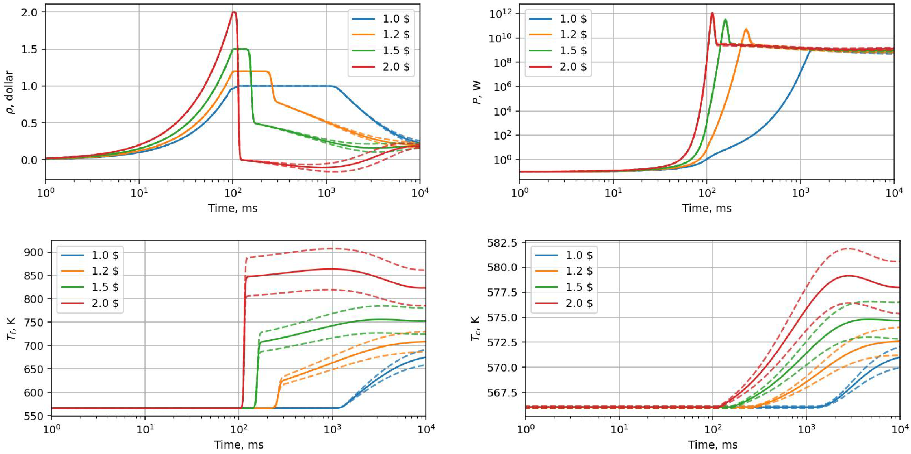
3.2. Uncertainty Propagation

The model uncertainty given in Table A3 of Appendix B was propagated by a run of the 10,000 transients with randomly perturbed inputs. The random samples were generated by the Latin hypercube method using the experimental design package for Python “pyDOE” [38]; this method ensured that the set of randomly generated inputs was a good representative of the real variability of the model input parameters. The variation of the reactor core reactivity ρ , power P, fuel temperature T f and coolant temperature T c for all reactivity perturbations is presented in Figure 1 as a function of time.

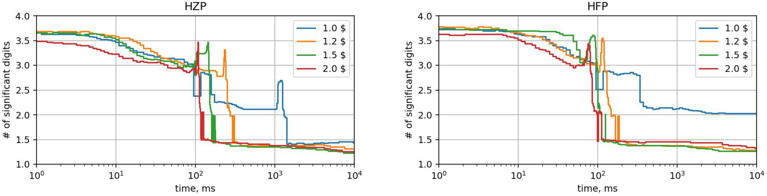
3.3. Multiprecision Analysis

This section presents the multiprecision analysis of the LU algorithm shown in Table 1. The multiprecision analysis aimed to evaluate the minimum precision of A and b entries that was required to propagate the code’s input data without information loss; in general, the larger the uncertainty of the inputs, the smaller the required precision. In order to estimate the exact number of bits and/or digits of the variables of merit, we replaced all the floating-point variables in our code with the stochastic data type provided by CADNA software. The required precision was evaluated for all the variables of the LU algorithm at each time-step iteration.
Figure 2 shows the results of the CADNA analysis applied to matrix A and vector b. At the beginning, matrix I h A defined the system of neutron kinetics and lumped temperature equations coupled by means of the reactor core power; therefore, most entries of the input matrix were equal to zero. The LU algorithm gradually changed the entries of matrix A; however, 21 entries were still kept equal to zero for all iterations due to the input sparse structure. In order to simplify the multiprecision analysis, these entries were excluded from consideration.
The division operation on the lines 9 and 17 of the LU algorithm in Table 1 required special treatment. If the time step h is small, then denominator 1 h x has to preserve a much higher precision than term h x . In order to reduce the complexity of this operation, one should hardcode the function f ( x ) = 1 / ( 1 x ) . Note, this function can be resolved by the Newton–Raphson iterative method with the on-the-fly precision correction algorithm proposed by [39]. In our implementation, we computed the division function using double-precision arithmetic; however, the argument of this function was given in the reduced precision.
Figure 2 shows the precision of A and b varied from two to six decimal digits, which is equivalent to 7 and 20 bits, respectively. The digits referred to the decimal representation of a floating-point number as the binary representation was not available in the CADNA version used. The number of digits varied as a function of time and reactivity as can be seen in Figure 3. One can notice the correlation between the required precision and the time-step history presented in Figure A1 of Appendix B; the smaller the time step used, the higher the precision required. The step size was a function of the local truncation error evaluated by the BDF as the discrepancy between corrector and predictor vectors. The correlation between the required precision and the local truncation error might be useful for a further optimization of the algorithm.

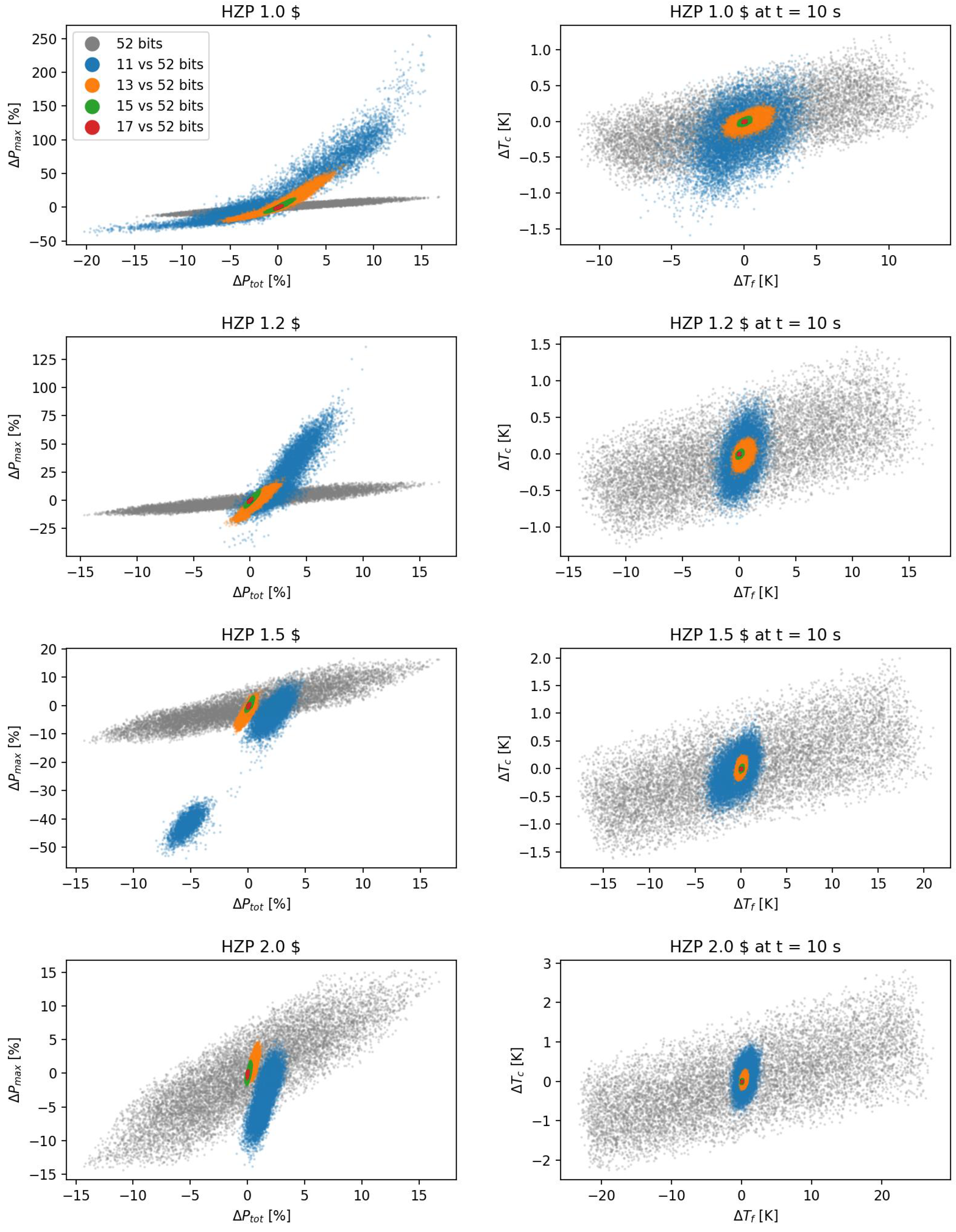
3.4. Multiprecision Emulation

In this section we analyse the stability and accuracy of the low-precision version of the code using RPE [34]. We assumed that the emulator assigned the same number of significant bits for all variables of merit; otherwise, one would have to develop a floating-point arithmetic unit for varied precision, which can be unstable and too complex. The multiprecision analysis provided by CADNA showed that a 17-bit precision arithmetic was required to guarantee that the accuracy of the LU algorithm was enough to propagate the input uncertainty. Firstly, we tested the code for this guaranteed precision; however, the actual precision requirements might have been even lower due to the inaccuracy of the DSA estimation method, and also because the precision estimate varied in time and depended on the index of the matrix entry. Therefore, it was useful to run the code several times while making the precision lower and lower until either the rounding error became too large, or simulation became unstable. In the next paragraph, we show how these criteria were met for the reactor core’s transient model.
The RPE emulation aimed to confirm that the rounding error of the low-precision simulations did not exceed the uncertainty originated from the model’s input. Hence, we calculated and compared two data sets referring to (a) the full-precision simulations produced by the random sampling and (b) the full-to-reduced precision simulation discrepancy produced for the same random samples. Figure 4 shows the full-to-reduced discrepancy in the peaking power P m a x , the total energy release P t o t and the fuel and coolant temperatures at specific time moments. The rounding error computed for the 15-bit precision was comparable to the variation of the parameters of merit due to the uncertainty of the input data. A further drop in precision led to a much higher scope of the rounding errors, and at some point, it resulted in an unstable simulation resulting in a split of the cloud of points.

3.5. Speed-Up Evaluation

In this section, we estimate the potential speed-up of the reduced-precision version of the code in terms of the bit complexity. Figure 4 shows that simulations could be done with an acceptable degradation of the accuracy using 15-bit instead of 52-bit precision for the LU algorithm Table 1. The algorithm performed n 3 3 + n 2 2 5 n 6 multiplications and n ( n + 1 ) 2 divisions, where n = 9 was the rank of matrix A. In our implementation, the reduced-precision code computed the divisions using double-precision arithmetic. Hence, we evaluated the speed-up accounting for the multiplications only, which was about 86% of the floating-point operations. Table A2 shows the gain in the bit complexity of the multiplication function that uses the operands of the reduced precision compared to the double precision. As can be seen, one could reach a 4× to 12× gain in the bit complexity depending on the multiplication algorithm. For example, for the Karatsuba method, the potential speed-up of our algorithm was about six times. Moreover, the use of the reduced precision required four times less inner iterations than that for 52 bits. As a result, the reduced-precision version of the code could potentially be accelerated by about 24 times.

4. Conclusions

The numerical precision of many engineering applications is often excessive in view of the model approximation and input uncertainty. The mixed-precision technique tries to resolve this maladjustment and optimizes the exploitation of the computational infrastructure to make computations faster or more energy efficient. This work presented a brief overview of the existing multiprecision methods, hardware and software; it discussed the status and prospects of half-precision computing, FPGA chips and the novel floating-point number formats. The multiprecision analysis was illustrated for an elementary reactor core model and the uncertainty quantification of the transient initiated by the insertion of reactivity. The analysis performed using RPE and CADNA codes allows us to conclude that there is a large room for the acceleration of nuclear engineering applications on mixed-precision hardware. Future work will be focused on the multiprecision analysis of spatial reactor core models.

Author Contributions

Conceptualization, A.C.; methodology, A.C.; software, A.C.; validation, A.C.; formal analysis, A.C.; investigation, A.C.; resources, A.C.; data curation, A.C.; writing—original draft preparation, A.C.; writing—review and editing, A.C. and A.V.; visualization, A.C.; supervision, A.V.; project administration, H.F.; funding acquisition, A.V. and H.F. All authors have read and agreed to the published version of the manuscript.

Funding

This research was funded by Swiss Nuclear Safety Inspectorate ENSI grant number H-101230.

Institutional Review Board Statement

Not applicable.

Informed Consent Statement

Not applicable.

Data Availability Statement

Not applicable.

Acknowledgments

This work was partly funded by the Swiss Nuclear Safety Inspectorate ENSI (H-101230) and conducted within the framework of the STARS program (http://www.psi.ch/stars, accessed on 2 January 2023).

Conflicts of Interest

The authors declare no conflict of interest.

Sample Availability

Samples of the compounds are available from the authors.

Abbreviations

The following abbreviations are used in this manuscript:
FPGAField-programmable gate array
PWRPressurized water reactor
RIAReactivity initiated accident
UQUncertainty quantification

Appendix A. IEEE-754 Standard

Floating-point numbers represent a finite subset of the continuum of real numbers. Today’s numerical algorithms rely on the conventional single and double IEEE-754 floating-point representation. The IEEE-754 technical standard was introduced by the Institute of Electrical and Electronic Engineering in 1985 to define arithmetic formats, operations on arithmetic formats, rounding rules and exceptions handling. An arithmetic format comprises: (a) finite numbers described by a sign, a fraction and an exponent; (b) positive and negative zeros; (c) positive and negative infinities; (d) quiet and signalling not-a-numbers (NaN). The standard specifies three floating-point basic formats, binary32, binary64 and binary128, and two decimal basic formats, decimal64 and decimal128, which are named for their numeric base and number of bits used for interchange encoding.
As an example, consider how to decode a floating-point number written in the binary32 format. A number
0 0111 0110 0011 0010 1001 1000 0100 001
comprises a sign S (1 bit), an exponent E (8 bits) and a fraction F (23 bits) parts. The sign bit S determines the sign of the number; zero stands for a positive and one for a negative number. The exponent E is stored as an unsigned integer from 0 (all bits are zero) to 255 (all bits are one) and indicates an offset from the actual value by the exponent bias B = 127 . Thus, the exponent ranges from −126 to +127, where 127 represents the actual zero. Values −127 and 128 are reserved for special numbers. The biasing is done to simplify the comparison of two numbers. In our example, the exponent E and fractional F parts read
e = E B = 2 6 + 2 5 + 2 4 + 2 2 + 2 1 127 = 9
f = F / L = 2 3 + 2 4 + 2 7 + 2 9 + 2 12 + 2 13 + 2 18 + 2 23 ,
where L = 2 23 . The true significand includes 23 fraction bits to the right of the binary point and an implicit leading bit to the left of the binary point with value one (unless the exponent is stored with all zeros). Thus, only 23 fraction bits of the significand appear in the memory format, but the total precision is 24 bits. The number in 10-base is written as
a = ( 1 ) s ( 1 + f ) 2 e = 0.0023391323629766703 .
Table A1. Floating-point number size, bits.
BF16FP16FP32FP64
Width16163264
Significand8102352
Exponent75811
Max3.38 × 10 + 38 6.55 × 10 + 4 3.40 × 10 + 38 1.79 × 10 + 308
Min1.17 × 10 38 6.10 × 10 5 1.17 × 10 38 2.22 × 10 308
eps3.06 × 10 03 9.76 × 10 4 1.19 × 10 7 2.22 × 10 16
Table A2. Bit complexity gain of multiplication of two floating-point numbers with n-bit significance compared to the multiplication of two floating-point numbers with 52-bit significance (FP64).
Long MultiplicationKaratsuba [18]Harvey–Hoeven [17]
Precision n O ( n 2 ) O ( n 1.585 ) O ( n log ( n ) )
1122127
131696
151274
17963
19753
21642

Appendix B. Mathematical Model

The model consisted of a point-kinetic approximation of the distribution of neutrons, delayed neutron precursors and a lumped-parameter system of the fuel and coolant temperatures. The model held K groups of precursors represented by the vector λ of decay constants and the vector β of delayed neutron fractions. The equation of the reactor core power P is given by
P t = ρ β l 0 P + λ , C ,
where l 0 is the mean neutron generation time, C is the vector of the precursor’s number density times’ energy release, β = ( 1 , β ) is the total delayed neutron fraction, λ is the vector of delayed neutrons decay constant and ρ is the reactor core reactivity. The last term of the equation represents the delayed neutron source, which is equal to the dot-product of vector λ and vector C .
The equation of the energy release associated with the delayed neutrons is given by
C t = β l 0 P dg λ C ,
where dg λ stands for a diagonal matrix whose main diagonal is vector λ .
Assuming the reactor core comprises fuel and coolant regions, then the time-dependent fuel temperature T f and coolant temperature T c averaged over the corresponding region are described by the lumped-parameter thermal–hydraulic equations. The system of equations for the fuel and coolant temperature change is given by
M f C p f T f t = P + a h ( T c T f ) ,
M c C p c T c t + v T c T i n L = a h ( T f T c ) ,
where M i is a mass, C p i is a specific heat capacity, v is a flow rate, L is the length of the channel, a h is a heat transfer coefficient from the fuel to the coolant regions and T i n is the temperature of the inlet coolant flow.
The reactivity ρ is a function of the coolant and fuel temperatures due to the Doppler and coolant density effects. In this study, we assumed the reactivity was a linear function near a steady-state temperatures of the fuel T f 0 and the coolant T c 0 , that is,
ρ = ρ 0 + α D ( T f T f 0 ) + α c ( T c T c 0 ) ,
where ρ 0 stands for the external reactivity insertion by means of control rods, α D stands for the Doppler reactivity coefficient and α c stands for the total reactivity coefficient of the coolant temperature and density.
The model has two steady-states M 0 and M 1 , which correspond to zero power and to zero reactivity. The former trivial state M 0 given by
M 0 : P = 0 , C = 0 , T f = T i n , T c = T i n ,
remains stable while the total reactivity ρ < 0 . The zero-reactivity state M 1 is given by
M 1 : P = P 0 , C = β l 0 P 0 , T f = T c + P 0 a h , T c = T i n + P 0 M c C p c L v ,
where the steady-state power P 0 is determined by the equation ρ = 0 . In our simulations, the model transient always started from the zero-reactivity state M 1 .
The specific parameters of the model corresponded to a pressurized water reactor (PWR) core. The total fraction β of delayed neutrons was equal to 700 pcm. The lumped parameters of the fuel and coolant thermal–hydraulic model are presented in Table A3. The parameters of the six group emitters are presented in Table A4.
The model simulated the transients initiated by a positive reactivity introduced at the HZP and HFP reactor core states. The excessive reactivity was injected gradually from 0 to 10 ms and then remained unchanged. The reactivity, power, fuel and coolant temperatures responses for all perturbations are presented in Figure 1. The simulation of each case was performed 10 4 times in order to propagate the uncertainty of the input data. A step size on each time iteration was selected automatically to preserve the local truncation error within a given tolerance. The time step and number of internal iteration histories are presented in Figure A1.
Table A3. Parameter values and uncertainties.
ParUnitsValue 3 σ , % Description
P 0 W0.1 10 2 Initial power
l 0 μ s10 10 2 Mean generation time
M f t95 10 2 Fuel mass
M c t15 10 2 Coolant mass
C p f J/kg K2606Fuel heat capacity
C p c J/kg K54006Coolant heat capacity
a f pcm/K−59Doppler coefficient
a c pcm/K19Coolant total temp/dens coefficient
a h MW/K5.49Heat transfer × surface
T i n K566 10 2 Inlet temperature
vm/s5 10 2 Coolant velocity
Table A4. Decay constant λ and fraction β of delay neutron precursors.
N λ , s 1 β , pcm
10.012726.6
20.0317149.1
30.1150131.6
40.3110284.9
51.400089.6
63.870018.2
Figure A1. Time step size (on the left) and number of fixed-point iterations (on the right).
Applsci 13 00896 g0a1

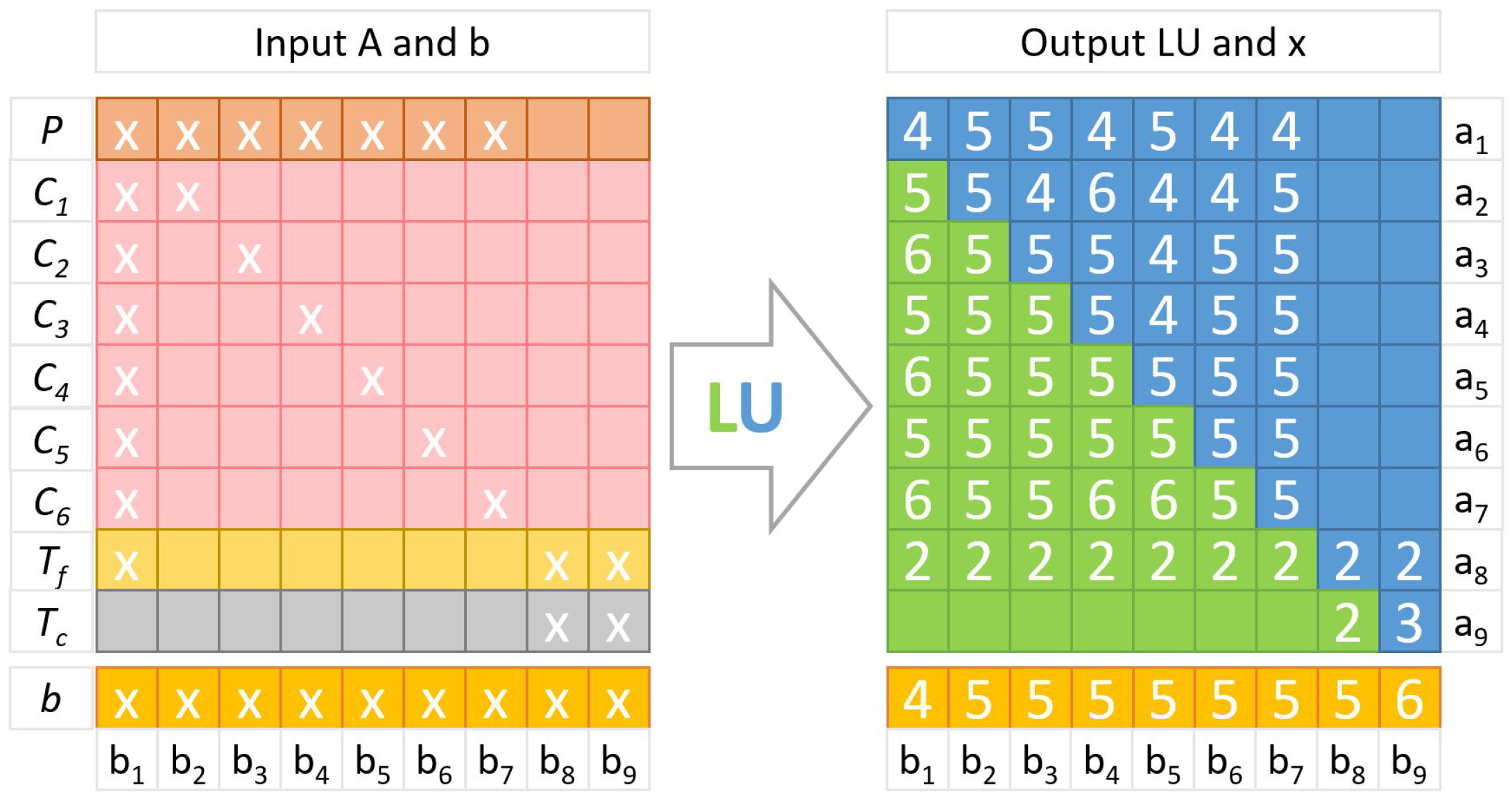
Appendix C. Numerical Scheme

The numerical integration scheme employed the backward differentiation formula (BDF) of the second order with an automatic step-size selection. In order to understand the numerical scheme, consider an ordinary differential equation
x t = f ( t , x ) , for 0 < t < T ,
given initial point x ( 0 ) = x 0 . Let us use Nordsik’s notation and denote z ( t ) the vector of time-derivatives with a step size h > 0 , that is,
z = x , h x ˙ , h 2 2 x ¨ .
The first two components of z 0 are x 0 and f ( 0 , x 0 ) , while the second derivative should be set to zero as we assumed the transient started from a steady state.
Using Nordsik’s notation, the multistep BDF can be formulated as a predictor–corrector scheme. The predictor z h P of Nordsik’s vector at the time point t + h is given by
z h P = 1 1 1 0 1 2 0 0 1 z 0 .
This equation can be extended to an arbitrary order considering the matrix on the right-hand side is the Pascal matrix. The correction step applied to the vector z P is
z h = z h P + l x h x h P .
Here, coefficients l depend on the numerical scheme order. For the second order, l 0 = 0 , l 1 = 3 / 2 and l 2 = 1 / 2 . The solution x ( t + h ) is calculated as follows
x h = x h P + h l 1 1 f ( t + h , x h ) x ˙ h P .
The local truncation error e h of solution x h at the time point t + h relates to the difference between the predictor and corrector vectors z h P and z h . Specifically, for the nth order scheme, the local error is given by
e h = l n x h x h P + O ( h n + 1 ) .
The time step is selected in such a way that the relative local error is less than one. Given absolute and relative tolerances A and R, the step size h is
h = C A + R x h x h x h P 1 n + 1 h ,
where the safety coefficient C = 1.2 .
The extension to the system of ODEs is straightforward. Nordsik’s vector z is replaced by a matrix whose columns correspond to one equation of the ODE system, the division in Equation (A18) is assumed component-wise and the brackets in that equation are replaced by a norm. The other equations of the integration scheme do not change.
The fixed-point algorithm iterates the solution of nonlinear system Equation (A16) to achieve the ultimate convergence for the given floating-point number precision. Specifically, the iteration stops when all the components of solution vector x h become periodical. It is clear that for such a stopping criterion, the higher the floating-point precision used, the more iterations have to be done until convergence. However, the convergence rate of the fixed-point iteration algorithm for the point-kinetic model is rather high; therefore, even for the double precision, the number of iterations is less than 20.

References

  1. Turner, J.A.; Clarno, K.; Sieger, M.; Bartlett, R.; Collins, B.; Pawlowski, R.; Schmidt, R.; Summers, R. The Virtual Environment for Reactor Applications (VERA). Design and architecture. J. Comput. Phys. 2016, 326, 544–568. [Google Scholar] [CrossRef] [Green Version]
  2. Avramova, M.; Abaraca, A.; Hou, J.; Ivanov, K. Innovations in Multi-Physics Methods Development, Validation, and Uncertainty Quantification. J. Nucl. Eng. 2021, 2, 44–56. [Google Scholar] [CrossRef]
  3. Wang, Y.; Schunert, S.; Ortensi, J.; Laboure, V.; DeHart, M.; Prince, Z. Rattlesnake: A MOOSE-Based Multiphysics Multischeme Radiation Transport Application. Nucl. Technol. 2021, 207, 1047–1072. [Google Scholar] [CrossRef]
  4. State-of-the-Art Report on Multi-Scale Modelling of Nuclear Fuels; OECD: Paris, France, 2015.
  5. Cooper, M.W.D. Atomic Scale Simulation of Irradiated Nuclear Fuel. Ph.D. Thesis, Imperial College, London, UK, 2015. [Google Scholar]
  6. Hennessy, J.L.; Patterson, D.A. Computer Architecture: A Quantitative Approach, 6th ed.; Elsevier: Amsterdam, The Netherlands, 2018. [Google Scholar]
  7. Cohen, E.; Dolev, S.; Rosenblit, M. All-optical design for inherently energy-conserving reversible gates and circuits. Nat. Commun. 2016, 7, 11424. [Google Scholar] [CrossRef] [PubMed]
  8. Lewin, D.I. DNA Computing. Nat. Commun. 2002, 4, 5–8. [Google Scholar] [CrossRef]
  9. Wang, T. Novel Computing Paradigms Using Oscillators. Ph.D. Thesis, University of California, Berkeley, CA, USA, 2019. [Google Scholar]
  10. Mittal, S. A Survey of Techniques for Approximate Computing. ACM Comput. Surv. 2015, 48, 1–33. [Google Scholar] [CrossRef] [Green Version]
  11. Weber, L.; Honecker, A.; Normand, B.; Corboz, P.; Mila, F.; Wessel, S. Quantum Monte Carlo simulations in the trimer basis: First-order transitions and thermal critical points in frustrated trilayer magnets. SciPost Phys. 2022, 12, 29. [Google Scholar] [CrossRef]
  12. Xiao, F.; Liang, F.; Wu, B.; Liang, J.; Cheng, S.; Zhang, G. Posit Arithmetic Hardware Implementations with The Minimum Cost Divider and Square Root. Electronics 2020, 9, 1622. [Google Scholar] [CrossRef]
  13. Haq Rashed, M.R.; Jha, S.K.; Ewetz, R. Hybrid Analog-Digital In-Memory Computing. In Proceedings of the 2021 IEEE/ACM International Conference On Computer Aided Design (ICCAD), Munich, Germany, 1–4 November 2021; pp. 1–9. [Google Scholar] [CrossRef]
  14. Jeffress, S.; Duben, P.; Palmer, T. Bitwise Efficiency in Chaotic Models. Proc. R. Soc. A 2017, 473, 20170144. [Google Scholar] [CrossRef]
  15. Russel, F.P.; Duben, P.D.; Niu, X.; Luk, W.; Palmer, T.N. Exploiting the Chaotic Behaviour of Atmospheric Models with Reconfigurable Architectures. Comput. Phys. Commun. 2017, 221, 160–173. [Google Scholar] [CrossRef]
  16. Agrawal, A.; Mueller, S.M.; Fleischer, B.M.; Sun, X.; Wang, N.; Choi, J.; Gopalakrishnan, K. DLFloat: A 16-b Floating Point Format Designed for Deep Learning Training and Inference. In Proceedings of the 2019 IEEE 26th Symposium on Computer Arithmetic (ARITH), Kyoto, Japan, 10–12 June 2019; pp. 92–95. [Google Scholar] [CrossRef]
  17. Harvey, D.; van Der Hoven, J. Integer Multiplication in time O (n log n). Ann. Math. 2021, 193, 563–617. [Google Scholar] [CrossRef]
  18. Karatsuba, A.A. The Complexity of Computations. Proc. Steklov Inst. Math. 1995, 211, 169–183. [Google Scholar]
  19. Hartstein, A.; Srinivasan, V.; Puzak, T.R.; Emma, P.G. Cache miss behavior: Is it 2 . In Proceedings of the 3rd Conference on Computing Frontiers, Ischia, Italy, 3–5 May 2006; pp. 313–330. [Google Scholar]
  20. Liang, L.; Zhang, Q.; Song, P.; Zhang, Z.; Zhao, Q.; Wu, H.; Cao, L. Overlapping Communication and Computation of GPU/CPU Heterogeneous Parallel Spatial Domain Decomposition MOC Method. Ann. Nucl. Energy 2020, 135, 106998. [Google Scholar] [CrossRef]
  21. Best Estimate Safety Analysis for Nuclear Power Plants: Uncertainty Evaluation; Technical Report 52; IAEA: Vienna, Austria, 2008.
  22. Abdel-Khalik, H.S.; Bang, Y.; Kennedy, C.; Hite, J. Reduced Order Modeling for Nonlinear Multi-Component Models. Int. J. Uncertain. Quantif. 2012, 2, 341–361. [Google Scholar] [CrossRef] [Green Version]
  23. Bang, Y.; Abdel-Khalik, H.S.; Hite, J.M. Hybrid Reduced Order Modeling Applied to Nonlinear Models. Int. J. Numer. Methods Eng. 2012, 91, 929–949. [Google Scholar] [CrossRef]
  24. Cherezov, A.; Sanchez, R.; Joo, H.G. A Reduced-Basis Element Method for Pin-by-Pin Reactor Core Calculations in Diffusion and SP3 Approximations. Ann. Nucl. Energy 2018, 116, 195–209. [Google Scholar] [CrossRef]
  25. Phillips, T.R.F.; Heaney, C.E.; Smith, P.N.; Pain, C.C. An autoencoder-based reduced-order model for eigenvalue problems with application to neutron diffusion. Int. J. Numer. Methods Eng. 2021, 122, 3780–3811. [Google Scholar] [CrossRef]
  26. Bokov, P.M.; Botes, D.; Groenewald, S.A. Dual Number Automatic Differentiation as Applied to two-group cross-section uncertainty propagation. Nucl. Technol. Radiat. Prot. 2021, 36, 107–115. [Google Scholar] [CrossRef]
  27. Henry, G.; Tang, P.T.P.; Heinecke, A. Leveraging the bloat16 Artificial Intelligence Datatype for Higher-Precision Computations. arXiv 2019, arXiv:1904.06376. [Google Scholar]
  28. Ho, N.M.; Wong, W.F. Exploiting half precision arithmetic in Nvidia GPUs. In Proceedings of the 2017 IEEE High Performance Extreme Computing Conference (HPEC), Waltham, MA, USA, 12–14 September 2017; pp. 1–7. [Google Scholar] [CrossRef]
  29. Algredo-Badillo, I.; Conde-Mones, J.J.; Hernandez-Gracidas, C.A.; Morin-Castillo, M.M.; Oliveros-Oliveros, J.J.; Feregrino-Uribe, C. An FPGA-based analysis of trade-offs in the Presence of Ill-conditioning and Different Precision Levels in Computations. PLoS ONE 2020, 15, 106998. [Google Scholar] [CrossRef]
  30. Gustafson, J.L. The End of Error: Unum Computing; Chapman and Hall/CRC: Boca Raton, FL, USA, 2015. [Google Scholar]
  31. Defour, D. FP-ANR: A Representation Format to Handle Floating-Point Cancellation at Run-Time. HAL Archive. 2017. Available online: https://hal.inria.fr/lirmm-01549601/ (accessed on 19 December 2022).
  32. Podobas, A.; Matsuoka, S. Hardware Implementation of POSITs and Their Application in FPGAs. In Proceedings of the IEEE International Parallel and Distributed Processing Symposium Workshops, Vancouver, BC, Canada, 21–25 May 2018. [Google Scholar]
  33. Demeure, N. Gestion du Compromis Entre la Performance et la Précision de Code de Calcul. Ph.D. Thesis, Université Paris-Saclay, Paris, France, 2021. [Google Scholar]
  34. Dawson, A.; Duben, P.D. RPE v5: An Emulator for Reduced Floating-Point Precision in Large Numerical Simulations. Geosci. Model Dev. 2017, 10, 2221–2230. [Google Scholar] [CrossRef] [Green Version]
  35. Eberhart, P.; Brajard, J.; Fortin, P.; Jezequel, F. High Performance Numerical Validation using Stochastic Arithmetic. Reliab. Comput. 2015, 21, 35–52. [Google Scholar]
  36. Golub, G.H.; Loan, C.F.V. Matrix Computations, 3rd ed.; Johns Hopkins University Press: Baltimore, MD, USA, 1996. [Google Scholar]
  37. Graham, S.L.; Kessler, P.B.; McKusick, M.K. An execution profiler for modular programs. Softw. Pract. Exper. 1983, 13, 671–685. [Google Scholar] [CrossRef]
  38. pyDOE: The Experimental Design Package for Python. Available online: https://pythonhosted.org/pyDOE (accessed on 19 December 2022).
  39. Chatelain, Y.; Petit, E.; de O. Castro, P.; Lartigue, G.; Defour, D. Automatic Exploration of Reduced Floating-Point Representation in Iterative Methods. In Proceedings of the 25th International Conference Euro-Par 2019 Parallel Processing, Gottingen, Germany, 26–30 August 2019; pp. 481–494. [Google Scholar]
Figure 1. Reactivity, power and temperature transients due to the ejection of a control rod at HZP; the dotted lines show the 3 σ percentile that accounts for 99.7%.
Applsci 13 00896 g001
Figure 2. Number of significant digits estimated by CADNA for 9 × 9 matrix A and vector b and the initial structure of the input matrix; empty cells indicate zero elements.
Applsci 13 00896 g002
Figure 3. Mean number of significant digits over the simulation.
Applsci 13 00896 g003
Figure 4. Reduced-to-full precision discrepancy of power, fuel temperature and coolant temperature.
Applsci 13 00896 g004
Table 1. Arithmetic complexity of the LU algorithm applied to the linear system of equations ( I h A ) x = b of dimension n = 9 .
Arithmetic Complexity
#Code Listing%FLOP
01:do j = 1, n
02:     do i = 1, j
03:          do k = 1, i − 1
04:                 A (i, j) = A (i, j) − A (i, k) ∗ A (k, j)38 n ( n 2 1 ) / 6
05:     do i = j + 1, n
06:           S = A (i, j)
07:          do k = 1, j − 1
08:                 S = S − A (i, k) ∗ A (k, j)26 n ( n 1 ) ( n 2 ) / 6
09:           A (i, j) = S / (A (j, j) − 1/h)10 n ( n 1 ) / 2
10:do i = 1, n
11:     do k = 1, i − 1
12:          b(i) = b(i) − A (i, k) ∗ b(k)10 n ( n 1 ) / 2
13:do i = n, 1, −1
14:      S = −b (i) / h3n
15:     do k = i + 1, n
16:          S = S − A (i, k) ∗ b (k)10 n ( n 1 ) / 2
17:      b (i) = S / (A (i,i) − 1/h)3n
Disclaimer/Publisher’s Note: The statements, opinions and data contained in all publications are solely those of the individual author(s) and contributor(s) and not of MDPI and/or the editor(s). MDPI and/or the editor(s) disclaim responsibility for any injury to people or property resulting from any ideas, methods, instructions or products referred to in the content.

