Development of Fingerprint Identification Based on Device Flow in Industrial Control System

Abstract

With the rapid development of industrial automation technology, a large number of industrial control devices have emerged in cyberspace, but the security of open cyberspace is difficult to guarantee. Attacks on industrial control devices can directly endanger the environment and even life safety. Therefore, how to monitor the industrial control system in real time has become the primary problem, and device identification is the basic guarantee of safety monitoring. There are limitations in building device identification model based on IP address or machine learning. The paper aim at the development of a device traffic fingerprint model and identify the device based on the periodicity of device traffic. The model generates device fingerprints based on pattern sequences abstracted from the traffic and suffix array algorithm. In the process of recognition, the exact pattern matching algorithm is used for preliminary judgment. If the exact pattern matching fails to hit, the final judgment is made by combination fuzzy pattern matching. This paper also proposes a diagonal jump algorithm to optimize the updating of the distance matrix, which saves on the computational cost of fuzzy pattern matching. Simulation results show that compared with SVM, random forest, and LSTM model, the device traffic fingerprint model has good performance advantages in accuracy, recall and precision.

1. Introduction

1.1. Overview

As the main technical support in industrial automation production, industrial informatization has gradually become the basis for automated production in important fields such as national industry, water conservancy, energy and transportation, effectively saving manpower and material resources and improving production efficiency. Because industrial production requires real-time monitoring and operation, industrial control equipment is usually connected to the public Internet, which makes the interaction of information more convenient, but it will also face various security issues in the Internet. Any subtle attack on industrial control equipment can cause significant damage to critical infrastructure, so stronger security mechanisms are needed. In addition, the increasing number of industrial infrastructure security incidents around the world has drawn public attention to the cybersecurity of industrial controls and their unique security needs. Stuxnet, an attack on Iran’s nuclear infrastructure, infected 100,000 computers at 22 production sites and damaged another 1000 centrifuges.

The high economic rewards of attacking industrial systems have led to the rapid development of attack methods, so effective and resilient anomaly detection solutions are needed to deal with evolving attack methods [1]. However, it is difficult for network administrators to manage industrial control systems in terms of security, network resources, and device troubleshooting unless they can identify the devices connected to the industrial control network [2]. From a management and security perspective, device identification can bring multiple benefits to research and industry [3]. Network administrators can inventory devices, look for information leaked due to configuration errors, and determine whether devices are in an abnormal state.

The device identification model is usually constructed based on the extraction of device fingerprints [4,5,6]. The collection methods from fingerprints can be divided into active fingerprints [7] and passive fingerprints [8,9]. Active fingerprinting refers to sending constructed packets to unknown devices, and then constructing device fingerprints according to the response information of the devices. The passive fingerprint is constructed based on the state information of the device in operation without interfering with the normal operation of the device. From the types of fingerprints, it can be divided into physical fingerprints and traffic fingerprints. Physical fingerprints are based on the physical information of the device, such as clock offset, time series composed of register values, etc. The fingerprint built from the device traffic data is the traffic fingerprint. The redundant data packets in industrial control systems can affect normal production processes and even cause network outages. Collecting device physical information requires the deployment of specific monitors, which is expensive and less scalable. The Supervisory Control And Data Acquisition (SCADA) system [10] can easily collect the flow data of the devices in the system. Therefore, this paper will build a device traffic fingerprint library based on passive fingerprints and identify devices.

1.2. Problem Description

The current research work on device fingerprinting is mainly based on machine learning [11,12,13] or neural network [14,15]. However, the device addition and deletion operations are frequent in the industrial control system, and the device view is often changed, and the model trained for a device view will soon become invalid. Even though the model proposed by the literature [16] avoids repeated training, it sacrifices a certain accuracy. Some studies [17,18] build device fingerprints based on traffic characteristics, such as extracting features through special protocol packets such as Domain Name System (DNS) and Address Resolution Protocol (ARP), but many industrial control networks do not have such protocol packets, so corresponding features cannot be extracted. Some systems automatically configure the device network module, so the features extracted from the transport layer and the network layer are almost the same and not unique. Moreover, as the number of devices increases, the accuracy of the feature-based recognition model decreases, and even device confusion occurs. The industrial control system is usually a cyclic production system with a fixed process. The tasks that the equipment is responsible for will not change in a short time, and the data traffic packets sent and received are periodic, so the fingerprint database can be constructed and identified based on the periodicity.

1.3. Author’s Contribution

The process of constructing the device traffic fingerprint recognition model is as follows: first, collect the traffic data of the industrial control device, abstract the data packet into a pattern and obtain the pattern sequence, and then process the pattern sequence through the suffix array algorithm to generate the device fingerprint. When identifying devices, the traffic of unknown devices is abstracted into a query sequence, and then the query sequence is slidably divided into multiple sub-sequences, and then the sub-sequences are matched with all device fingerprints, and the device with the highest matching degree is the identification result. Exact pattern matching is used first, but there is a lot of noise in the industrial control system, and in most cases, exact pattern matching cannot be hit. After exact pattern matching fails, fuzzy pattern matching is used to measure the degree of matching between sequences. In order to improve the scalability of the model, the similarity function is extended from the naive editing distance to the generalized editing distance. In this paper, the diagonal jumping algorithm is also proposed to optimize the generalized editing distance algorithm, which can save the overhead of calculating the distance matrix when the error threshold is small.

1.4. Paper Organization

The rest of this paper is organized as follows: Section 2 briefly reviews the related works of protocol-specific fingerprinting, time-based fingerprinting, and packet feature-based fingerprinting. Section 3 elaborates details of the proposed approaches, while Section 4 gives the experimental results. Conclusions and suggestions on future work are provided in Section 5.

2. Related Work

With the increasing openness of industrial control systems, the attacks are increasing day by day. Once the industrial control system is successfully attacked, it will cause very serious consequences and even cause danger to life [19]. Therefore, it is very important to detect abnormalities and make timely countermeasures. The basis of anomaly detection is device identification. IP address and MAC address are considered to be the ID card of the device, but the address can be tampered with and forged, so relying on the address to identify the device is not reliable. In order to ensure the reliability of device identification, the unique features of the device are extracted and a fingerprint library is constructed. We outline closely related works that fall into three broad categories: protocol-specific fingerprinting, time-based fingerprinting, and packet feature-based fingerprinting.

1. Fingerprints based on specific protocols. Nmap [20] is one of the most well-known active fingerprinting tools, which sends a series of specific requests to identify a device. It can determine the open network ports, running services, and operating system of the device. Nmap also provides a script library based on specific industrial control protocols such as Modbus and EtherNet/IP for collecting service-specific configuration details. GrassMarlin is a passive fingerprint identification tool dedicated to industrial control networks, developed by the National Security Agency (NSA). It provides a database of 54 industrial control protocol fingerprints that identify the types and roles of devices in the network. Keliris et al. [21] construct device fingerprints using the difference between different manufacturers implementing the Modbus protocol. Since each device supporting the Modbus protocol has a set of vendor-specific registers and coil addresses in memory, often containing important details such as the vendor name and firmware version, they read these registers directly through the Modbus protocol to identify industrial control devices. Rodofile [22] et al. propose a range of techniques for DNP3 critical infrastructure reconnaissance. The algorithm can discover DNP3 slaves with their DNP3 addresses and corresponding masters. Li et al. [23] analyze 17 industrial control protocols widely used in industrial control systems and adopt standardized communication to identify industrial control devices. These methods are effective, but rely on specific industrial control protocols, and they are not suitable for other devices that do not support specific protocols.

2. Time-based fingerprinting. Some work focuses on timing analysis of network traffic to identify devices and device types. Literature [6] proposes that using the TCP timestamp option in the TCP header to detect the clock deviation of a single device for single device fingerprinting. In [24], researchers use wavelet analysis to identify wireless access points based on frame arrival interval time increments, but this type of technology is not suitable for an industrial control device, as it relies on access points to route data to fingerprint readers. Radhakrishnan et al. [25] introduce another time-based device fingerprinting technique called “GTID” to identify wireless devices and their types using the distribution of packet arrival intervals. GTID takes advantage of the heterogeneity of different device hardware compositions and variations in device clock skew. Formby [26] et al. propose two methods for device fingerprinting in industrial control networks. The first method identifies industrial control devices by measuring their Cross-Layer Response Time (CLRT), but it only supports industrial control protocols that use “read” and “response” messages. Another physical fingerprinting method identifies industrial control devices by analyzing differences in their operating time. It requires high-resolution operation time, but not all industrial control protocols provide this capability. Oser et al. [27] identify IoT devices by device-specific clock behavior based on immutable IoT hardware settings. Since their classification method is non-intrusive, it may also be suitable for industrial control networks. However, most time-based fingerprinting methods can be affected by buffering in network devices such as switches and routers, which limits their use in real-world environments.

3. Fingerprints based on packet characteristics. Some device fingerprinting studies [11,12,13,28] focus on the characteristics of data packets, and the fingerprinting technology in this paper is similar to these studies. Jeon [24] provides a passive fingerprinting method for industrial control devices based on five characteristics of flow data, namely periodicity, communication persistence, device complexity gap, network service popularity, and segment size. Based on these characteristics, they calculate a ranking score for each device to distinguish between field devices and master servers. However, this approach requires determining the industrial control protocol to be used in advance. IoTSentinel, introduced by Miettinen et al. [28] focuses on identifying device types when they are registered with the network, and IoTSentinel uses the differences in eigenvalues that exist at various layers of packets (e.g., IP, TCP/UDP) to identify specific device types. Shahid et al. [29] propose a machine learning method to identify the type of industrial control devices in the network by analyzing the flow of packets sent and received. The overall accuracy of the random forest classifier is as high as 99.9%. An automatic Internet of Things (IoT) device classification method is described in [30] to identify new and unseen devices. The method extracts features from the perspectives of traffic, packet length, network protocol, and traffic direction to characterize the attributes of various IoT devices. Both methods require a large number of training samples to achieve accurate results.

Based on the collected traffic data, this paper constructs a fingerprint database for all devices in the industrial control system, and identifies the devices through the fingerprint database. The addition or subtraction of devices does not require retraining the model, while ensuring the efficiency and accuracy of recognition.

3. Device Traffic Fingerprint Extraction and Identification

This section will describe the overall process of extracting device traffic fingerprints and identifying location devices based on the fingerprint database. The specific planning is as follows: Section 3.1 describes the process of building a traffic fingerprint library. After the fingerprint library is constructed, Section 3.2 and Section 3.3 introduce how to identify unknown devices based on the fingerprint library. First, the exact matching algorithm in Section 3.2 is used, but the industrial control system has noise, and the exact match often fails to hit. In the case of failure of the exact match, the fuzzy matching algorithm in Section 3.3 is used to further identify the device and give the identification result.

3.1. Device Fingerprint Extraction

The flow data of all devices can be collected from the SCADA system. For a single data packet in the flow data, it is abstracted into a mode $s_i$. The calculation process is as Equation (1):

$$s_i=f(u,l,t,m)$$

(1)

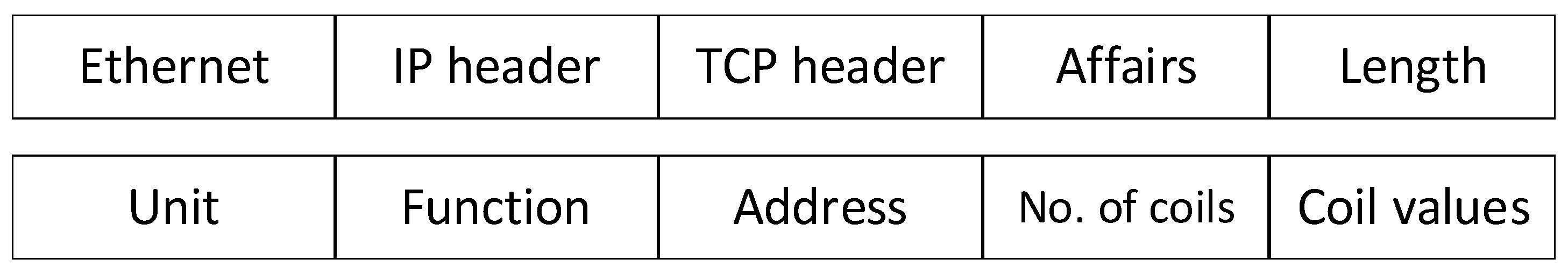
f is an abstract function, the specific implementation depends on the type of industrial control protocol. u represents the specific industrial control protocol, l represents the length of the data packet, t represents the function of the protocol, and m represents the information carried by the protocol. The more information there is, the more patterns are abstracted, resulting in a large difference in the pattern sequence of the same device in different time periods, which cannot be recognized. On the contrary, if the selected information is less, the pattern sequence between different devices will be more similar, causing device confusion. Therefore, characteristic fields with high identification and few changes in the protocol are usually selected. For example, Modbus is a data communication protocol that is based on a request-response model, and is used for transmitting information between devices that are connected to buses or networks over serial lines or Ethernet. The format of Modbus protocol is illustrated in Figure 1. This paper adopts MAC layer, IP layer, TCP layer, transaction, function code, unit, and address information instead of coil value information, because the coil value has a high rate of change and is not suitable for abstraction.

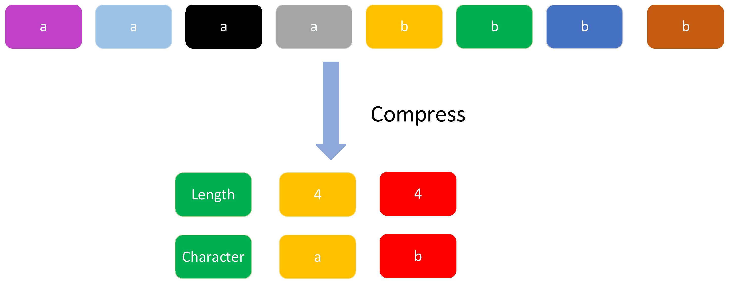
After abstracting the data packet into a pattern, a pattern sequence $Trav=\hspace{0.17em}<s_1,s_2,...,s_n>$ can be obtained. The traffic collected from the industrial control network often has a large number of repeated data packets. If the repeated data packets are not preprocessed, it will not only waste storage space, affect the efficiency of device identification, but also affect the identification accuracy due to the irregular number of repetitions. Therefore, this paper stores the number of repeating patterns and patterns separately, as shown in Figure 2.

The kernel of the industrial control system is a fixed cyclic operation process, and the work that all devices are responsible for will not change easily. Therefore, the collected traffic data has a certain regularity. The pattern sequence can be used as the fingerprint of the device, and then it is identified based on pattern matching. If only the pattern sequence of the device is kept, each match is time-intensive and inefficient. Therefore, this paper uses the suffix matching algorithm to process the pattern sequence. The matching process in the identification only needs $O(k\ast n)$ time complexity, where n is the length of the query sequence, and k is the number of times the query sequence appears in the fingerprint sequence. Suffix matching can be stored in suffix array or suffix tree. Compared with suffix tree, the time overhead of suffix array in matching is almost the same, but it can save storage space. Therefore, this paper adopts the form of suffix array to store.

In order to explain the suffix array generation algorithm more clearly, the concepts used in the algorithm are listed first, as shown in

Table 1. Concepts used by the suffix array generation algorithm.

Subsequence $TraV[i,j]$	A subset of pattern sequences, representing subsequences within any interval of the original sequence. When $1\le i\le j\le n,TraV[i,j]$ is a subsequence.
Suffix	Special subsequence, the subsequence from a certain position to the end of the original sequence, that is, $Suffix[Trav,j]=TraV[j,n]$.
Suffix array SA	Describes a one-dimensional array $SA$ that is sorted in ascending suffix order. $SA\left[i\right]$ represents the starting position of the i-th suffix.
Ranking group RK	Description suffix ranks one-dimensional array $RK$. where $RK\left[i\right]$ is the rank starting with the i suffix.
L/S suffix	If $Suffix[Trav,j]\le Suffix[Trav,j+1]$, then $Suffix[Trav,j]$ is S suffix; if $Suffix[Trav,j]>Suffix[Trav,j+1]$, then $Suffix[Trav,j]$ is L suffix.
L/S model	If $S\left[j\right]\ge S[j+1]$ and $Suffix[Trav,j]\le Suffix[Trav,j+1]$, then $S\left[j\right]$ is S model; If $S\left[j\right]\le S[j+1]$ and $Suffix[Trav,j]>Suffix[Trav,j+1]$, then $S\left[j\right]$ is L model.
S subsequence	The first bit is S model, and d middle models are all L models, which is called Subsequence.
LMS model	If $S\left[i\right]$ is S model and $S[i-1]$ is L model, then $S\left[i\right]$ is LMS model, $Suffix[Trav,i]$ is LMS model.
LMS subsequence	For the LMS subsenquence $TraV[i,j]$, if $i\ne j$, if only $S\left[i\right]$ and $S\left[j\right]$ are LMS models, the rest of the positions are not LMS models. If $i=j$, it can only be the sentinel $ itself.

:

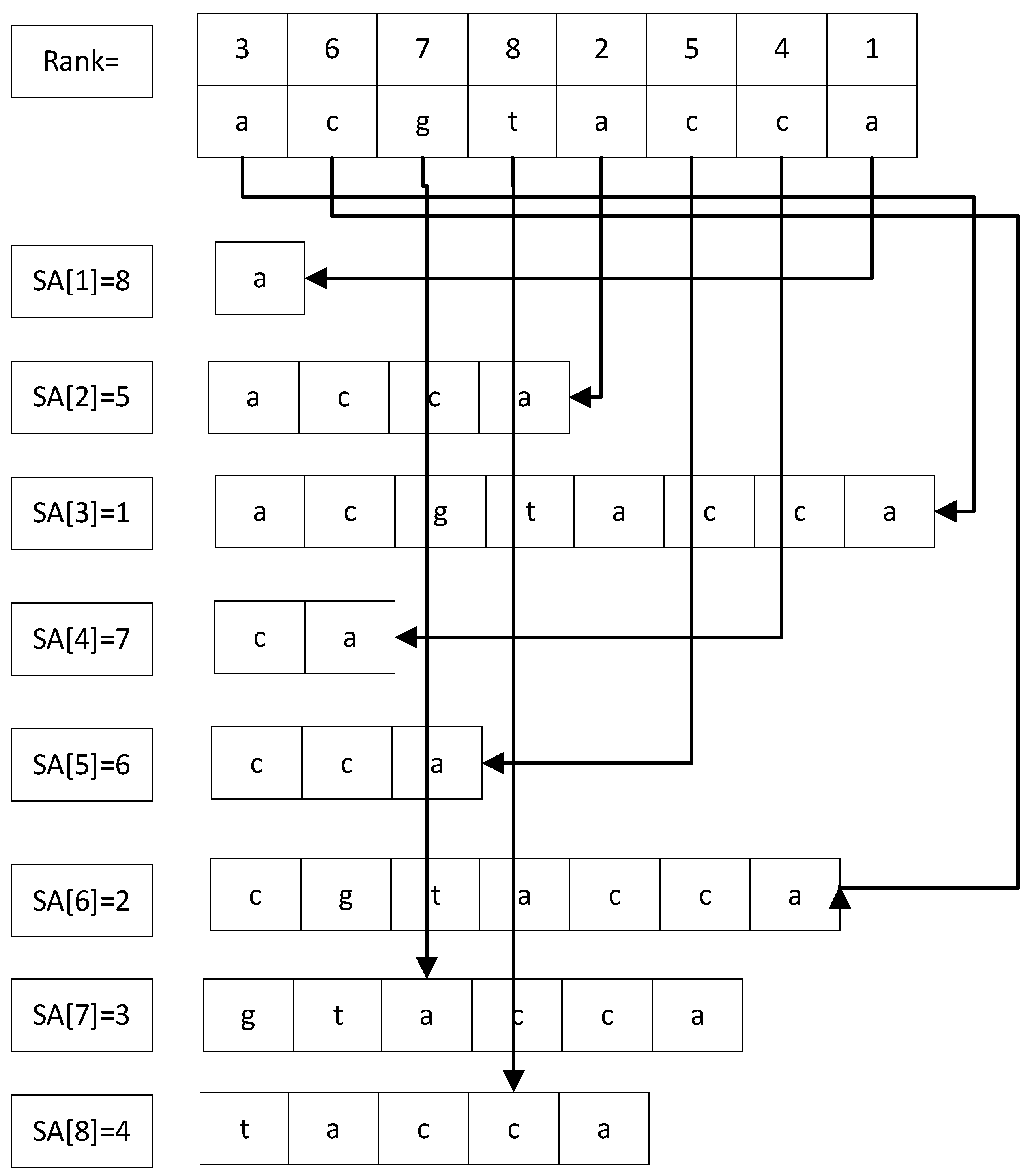
The SA array and the RK array have a reciprocal relationship, that is, $SA\left[RK\right[i\left]\right]=i$, as shown in Figure 3. The time complexity of suffix array-based matching is relatively low, and can be roughly divided into three categories: multiplication algorithm, induced copy algorithm and divide and conquer recursive algorithm. The average time complexity of the multiplication algorithm is $O(n\ast logn)$, but the space overhead is large, and the order of prefixes needs to be stored. The induced copy algorithm first sorts the selected suffixes according to certain rules, and then induces sorting of all suffixes through the sorted suffixes. The disadvantage is that the time complexity of the algorithm is unstable, which is related to the selected suffixes. The divide-and-conquer recursive algorithm first selects a part of the subsequences, arranges them linearly, then renames the shortened pattern sequence to obtain a new pattern sequence, and then recursively arranges the new shortened pattern sequence until the selected subsequences are arranged. Finally, the unselected subsequences are sorted according to the selected subsequences to generate a suffix array. In this paper, the SA-IS algorithm is used to generate the suffix array.

The idea of the SA-IS algorithm [31] is as follows: firstly, mark the L/S suffixes, then sort the LMS subsequences according to the properties of the L/S suffixes, and then induce the sorting of the L suffixes by the LMS subsequences. The S suffix is then induced to sort, and finally the suffix array SA is generated. The overall algorithm flow is shown in Algorithm 1.

Algorithm 1 SA-IS algorithm

Input: Trav: original pattern sequence Output: $SA$: suffix array of pattern sequences 1: Scan Trav from right to left to get the array u, which records the type of each suffix. 2: Scan the array u to get all the LMS subsequences. 3: Induce sorting SA on the LMS subsequence obtained in (2). 4: Rename each LMS subsequence to generate a new pattern sequence. 5: if$Tra{v}_1$ has no repeating moels then 6:     Calculation $S{A}_1$ 7: else 8:     $S{A}_1=SA-IS\left(Tra{v}_1\right)$ 9: end if 10: Use $S{A}_1$ to induce sorting, $SA=induceSA\left(S{A}_1\right)$ 11: return $SA$

First, you need to obtain the sorted LMS suffix. LMS suffixes can be sorted directly using traditional radix sorting, and the time complexity is also $O\left(n\right)$. However, it is difficult to implement radix sorting for pattern sequences, and the constant term in the time complexity is large. The radix sorting will become the performance bottleneck of the entire algorithm. Induced sorting can be used to achieve the sorting of LMS suffixes. The specific process is as follows.

(1) Request an empty pseudo-suffix array $S{A}^{\prime }$ of length n.

(2) Determine the starting position of the S-barrel in each barrel. Put the first pattern of each LMS subsequence into the corresponding bucket according to the sequence in the sequence.

(3) Determine the starting position of the L-barrel in each barrel. Traverse $S{A}^{\prime }$ from front to back. When traversing to $S{A}^{\prime }\left[i\right]$, if $Suffix[Trav,S{A}^{\prime }\left[i\right]-1]$ is L model, then $S{A}^{\prime }\left[i\right]-1$ is put into the L bucket corresponding to the $suffixS{A}^{\prime }\left[i\right]-1$.

(4) Re-determine the starting position of the S-barrel in each barrel. Traverse $S{A}^{\prime }$ from back to front. When traversing to $S{A}^{\prime }\left[i\right]$, if $Suffix[Trav,S{A}^{\prime }\left[i\right]-1]$ is S model, then $S{A}^{\prime }\left[i\right]-1$ is put into the end of S bucket corresponding to the $S{A}^{\prime }\left[i\right]-1$.

(5) It is assumed that the original LMS sequence can be written as $R_1,R_2,...,R_m$ in sequence, where m is the number of LMS subsequences. Assuming w is the number of different LMS subsequences, $V[1,...,m]$ can be renamed for each LMS subsequence. The naming rules are sorted lexicographically from low to high, so that when $R_i<R_j$, $V_i<V_j$, when $R_i=R_j$, $V_i=V_j$, a new pattern sequence $Tra{v}_1=V_1{V}_2{V}_3...V_m$ is generated. The lexicographical relationship of suffixes in $Tra{v}_1$ is the lexicographical relationship of LMS suffixes in $Trav$.

(6) If the same pattern exists in $Tra{v}_1$, the induction operation is performed recursively until there is no same pattern in the newly generated pattern sequence. Swap the name of the LMS subsequence with its current position in $Tra{v}_1$ to generate $S{A}_1$.

After obtaining the suffix array $S{A}_1$ of the LMS subsequence, L suffix and S suffix are induced successively through $S{A}_1$. The specific process is as follows:

(1) Request an empty suffix array $SA$ of length n.

(2) Determine the starting position of the S-barrel in each barrel. The number of L suffixes and S suffixes and the number of each pattern can be obtained when the suffix types are counted in Algorithm 1. According to the characteristics of the suffix array, $S{A}_1$ can directly obtain the sorting of the original LMS suffix. Put all the LMS suffix numbers in the S bucket of the corresponding mode, and the relative order remains unchanged.

(3) Determine the starting position of the L-barrel in each barrel. Traverse SA from front to back. When traversing to $SA\left[i\right]$, if $Suffix[Trav,SA[i]-1]$ is L model, then $SA\left[i\right]-1$ is put into L bucket corresponding to the $suffixSA\left[i\right]-1$.

(4) Re-determine the starting position of the S-barrels in each barrel. SA is traversed from back to front to ensure that each LMS suffix is properly ordered. When traversing to $SA\left[i\right]$, if $Suffix[Trav,SA[i]-1]$ is S model, then $SA\left[i\right]-1$ is put into the end of S bucket corresponding to the $suffixSA\left[i\right]-1]$.

So far, the linear time sorting and the naming calculation $S{A}_1$ are completed first, and then the sorted $S{A}_1$ induces the production of a complete suffix array $SA$, the process of the $SA-IS$ algorithm ends. In the subsequent identification process, a matching operation is required, and the following intermediate variables as shown in

Table 2. Intermediate variables.

f sequence	Sorted sequence of suffixes preceding a pattern
l sequence	A sequence of sorted suffix first patterns
$count$ array	The number of occurrences of each pattern if the f sequence
$position$ array	The starting position of the occurrence of each pattern in the f sequence
$l2f$ array	Map the elements of the l sequence into the f sequence

can be recorded when running the $SA-IS$ algorithm to improve the matching efficiency.

Theorem 1.

When the length of the pattern sequence is n, the time complexity of the $SA-IS$ algorithm is $O\left(n\right)$, and the space complexity is $O\left(n\right|logn\left|\right)$ bits.

Proof. 

Each step of the $SA-IS$ algorithm is computed in linear time. In the worst case, it is necessary to recursively solve the same problem up to half the original size, so the time complexity formula is $T\left(n\right)=T(n/2)+O\left(n\right)$. That is, the $|lo{g}_n|$ layers are recursively calculated, and the problem of each layer is sorted from small to large as $2^0,2^1,2^2,...,2^{|lo{g}_n|}$. The final time complexity is calculated by Equation (2) and the result is $O\left(n\right)$.

$$\sum _{k=0}^{|lo{g}_n|}{2}^k=2\ast 2^{|lo{g}_n|}=O\left(2^{|lo{g}_n|}\right)=O\left(n\right)$$

(2)

The space complexity mainly depends on the space required to store the suffix array to simplify the problem at each recursion. In the first calculation, it consumes at most $O\left(n\right|logn\left|\right)$ bits of storage space, and each recursion will reduce at least half of the storage space. The space complexity is calculated by Equation (3), and the final complexity is $O\left(n\right|logn\left|\right)$. The proof is over.

$$O(\sum _{k=0}^{k_1}n\left|logn\right|/2^k)=O\left((2-1/2^{k_1-1})n\left|logn\right|\right)$$

(3)

The device fingerprint collection process is as follows: first, the device traffic is collected, then abstracted into a pattern sequence, and finally the $SA-IS$ algorithm is used to generate the suffix array and intermediate variables and store them in the device fingerprint database. Then, the location device can be identified using the fingerprint database.    □

3.2. Exact Matching to Identify Unknown Devices

After building the device fingerprint database, the device identification can be completed. After collecting the traffic data of the unknown device, first it is abstracted into an unknown pattern sequence Trav according to the Formula (1), and then it is slidably divided into multiple subsequences $Trav[i,j]$. The subsequences are matched with all fingerprint sequences in the fingerprint database, and the device with the highest matching degree is the identification result. The first step of matching is exact matching, that is, the subsequence is required to be a successful match only if it completely matches the device fingerprint sequence. The exact matching base adopts the FM index sequence matching algorithm, and the overall algorithm flow is shown in Algorithm 2.

Algorithm 2 FM index matching algorithm

Input:$f[1:n]:$ Sorted suffix first pattern sequence. $l[1:n]:$ Sorted fuffix preceding pattern series. $position[1:n]:$ The starting position of the pattern in the f sequence. $pattern:$ pattern sequence to be queried. $count[1:n]:$ The number of occurrences of the pattern in the f sequence. $l2f:$ The correspondence between the f sequence and the l sequence elements. Output: $match[1,m]:$ Record the position where the query pattern sequence appears in the original pattern sequence. 1: Calculate the position $p_f$ where the character c at the end of the pattern sequence appears in the sequence f using the count array and the position array. 2: Determine whether the element at the position of $p_f$ in the l sequence is equal to the previous element of c, If it is not equal, it will be discarded, and if it is equal, it will be recorded in $p_l$. 3: Reverse mapping $p_l$ to the f sequence via l2f produces a new position array $p_f$, and updates c to its previous character. 4: Execute step (2), if the number of elements of $p_l$ is 0, it means that there is no strict match, and the calculation is terminated. 5: When the pattern sequence traversal is completed, the final sequence $p_f$ is obtained. 6: Map $p_f$ to the position array match where the pattern sequence appears in the original pattern sequence through the suffix array $SA$.

For the original pattern sequence $Trav=ACCGATG$, the query sequence pattern = GA. The matching process is shown in Figure 4.

After obtaining the position match of the query sequence pattern in the original pattern sequence $Trav$, the matching score with the fingerprint sequence will be calculated by Equation (4), and the fingerprint sequence with the highest matching score will be determined as the final recognition result.

$$sc=\sum _1^n(\sum _1^m\sum _i^j{len}_{pattern}/{len}_{Trav}\ast {totallen}_{pattern})/{totallen}_{Trav}$$

(4)

${totalLen}_{Trav}$ represents the total length of the fingerprint sequence. ${len}_{pattern}$ indicated the number of consecutive repetitions of each matching pattern in the query subsequence. ${len}_{Trav}$ indicates the number of repetitions of the matching pattern in the fingerprint sequence. ${totalLen}_{pattern}$ indicates the length of each subsequence of the query sequence. Finally, the evaluation scores of all subsequences are accumulated to caluculate the evaluation score of the query sequence.

Match the query sequence with the fingerprints in the fingerprint database one by one, and the device with the highest matching score is the final identification result. However, relying only on exact matching is not ideal in many cases, because there is a lot of noise in the industrial control system, filled with a large number of redundant data packets with an indeterminate number, and the content or type of data packets in different periods are not the same. Periods are not stable. The conditions for exact matching are strict, and all fingerprint matching scores may be 0, resulting in the device not being recognized. In order to solve the problem, this chapter adopts fuzzy matching to identify the device in the case that exact matching cannot be identified.

3.3. Fuzzy Matching to Identify Unknown Devices

Because the exact matching conditions are strict, the query sequence may not match any device fingerprint, so fuzzy pattern matching will be used for the final device identification. 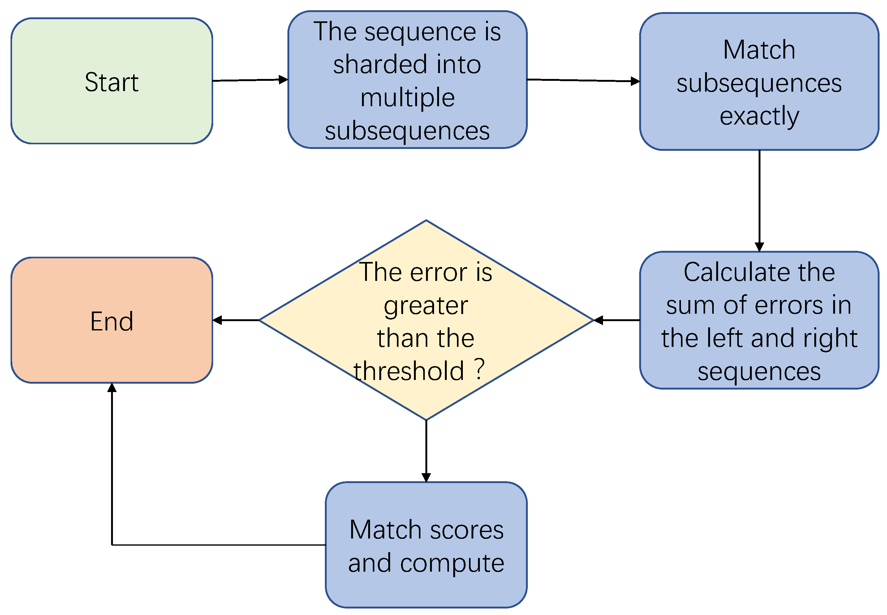For device fingerprint Finger, query pattern sequence q, and allowable error threshold $\tau$, fuzzy pattern matching is to find all subsequences $Trav[i,j]$ satisfying $sim(q,Trav[i,j\left]\right)$ ≤ $\tau$, where sim is Similarity function, where 1 ≤ i, j ≤ n, $Trav$ is the original sequence corresponding to the device fingerprint. The process of fuzzy matching is shown in the Figure 5. The sequence is first preprocessed to shard it into multi-segment subsequences, and then the multi-segment subsequences are accurately matched, and the error values between the matching sequence and the original sequence are counted. If the error value is higher than a certain threshold, it is directly judged that the matching failed, otherwise its matching score is calculated for the judgment of the final device. This section, we will first outline the overall process of fuzzy matching, then optimize the two processes of fragmentation and computing errors, and finally describe how to calculate the matching score of fuzzy matching.

If the query sequence q is divided into $\tau$ + 1 slices, because the error threshold is an integer, it is impossible for all $\tau$ + 1 slice sequences to have errors, and at least one slice sequence is an exact match. First, the query pattern sequence q is evenly divided into $\tau$ + 1 slices, and then all subsequences of the slice sequence that exactly match in the fingerprint sequence are found. For this work, please refer to Section 3.2. Considering a sharding sequence $q[i,j]$ of the query sequence q, the sharding divides the query sequence q into three parts $q[1,i-1]$, $q[i,j]$, and $q[j+1,n]$. The sequence can also be divided into three parts, $Trav[1,i-1]$, $Trav[i,j]$, and $Trav[j+1,n]$, which can be verified by checking the left and right subsequences, respectively. $Tra{v}_l^m$ and $Tra{v}_r^m$ represent the longest left and right extensions, respectively. First, Equation (5) is used to calculate the similarity between all suffixes of the longest extension on the left $Tra{v}_l^m$ and $q[1,i-1]$.

$$l=\underset{1\le i\le Tra{v}_l^m}{min}sim\left(q[1,-1],Trav[i,Tra{v}_l^m]\right)$$

(5)

Then, Equation (6) is used to calculate the similarity between all suffixes of the longest extension on the right $Tra{v}_r^m$ and $q[j+1,n]$.

$$r=\underset{1\le i\le Tra{v}_s^m}{min}sim\left(q[j+1,n],Trav[i,Tra{v}_r^m]\right)$$

(6)

If there is an approximate sequence $Trav[i,j]$ of the sequence q, then there must be $l+r\le \tau$. The time complexity of verification on the left and right is $O(\tau \ast (|q_l+q_r\left|\right))=O(\tau \ast (\left|q\right|-\left|p\right|\left)\right)$.

3.3.1. Sequence Sharding

The sequence fragmentation is involved in fuzzy pattern matching, and different fragmentation methods will also affect the performance of the algorithm. The most common sharding method is uniform sharding, the specific process is: first determine the length of each subsequence according to the total length of the sequence and the number of shards, and then cut evenly according to the length from the beginning of the sequence, so that the length of each subsequence is as consistent as possible. The advantage of this method is that it is fast, but there are certain shortcomings in slicing accuracy. For the query pattern sequence $q=issaapp,\tau =2$, if the uniform sharding strategy is adopted, it will be divided into three shard sequences of $iss,aa,pp$. For $Trav=mississippi$, shard iss has two exact matching subsequences on Trav, shard pp has one exact matching subsequence on Trav, and shard aa has no exact matching subsequence on Trav, all of which need to be verified. However, if it is divided into $issa,a,pp$, there is only one fragment sequence pp that exactly matches, and only needs to be verified once.

Definition 1.

Optimal k division: Given a fingerprint sequence $Trav$, a query sequence q and division number k, the optimal division of q is $P_B$, which satisfies Equation (7). $C(q,k)$ represents all sharding strategies that divide q into k shards. $G\left(p\right)$ represents the set of all k shards of the sharding strategy P. $w_s\left(p\right)$ represents the number of shard p appearing in $Trav$, that is, the weight of shard p.

$$P_B=\underset{p\in C(q,k)}{argmin}\sum _{p\in G\left(P\right)}{w}_s\left(p\right)$$

(7)

Enumerating all sharding schemes can find the optimal solution, but there are $\left(\genfrac{}{}{0pt}{}{\left|q\right|-1}{\tau }\right)$ strategies for dividing the query sequence q into $\tau +1$ slices, which is extremely inefficient. It will be better to directly divide q evenly. By observing the division strategy, it can be found that if $P=\left\{p_1,p_2,...,p_{\tau +1}\right\}$ is the optimal $\tau +1$ division of q, then $P^{\prime }=\left\{p_1,p_2,...,p_{\tau }\right\}$ must be the optimal $\tau$ partition of $q[1,k]$, where $k=|p_1|+|p_2|+...+|p_{\tau }|$. Therefore, a dynamic programming algorithm can be used to solve the optimal partition of q. In this paper, $w\left[i\right]\left[j\right]$ is used to represent the minimum weight for dividing $q[1,j]$ into i shards. $w[\tau +1]\left[\right|q\left|\right]$ represents the optimal solution for dividing the sequence q into $\tau +1$ slices, that is, the result. $w\left[i\right]\left[j\right]$ is initialized and updated with Equations (8) and (9).

$$w\left[i\right]\left[j\right]=w_s\left(q[1,j]\right)$$

(8)

$$w\left[i\right]\left[j\right]=\underset{i-1\le k\le j-1}{min}w[i-1]\left[k\right]+w_s\left(q[k+1,j]\right)$$

(9)

$w_s\left(q[k+1,j]\right)$ can be calculated using the exact matching algorithm in Section 3.2. The time complexity of calculating $w_s\left(q[k+1,j]\right)$ is $O\left(q\right[k+1,j\left]\right)$, the time complexity of computing all subsequence weights of q is $O\left(\right|q{|}^3)$. This process has high time complexity and can be further optimized. After calculating the weight of $w_s\left(q[k+1,j]\right)$, only $O\left(1\right)$ time complexity is needed to calculate $w_s\left(q[i,j]\right)$. Therefore, the suffix weight of $q[i,j]$ can be calculated from right to left, and the time complexity of this process is $O\left(j\right)$. At this time, the overall time complexity will be reduced to $O\left(\right|q{|}^2)$, and the time complexity of solving $W[\tau +1]\left[\right|q\left|\right]$ is $O\left(\right|q{|}^2\tau )$. In addition, an acceleration strategy can be adopted. If $W[i-1]\left[k\right]$ and $W[i-1][k-1]$ have the same weight, then $W\left[i\right]\left[j\right]$ does not need $W[i-1]\left[k\right]$ to be updated. Because $w_s\left(q[k+1,j]\right)\ge w_s\left(q[k,j]\right)$, there is $W[i-1]\left[k\right]+w_s\left(q[k+1,j]\right)\ge W[i-1][k-1]+w_s\left(q[k,j]\right)$, $W[i-1]\left[k\right]$ cannot be used to obtain smaller weights. Therefore, judgment conditions can be added in the dynamic programming process. If there is a group of consecutive units of equal value, they can be stored in a skip chain, and the calculation of these units can be skipped at one time, thereby improving the efficiency of the algorithm.

Two sharding algorithms, the uniform sharding strategy and the optimal sharding strategy, have been discussed above. Fragmentation using both algorithms is divided into three processes. The first step is sharding, the second step is query, and the last step is verification. The time complexity is shown in the

Table 3. Time overhead of sharding strategy.

	The Uniform Sharding Strategy	The Optimal Sharding Strategy
sharding	$O\left(\tau \right)$	$O\left(\right|q{|}^{\tau })$
query	$O\left(q\right)$	$O\left(q\right)$
verification	$O\left(\tau \right|q\left|W_E\right)$	$O\left(\tau \right|q\left|W_B\right)$

.

From the above table, it can be calculated that the cost difference between the two sharding algorithms is ${a\ast \left(\right|q|}^2\tau -\tau )+b\ast \tau |q|(W_B-W_E)$. a and b are the unit costs of the sharding phase and the verification phase, respectively, and $W_E$ and $W_B$ represent the weights of the uniform sharding strategy and the optimal sharding strategy, $W_E\le W_B$. When the cost difference is less than 0, that is, $W_B<W_E-a/b\left(\right|q|-1/\left(\right|q\left|\right))$, the optimal sharding strategy is better than the uniform distribution strategy. However, $W_B$ can only be calculated after determining the optimal sharding strategy. It is very inaccurate to determine which sharding strategy to choose by setting a threshold, and setting a fixed threshold in advance cannot adapt to the identification of different query sequences, which has poor flexibility.

This paper introduces a machine learning method to predict and select a segmentation strategy. After the device fingerprint is constructed in Section 3.1, a large number of query sequences with different lengths will be randomly generated, and then the cost of the two sharding strategies will be compared and labeled. The uniform sharding strategy has a small cost and is marked as 0, otherwise it is marked as 1. The problem is transformed into a binary classification problem. Four features are collected in this chapter, namely the length of the query sequence $\left|q\right|$, the number of shards $\tau +1$, the weight of the uniform division method $W_E$, and the weight difference of adjacent shards ${\sum }_{j=1}^{\tau }|w_s\left(p_{j+1}\right)-w_s\left(p_j\right)|$. The first two features are the basic information of the query sequence.

$W_E$ is the baseline value of overhead. ${\sum }_{j=1}^{\tau }|w_s\left(p_{j+1}\right)-w_s\left(p_j\right)|$ measures the probability of changing sharding to reduce overhead. When the value is small, it will favor the uniform sharding strategy. The training model adopts the support vector machine model (SVM). The main idea is to find a hyperplane that accurately distinguishes different sample data, and to make the Euclidean distance from the point closest to the hyperplane to the hyperplane as large as possible. The radial basis function kernel function (RBF) is used in the model training process, and the penalty factor C and the RBF kernel function coefficient g are obtained by grid optimization method to obtain the optimal value. After the model training is completed, the sharding strategy can be predicted and selected to improve the overall efficiency of the recognition algorithm.

3.3.2. Similarity Function

The most widespread way to measure the similarity of two sequences is based on the Levenstein distance, also known as the edit distance. It can achieve fault-tolerant matching of two sequences at the character level, and is also the similarity measure used in this chapter. It represents changing from one sequence to another with a minimum number of operations, including insertion, replacement, and deletion of characters. Given two sequences p and q, the similarity function based on edit distance is $leven$, $0\le leven(p,q)\le max(p,|q\left|\right)$. When $leven(p,q)\le \tau$ in the two sequences, where $\tau$ is the allowable error value above. The edit distance can be calculated by dynamic programming, as shown in Equations (10)–(13).

$$D(i,0)=i,(1\le i\le |p\left|\right)$$

(10)

$$D(0,j)=j,(1\le j\le |q\left|\right)$$

(11)

$$D(i,j)=\left\{\begin{array}{c}\hfill D(i,j-1)+1\\ \hfill D(i-1,j)+1\\ \hfill D(i-1,j-1)+C\left(p\right[i],s[j\left]\right)\end{array}\right.$$

(12)

$$C(x,y)=\left\{\begin{array}{c}\hfill 1,x\ne y\\ \hfill 0,x=y\end{array}\right.$$

(13)

Initially, the cell values in the first row and first column of the edit distance matrix are directly obtained by Equations (10) and (11), while other cell values can be obtained iteratively by Equations (12) and (13). For any unit on the edit distance matrix composed of sequence p and sequence q, $D(i,j)=ed\left(p\right[1,i],q[1,j\left]\right)$, so their edit distances satisfy $ed(p,q)=D\left(\right|p|,|q\left|\right)$, the time complexity of calculating the edit distance between two sequences is $O\left(\right|p|\ast |q\left|\right)$. In general, successful matches between sequences are rare. The above equation calculates the value of each column from top to bottom when updating the edit distance matrix. A cell value will soon be greater than $\tau +1$, where the surface is already mismatched. If the value of a cell is greater than $\tau +1$, the search results will not depend on this cell.

Based on the above conclusions, the algorithm can be further optimized. If the value of a cell in the edit distance matrix is less than or equal to $\tau$, the cell is called the active cell. When updating the edit distance matrix, it only needs to calculate the last active cell of each column and stop, and the value of its cells below will not be updated. In the process of device recognition, most of the recognition sequences and pattern sequences have a low degree of matching, and the number of updated active units is small, which can improve the recognition efficiency. The reason why this optimization algorithm is established is that the cost of insertion, deletion and replacement operations are all 1, so the difference between adjacent elements in the edit distance matrix is at most 1. This also limits the scalability of the recognition algorithm. In fact, various noises such as redundancy, disorder, and presence of noise in data traffic have different effects on device identification. Simply setting all operation overheads to 1 will reduce the accuracy of identification. In this paper, the generalized edit distance is used to improve the scalability and accuracy of the algorithm, that is, the cost of each operation is not the same, and the specific value is determined by the protocol and function.

Although the generalized edit distance can improve the correctness and scalability of the algorithm, it cannot be optimized in time, because the cost of each operation is not a fixed value, and the difference between adjacent unit values cannot be determined. The edit distance matrix needs to be completely updated each time to match with the device, which will waste a lot of time on meaningless calculations. In order to solve this problem, this paper proposes a diagonal jump algorithm for optimization.

3.3.3. Diagonal Jump Algorithm

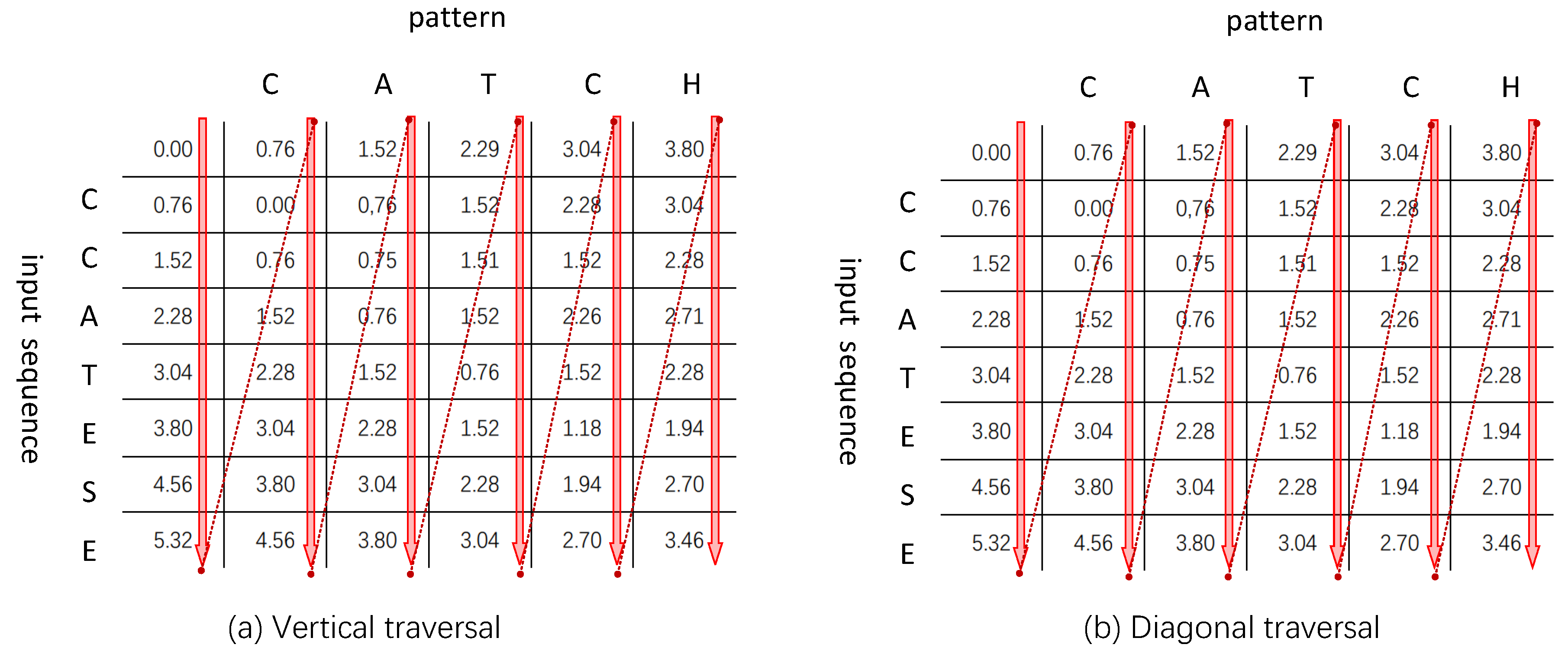
In this paper, the diagonal jump algorithm is adopted to avoid unnecessary cell value calculation. Different from the vertical traversal shown in Figure 6a, the edit distance matrix is updated using the diagonal traversal shown in Figure 6b.

Figure 6 shows the process of a diagonal traversal, where the arrows illustrate the order of steps computed in each traversal. In a diagonal traversal, the upper right cell value is computed before the lower left cell value. If $tra\left(t\right)$ is used to represent the value of a diagonal line, then $tra\left(t\right)$ needs to be updated by $tra(t-1)$ and $tra(t-2)$, and there is no dependency on the unit value inside $tra\left(t\right)$. When $tra(t-1)$ and $tra(t-2)$ are updated, the calculation of unnecessary unit values can be skipped when calculating $tra\left(t\right)$. Jump bitmaps are employed, avoiding multiple iterations during the loop without accessing all elements in the edit distance matrix. Each bit in the skip bitmap is assigned to a column of the edit distance matrix. When the trim bit of the column is set to “1”, the cell value of the column does not need to be updated in subsequent calculations. The specific steps are shown in Algorithm 3.

Algorithm 3 Diagonal jump algorithm

Input:$pattern:$ Sequence to be queried. $Trav:$ Original pattern sequence. $D\left[i\right]\left[j\right]:$ Edit distance unit value. $skip\_bitmap:$ Jump bitmap. $\tau :$ Maximum allowed error threshold. Output: $D:$ Edit distance matrix. 1: Initialize (D[i][0],D[0][j], $skip\_bitmap$). 2: for each $tra$ do 3:     for each step($\alpha$,$\beta$)2 $tra$ do 4:         if $skip\_bitmap$($\beta$) == 1 then 5:             Break 6:         end if 7:         if $skip\_bitmap$($\beta$) == 0 then 8:             D[$\alpha$,$\beta$]=costmin(D[$\alpha -1$][$\beta$],D[$\alpha$][$\beta -1$],D[$\alpha -1$][$\beta -1$]) 9:         else 10:            D[$\alpha$][$\beta$]=costmin(D[$\alpha -1$][$\beta$],D[$\alpha -1$][$\beta -1$]) 11:       end if 12:       if D[$\alpha$][$\beta$]>k and $skip\_bitmap$($\beta -1$) == 1 then 13:            $skip\_bitmap$($\beta -1$) = 1 14:         end if 15:     end for 16: end for 17: return D

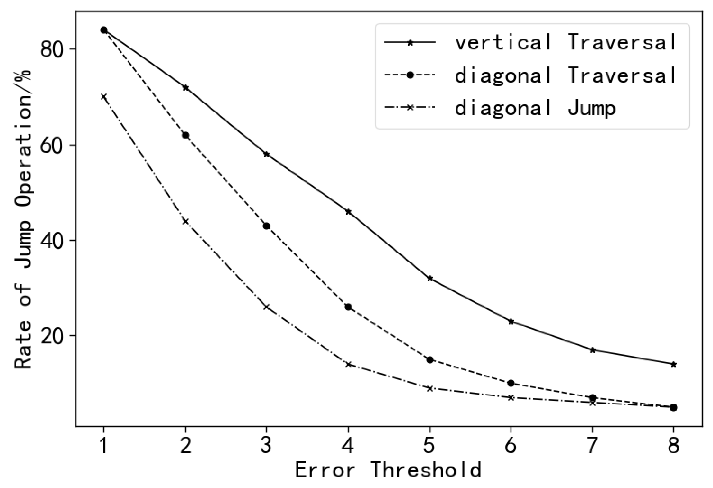
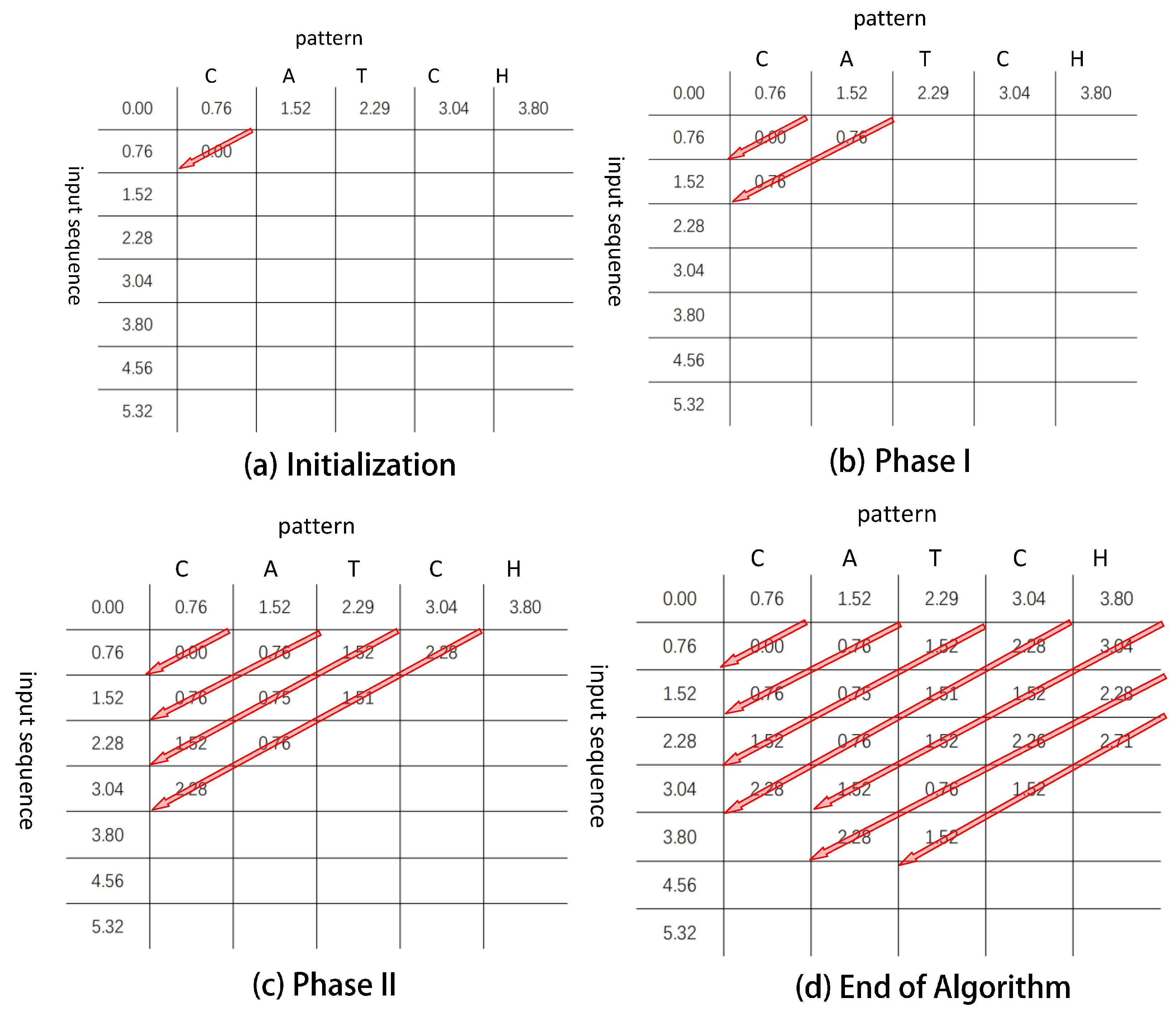
The number of diagonal traversals is proportional to the pattern sequence length j, so the time complexity is $O\left(jk\right)$. Figure 7 depicts the matrix update operation of the original sequence “ccatese” and the query sequence “catch”, with a threshold $\tau$ of 2. First, initialize the bit of the leftmost column in the skip bitmap to “1” and initialize $D\left[i\right]\left[0\right]$ and $D\left[0\right]\left[j\right]$, as shown in Figure 7a. When the fourth diagonal is updated, the cell value of the second column exceeds 2, as shown in Figure 7c. When traversing the fifth diagonal, since $skip\_bitmap\left(1\right)$ = 1, $D\left[3\right]\left[2\right]$ and $D\left[3\right]\left[1\right]$ will be used to update $D\left[4\right]\left[2\right]$, where the insert operation is skipped. Figure 7d shows the updated result of the final edit distance matrix. The diagonal skipping method proposed in this paper only needs to access the skip bitmap to determine which steps to skip without relying on previously updated data. In addition, the algorithm can skip the computation of multiple cell values and operations, thereby reducing the time of updating the edit distance matrix.

Through the above algorithm, the approximate matching position of the query sequence in the fingerprint sequence can be found, and then the matching score with the fingerprint sequence can be calculated according to Equation (14). The device with the highest matching score in the device fingerprint database is the identification result.

$$sc=\sum _{i\in match}\frac{100\ast |l_i-r_i|}{\sqrt{\frac{l_i\ast (1-l_i)}{2}+\frac{r_i\ast (1-r_i)}{2}}}$$

(14)

Among them, match represents the position where the query sequence approximately matches the fingerprint sequence. $l_i$ represents the similarity between the longest extension on the left and the left side of the shard at the ith matching position. $r_i$ represents the similarity between the longest extension on the right and the right side of the shard at the ith matching position.

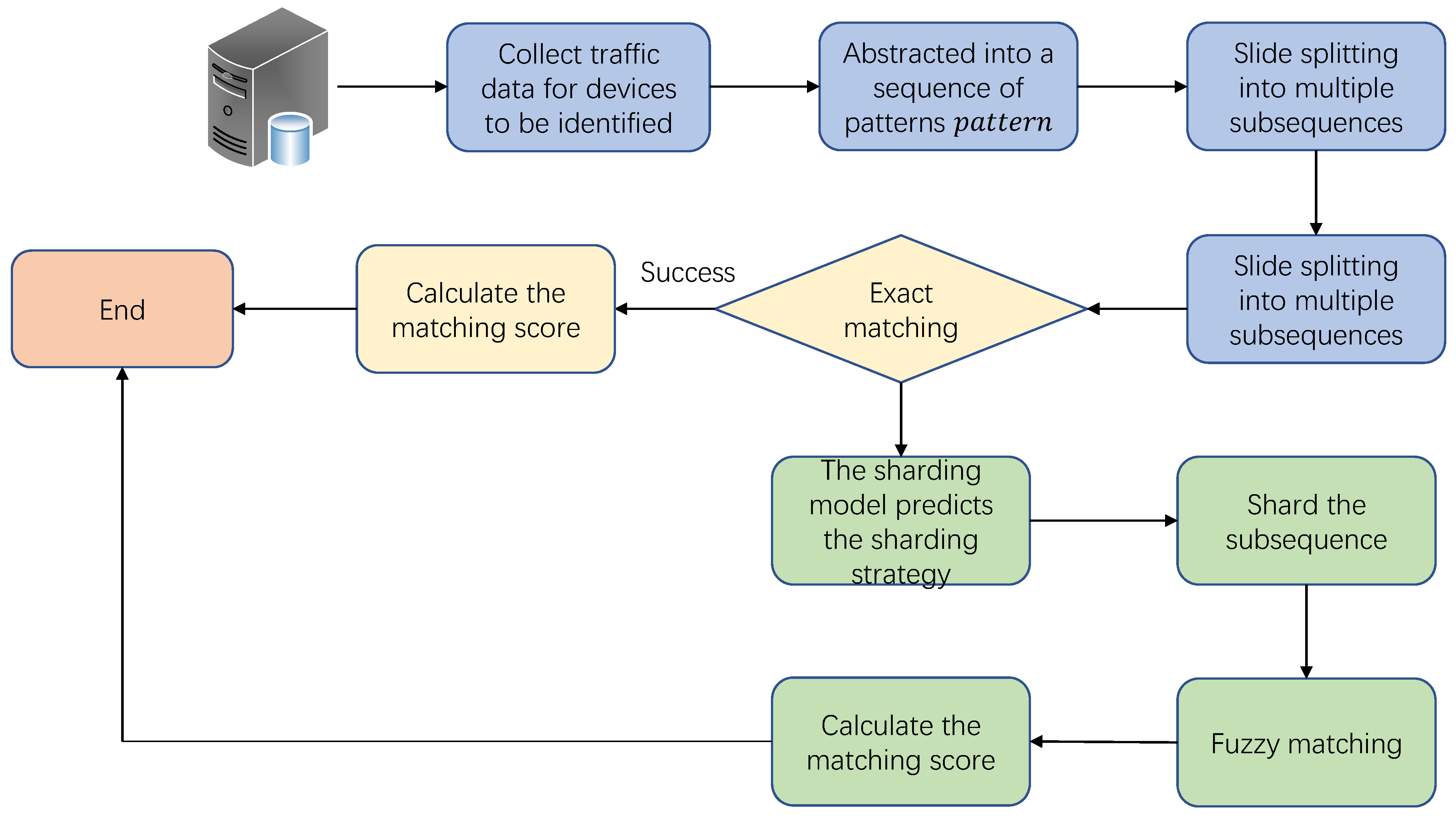
The device identification in this paper is based on a pattern matching algorithm, and the flow chart is shown in Figure 8. First try to use exact matching for the fingerprints in the device fingerprint database, but there is noise in the industrial control system, so the exact match often fails. In response to this situation, this paper uses the fuzzy pattern matching algorithm to further evaluate the matching degree, and the device with the highest matching degree is the recognition result.

4. Simulation Experiments

4.1. Comparing Models

This paper proposes an algorithm model for building a device fingerprint database and identifying unknown devices. The SA-IS algorithm is used to process pattern sequences as device fingerprints and store them in the device fingerprint database. When identifying an unknown device, the exact matching algorithm is first used to calculate the matching degree with the device fingerprint. If the exact pattern matching fails, the fuzzy pattern matching algorithm is used to evaluate the matching degree between the query sequence and the fingerprint. The device with the highest matching degree is the final recognition result. In order to evaluate the various indicators of the algorithm proposed in this paper, this paper will compare with SVM, random forest, and LSTM models.

Only one industrial control protocol is usually used during the operation of industrial control equipment, and many devices can be filtered out through the industrial control protocol used by unknown devices. Therefore, when training models such as SVM, different models will be trained for different industrial control protocols.

Among them, the SVM model and the random forest model are trained based on the features extracted from the traffic data, and a total of 64 features are extracted, including the field features of industrial protocols, timing features and TCP/IP features. LSTM is suitable for modeling time series data. In this paper, a sliding window is used to divide the abstract pattern sequence into multiple sub-sequences, which are labeled and input into the LSTM model for training.

This paper also evaluates the performance of the proposed diagonal skipping algorithm, and compares and analyzes the computational cost of matrix update for different algorithms under different error thresholds and similarity functions.

4.2. Experimental Environment

This section tests the performance of the device traffic fingerprint model and the diagonal jump algorithm. The experimental environment configuration is shown in

Table 4. Experimental environment configuration.

Name	Specifications
CPU	AMD Ryzen 7 4800H with Radeon Graphics
GPU	AMD Radeon(TM) Graphics
DRAM	16 GB
SSD	477 GB

.

4.3. Experimental Results and Performance Analysis

4.3.1. Performance Analysis of Diagonal Jump Algorithm

Figure 9a shows the average time required for different algorithms to update the edit distance matrix with multiple error thresholds $\tau$. At this time, the diagonal traversal algorithm has a longer average execution time than dynamic programming using vertical traversal due to the memory access overhead of conditional statements and reordering. In the experiments, the diagonal jump algorithm execution time increases as $\tau$ increases. When $\tau$ > 4, the execution time exceeds the time of vertical traversal, which means that when the threshold $\tau$ is large, the proposed method has no improvement over vertical traversal. Therefore, the proposed method can help reduce the execution time when the similarity function is the edit distance and the error threshold $\tau$ is small. Compared with vertical and diagonal traversal, when $\tau$ = 1, the execution time is reduced by 44.3% and 52.3%, respectively.

Figure 9b illustrates the average execution time when the similarity function is generalized edit distance. As is the case with the ordinary edit distance metric, the diagonal jump execution time increases as $\tau$ increases. When $\tau$ < 5, the average execution time of the proposed diagonal skipping method is shorter than that of vertical traversal, which means that in this generalized edit distance metric, many steps can be skipped when $\tau$ is small in computation. Diagonal traversal only increased the average execution time by 11.5% over vertical traversal. When $\tau$ = 1, the execution time of vertical and diagonal traversal is reduced by 55.7% and 60.3%, respectively. Further reductions in execution time are expected due to the smaller overhead of conditional statements and reordering memory accesses compared to evaluations using the edit distance metric.

Figure 10 depicts the rate at which the diagonal jump algorithm saves computational operations. The experiment counts two operations that save computational overhead when updating D[$\alpha$][$\beta$]. The first is that when skip_bitmap($\beta$ − 1) = 1, the insertion operation will be skipped, and D[$\alpha$][$\beta$] consists of D[$\alpha$ − 1][$\beta$] and D[$\alpha$ − 1][$\beta$ − 1] renew. The second is when skip_bitmap($\beta$) = 1, the cell value after the column exceeds the error threshold, so no update is required. When $\tau$ = 1, 70.9–84.6% of the step calculation is skipped. As $\tau$ increases, the proportion decreases rapidly, and with different similarity functions, the decrement rate may be different. When $\tau$ = 8, only 3.7–11% of step size computations can be skipped, where the overhead of conditional statements and reordering memory accesses increases the average execution time over vertical and diagonal traversals.

In fuzzy pattern matching, original sequence sharding, uniform sharding and optimal sharding are required. Uniform sharding has high efficiency, but the accuracy is not as good as optimal sharding. Reasonable selection of sharding algorithm can greatly optimize the time cost of matching. Therefore, this paper trains the SVM model for each device fingerprint to predict the fragmentation method of the query sequence. Figure 11 depicts boxplots of accuracy for building predictive models for different fingerprints under different industrial control protocols. For the Modbus protocol, most of the prediction accuracy is between 0.75 and 0.85, and a few prediction model accuracy is between 0.5 and 0.6. The model performs well on the s7comm protocol, with prediction accuracy between 0.85 and 0.9, and a few models with prediction accuracy between 0.65 and 0.75. The average precision of the prediction model based on the enip protocol component is about 0.8, the fluctuation is small and the outliers are close to the average. Therefore, building a fragmentation prediction model can effectively predict the fragmentation algorithm and save time overhead for subsequent fuzzy matching.

This paper conducts statistical analysis on the functional relationship between execution time and input parameters. The error threshold parameter $\tau$ of the experiment is set to 2. The similarity functions include generalized edit distance, shape similarity distance (shape), and keyboard distance (keyboard). In this paper, the regression method is adopted, and the lengths of the query sequence and the original sequence are used as input parameters, and the coefficient of determination ($R^2$) in the regression can be used to display the fitting degree of the regression model to the target data. When using edit distance, $R^2$ is only 0.267. When the similarity function is shape and keyboard, $R^2$ is 0.575 and 0.718, respectively. The results show that in addition to the input sequence and pattern length, other overheads can significantly affect the execution time of the Levenshtein distance metric.

Table 5. Regression statistical analysis table.

Function	Parameter	Coef	SE Coef	T	P
Edit Distance	Constant	2328.1	22.8	102.0	0
	Length1	34.0	1.7	20.40	0
	Length2	316.2	1.7	189.9	0
Shape	Constant	96.8	29.9	3.23	0
	Length1	64.9	2.2	29.17	$3^{-2}$
	Length2	803.4	2.2	366.9	0
Key Board	Constant	−52,085	329.1	−158.2	0
	Length1	1982.5	24.1	82.37	0
	Length2	15,981	24.0	664.9	0

lists the regression analysis results of the three similarity functions used, in which Coef., SE Coef., T and P represent coefficient, standard error coefficient, t-value and p-value, respectively, and length1 represents changing the query sequence Length, length2 means changing the length of the original sequence, and Constant means that the length of the sequence remains unchanged but the content changes. Because the p-value is small, it makes sense to count the length of the query sequence and the original sequence. The large t-value in Table 5 indicates that even if the query sequence and the original sequence have the same length, the execution time may vary greatly due to the difference in the contents of the two sequences. Furthermore, the coefficient of the original sequence length is more significant than that of the input sequence, which means that the pattern length is more critical in execution time.

4.3.2. Performance Analysis of Device Traffic Fingerprint Model

The data set used in the experiment in this section is the traffic data collected from the actual industrial control system. There are thousands of industrial control devices. However, during the experiment, it is found that many devices are clearly differentiated, which is of no help in evaluating the recognition ability of the model. Therefore, this article selects ten devices on three common industrial control protocols, including Modbus protocol, s7comm protocol and enip protocol. The traffic data collected from these devices are similar and indistinguishable, and experiments based on these devices can well evaluate the recognition ability of the model, and all experiments are conducted under the error threshold $\tau$ = 3.

Figure 12 describes the relationship between the recognition accuracy of each model and the number of devices in different industrial control protocols. Accuracy refers to the ratio of the number of correctly classified samples to the total number of samples. Figure 12a shows that the device traffic fingerprint model has the highest recognition accuracy. The highest accuracy rate is about 0.99, and the lowest accuracy rate is about 0.97. As the number of device fingerprints increases, the accuracy rate tends to decrease. Figure 12b,c are graphs of random forest and SVM models, respectively. Overall, the accuracy of random forest is slightly higher than that of SVM, but the accuracy of both models drops off a cliff when the number of devices is 7. Because the device configurations in the same industrial system are similar, the newly added device has almost the same characteristics as a previous device, so the trained model recognizes both devices as one, resulting in a drop in accuracy. When the number of device fingerprints is greater than 7, the accuracy rate is slightly improved, because the recognition accuracy of the newly added device is relatively high, which reduces the impact on the identification confusion of the two devices. Figure 12d is a graph of the LSTM model. The recognition effect is relatively stable, but the accuracy is slightly worse than that of the device traffic fingerprint model. There is a large amount of noise in the actual industrial system, which will affect the recognition of the LSTM model.

In Figure 12, the recognition accuracy of devices using different industrial control protocols is also different. For LSTM and device traffic fingerprinting models, the problem is pattern abstraction. Different industrial control protocols have different formats and abstract functions. The s7comm protocol has a complex format and has obvious characteristic fields, which can accurately abstract data packets. The Modbus protocol has few feature fields, and the pattern sequences abstracted by different devices are highly similar, which will affect the recognition performance. There are obvious characteristic fields in the enip protocol, but the change rate of these fields is high, and the similarity of the pattern sequence abstracted by the same device in different time periods will be low, which will affect the recognition result. For SVM and random forest models, the features extracted from different industrial control protocols are not exactly the same, and the recognition results will also be different. More features that are helpful for recognition can be extracted from the s7comm protocol, so the recognition effect is optimal.

Figure 13 describes the relationship between the recognition accuracy of each model and the number of device fingerprints in different industrial control protocols. Merely calculating the accuracy rate is not enough to evaluate the recognition ability of a model. The accuracy rate can well reflect the model’s ability to distinguish negative samples. The higher the accuracy rate, the stronger the model’s ability to distinguish negative samples. The highest accuracy rate is the device traffic fingerprint model, which is between 0.9725 and 0.995. The accuracy of the LSTM model is slightly lower than that of the traffic fingerprint model, between 0.95 and 0.98. The accuracy rates of the random forest and SVM models are relatively low, and the accuracy rates drop significantly when the number of device fingerprints is 7. The reason is the same as the drop in accuracy rates. The results show that the device traffic fingerprint model has a strong ability to distinguish negative samples.

Figure 14 depicts the relationship between the recognition recall of each model and the number of devices for different industrial control protocols. Recall is a measure of coverage that measures how well a classifier can identify positive examples. The recall rate of the device fingerprint model is about 0.78–0.89, and the recall rate of the random forest model and the recall rate of the SVM model are about 0.71–0.82, but the problem of equipment confusion fluctuates greatly. The LSTM model still performs well in the recall rate, which is about 0.02 different from the fingerprint model. The results show that the device fingerprint model has excellent performance in terms of recall rate and strong ability to identify positive samples.

Figure 15 depicts the ROC plots for the four models under the four devices. The abscissa is fpr, which indicates the proportion of samples that are predicted to be positive, but actually negative to all negative samples. The ordinate is tpr, which indicates the proportion of samples that are predicted to be positive and actually positive to all positive samples. The ROC curve combines the true positive rate and the false positive rate, which can accurately reflect the impact of any threshold on the generalization performance of the model, and help to choose the best threshold. The point on the ROC curve closest to the upper left corner is the best threshold with the least classification error, and the total number of false positives and false negatives is the least. The larger the area under the ROC curve, the better the performance of the model. From Figure 15a, it can be seen that the four ROC curves of the device fingerprint model are all close to the upper left corner, the highest area value is 1.00, the lowest is 0.94, and the comprehensive area value is 0.98. The performance of the random forest model and the SVM model is slightly worse, with the comprehensive area values of 0.94 and 0.92, respectively. The LSTM model still shows good performance, the highest area value is 0.97, the lowest is 0.96, and the comprehensive area value is 0.97, which is very close to the recognition effect of the device fingerprint model.

In the above experiments, the device fingerprint model shows excellent performance in terms of accuracy, precision, recall and ROC curve. The performance of random forest is slightly stronger than that of the SVM model, but it is inferior to the device fingerprint model in various indicators. The performance of the LSTM model is very close to the device fingerprint model, with a maximum difference of about 0.02 for each index. However, the amount of data required to train the LSTM model is large, and the model must be retrained when devices are added or removed, which has a large overhead.

As mentioned above, because there is a lot of noise in the industrial control system, the exact match is often not hit, and in the case of no hit, the fuzzy matching method is used for further identification. Figure 16 counts the number of exact matching and fuzzy matching used by device fingerprint model recognition devices. The highest proportion of exact matching in device identification is 0.213, and the lowest proportion is 0.0513, indicating that in most of the device identification process, precise matching cannot be a good hit, the fuzzy matching algorithm must be used for the final identification. Therefore, although the function of the device is stable, and the data packets sent and received are also periodic, the periodicity is not stable, and there are changes in different time periods. Therefore, it is not realistic to completely extract or match the periodicity. The matching proposed in this paper, which allows a certain fault tolerance, has better performance in practical systems.

Combining all the above experiments, the diagonal skipping algorithm proposed in this paper can skip a large number of calculation processes when the set error threshold is small, which saves the calculation overhead, and is very suitable for applications where the device fingerprint model sets a small error threshold. The device fingerprint model proposed in this paper performs well in terms of precision, precision and recall, and requires less data, so there is no need to retrain the model every time a device is added.

5. Conclusions

As industrial control systems gradually begin to access the Internet, their security issues have received widespread attention. At present, learning algorithms such as LSTM are often used in the industry for equipment recognition, but the recognition accuracy of such methods is not high, and it is necessary to waste resources to retrain the model regularly, waste resources, and have high complexity, which is not easy to deploy on embedded and other small devices. Combined with its device functions and periodic characteristics of traffic, this paper constructs a device traffic fingerprint database and device recognition based on the pattern matching algorithm, and also proposes diagonal jumping and optimal slicing algorithms to improve recognition accuracy and reduce time overhead. Finally, the experiment is carried out in the real production environment, and its recognition accuracy and overhead are better than the traditional algorithm. Therefore, the related methods proposed in this paper lay a solid foundation for the identification of industrial control equipment and provide new means for anomaly detection.