Feature Mining and Sensitivity Analysis with Adaptive Sparse Attention for Bearing Fault Diagnosis

Abstract

Bearing fault diagnosis for equipment-safe operation has a crucial role. In recent years, more achievements have been made in bearing fault diagnosis. However, for the fault diagnosis model, the representation and sensitivity of bearing fault features have a great influence on the diagnosis output results; thus, the attention mechanism is particularly important for the selection of features. However, global attention focuses on all sequences, which is computationally expensive and not ideal for fault diagnosis tasks. The local attention mechanism ignores the relationship between non-adjacent sequences. To address the respective shortcomings of global attention and local attention, an adaptive sparse attention network is proposed in this paper to filter fault-sensitive information by soft threshold filtering. In addition, the effects of different signal representation domains on fault diagnosis results are investigated to filter out signal representation forms with better performance. Finally, the proposed adaptive sparse attention network is applied to cross-working conditions diagnosis of bearings. The adaptive sparse attention mechanism focuses on the signal characteristics of different frequency bands for different fault types. The proposed network model achieves better overall performance when comparing the cross-conditions diagnosis accuracy and model convergence speed.

1. Introduction

With the intelligent development of mechanical equipment, high speed and heavy load have become the main characteristics of the modern mechanical system. Rolling bearings play a vital role in the operation of rotating machinery. They are widely used and easy to be damaged, thus it is necessary to monitor and diagnose their condition [1,2].

In the past few decades, studies on the evaluation of mechanical health status based on vibration signals have appeared frequently in the literature [3]. Generally, signal processing methods [4,5,6,7]—such as available time and frequency domain analysis, wavelet analysis, local wave analysis, and load identification in order to extract the signal characteristics and accomplish the goals of analysis and diagnosis, although the mechanical system is complex with interrelated subsystems—lead to the determination that the fault signal representation is not a one to one correspondence as it consists of various components, making traditional signal processing methods difficult for extracting effective features. However, data-driven deep learning methods can adaptively extract signal features and provide accurate diagnosis results. Therefore, deep learning-based methods of fault diagnosis have been applied more and more [8,9,10,11,12,13,14].

Despite the fact that deep learning has led to numerous research successes in the field of fault diagnosis, it is difficult to explain or visualize the process of result realization and output due to the layered architecture formed by stacking nonlinear processing units. Moreover, the model has weak explanatory power; thus, it is called the “black box” method [15]. The deep model’s potential for use in industrial field equipment fault diagnosis is severely limited as a result. Therefore, some researchers try to add attention mechanisms to the network in order to explore the interrelationship of data in the black box and hidden features that are currently difficult to find.

At present, the attention mechanism has been widely applied in the fields of text translation [16], speech recognition [17], document classification [18], etc. In the field of fault diagnosis, Li et al. [19] searched for important feature segments of signals by combining neural networks and attention mechanisms. Yang et al. [20] improved the interpretability of networks by combining the convolutional neural network model of the recursive gated unit and attention mechanism, and its visualization effect was verified on bearing datasets. According to the classification of literature [21], the above attention mechanisms are classified as soft attention. This kind of algorithm uses the weighted average of all the hidden states of the input sequence to construct the content vector. The application of the soft weighting method makes it easy for neural networks to learn effectively by back propagation, but it also leads to the cost of a second calculation. Xu et al. [21] proposed the hard attention model, in which the content vector is calculated by sampling the hidden state according to the probability of the input sequence, which significantly reduces the cost of calculation. However, its framework is not differentiable, and it cannot use the back propagation method for the iterative calculation. To achieve gradient back propagation, the Monte Carlo Sampling method is used to estimate the gradient of modules. Vaswani et al. [22] creatively proposed that the Transformer’s attention structure replaces RNN, which can be processed in parallel to achieve higher computational efficiency and solve the problem of long sequence gradient disappearance. However, it requires computing the relationship between pairs of sequences, which consumes more computing resources.

Luong et al. [23] further developed the attention mechanism and divided it into the local attention mechanism and global attention mechanism. Similar to the soft attention mechanism, the global attention mechanism takes notice of all sequences in data, which makes the network have a large computation cost and leads to the degradation of network performance [24]. The local attention mechanism is a trade-off between the soft and hard attention mechanisms. The network focuses on the area near the target sequence and reduces the computation expense. However, the local attention mechanism ignores the connection between non-adjacent sequences, thus its application has certain limitations [24]. Xue et al. [24] proposed a gated attention mechanism to address the above problems, which includes the trunk network and the secondary network. The trunk network realizes global attention, and the secondary network adopts a gated mechanism to select the sequence to be paid attention to in order to assist the attention sequence of the trunk network. However, in the literature [24], the input of the secondary network is consistent with that of the trunk network, which also leads to a larger parameter scale and additional computing costs. Zhao et al. [25] added a tiny filtering module in the deep network to generate soft thresholds through the attention mechanism to filter out unimportant information about features and significantly boost the performance against noise. The inputs of this module are channel characteristics after global maximum pooling; hence, the increase of parameters and computation cost is minimal. However, the filtering of the network is aimed at the internal characteristics of the channel, and all the sequences are still involved in the calculation, which cannot significantly reduce the network’s cost. At the same time, the operation of soft threshold filtering in the literature [25] is closer to the hard threshold method, which cannot be calculated by the back propagation method and needs to be optimized by a reinforcement learning strategy. To solve this problem, the gated attention network [24] uses the method of Gumbel-Softmax to simulate Bernoulli binomial distribution to achieve the calculation purpose of back propagation. Fu et al. [26] provided a mask function in line with the principle of back propagation in the target detection task, which can approximately simulate Bernoulli binomial distribution.

In this article, a new method, Adaptive Sparse Attention Network (ASAN), was proposed by borrowing the idea of soft threshold filtering in [25] and combining the advantages of global and local attention mechanisms. A network using the convolution of the neural network feature extraction ability and a two-way LSTM network has the advantages of dealing with long time-series data. Based on this added adaptive sparse attention module, the module generated a soft threshold adaptively by learning and using the threshold value filtering on the attention coefficient, removing unimportant sequence features and achieving the goal of sparse attention. The test and visual analysis are carried out on the CWRU bearing dataset and compared with the existing research. The outcomes indicate that the proposed ASAN method has better interpretability and higher training efficiency on the premise of keeping the model’s performance intact. It is important to note that although the CWRU bearing dataset is not difficult to classify and most models can achieve good results on this dataset, it is difficult to reflect the difference in model performance through it. However, it is still of great value to obtain the fault information distribution in data by exploring and verifying the feature extraction process of the model, especially in the current state of insufficient exploration of the explicability of the deep learning model.

The following are this paper’s contributions:

• A new adaptive sparse attention network, ASAN, is proposed, which uses a soft threshold to filter attention weight sequences and ignores redundant sequences through sparse operation, thus paying more attention to corresponding features.
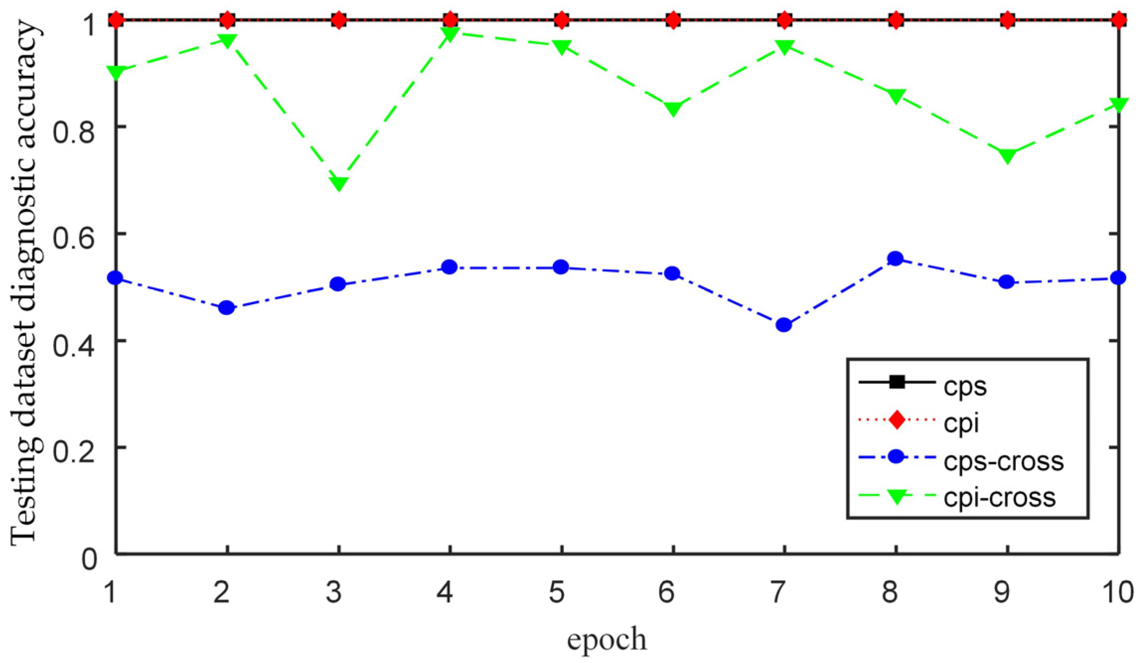
• Considering the influence of the independent and shared settings of the convolution parameters of each sequence on network performance, the comparison results of the cross-condition diagnosis performance show that the diagnosis method with the independent settings of the convolution parameters of each sequence has better generalization.
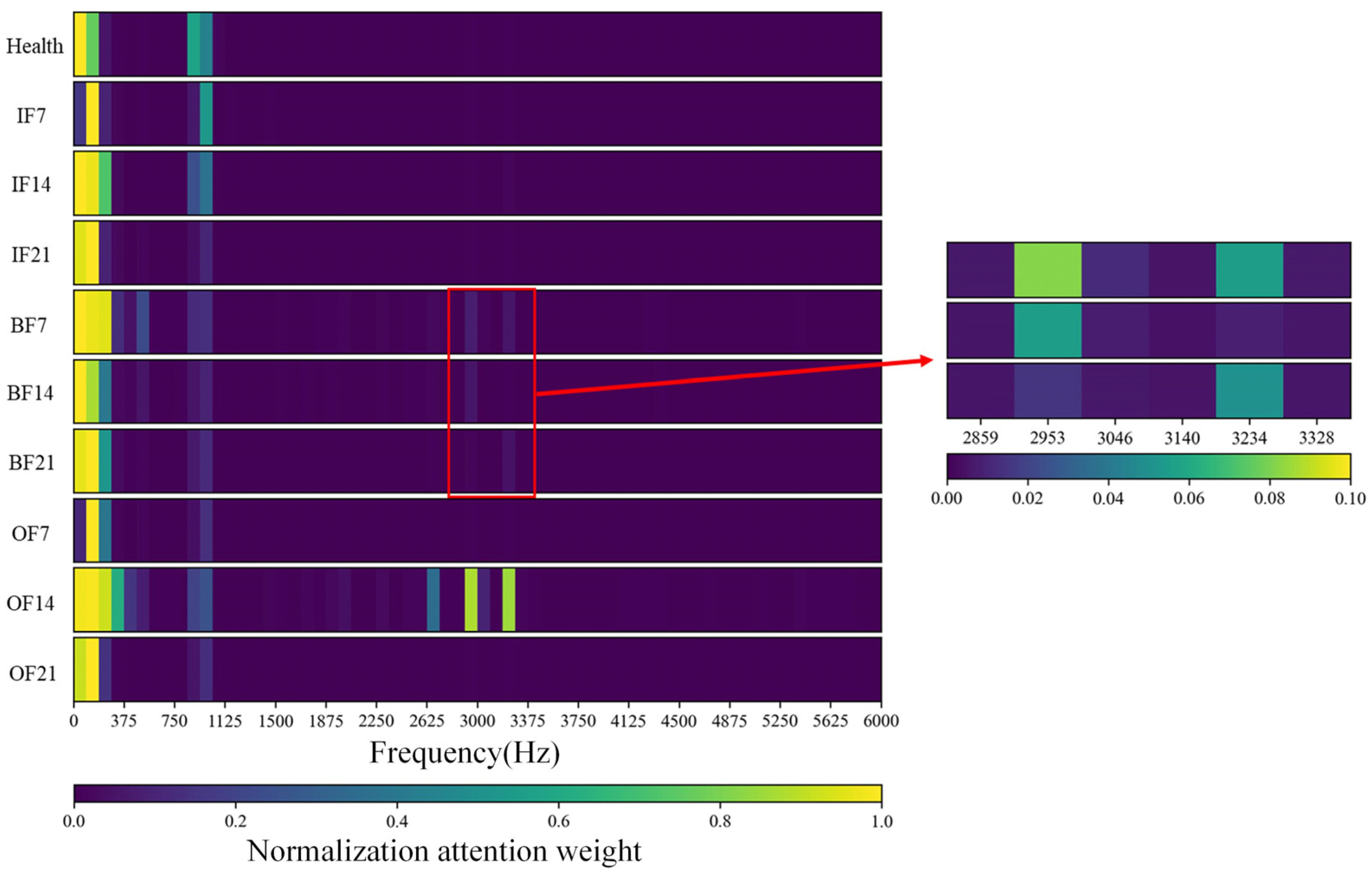
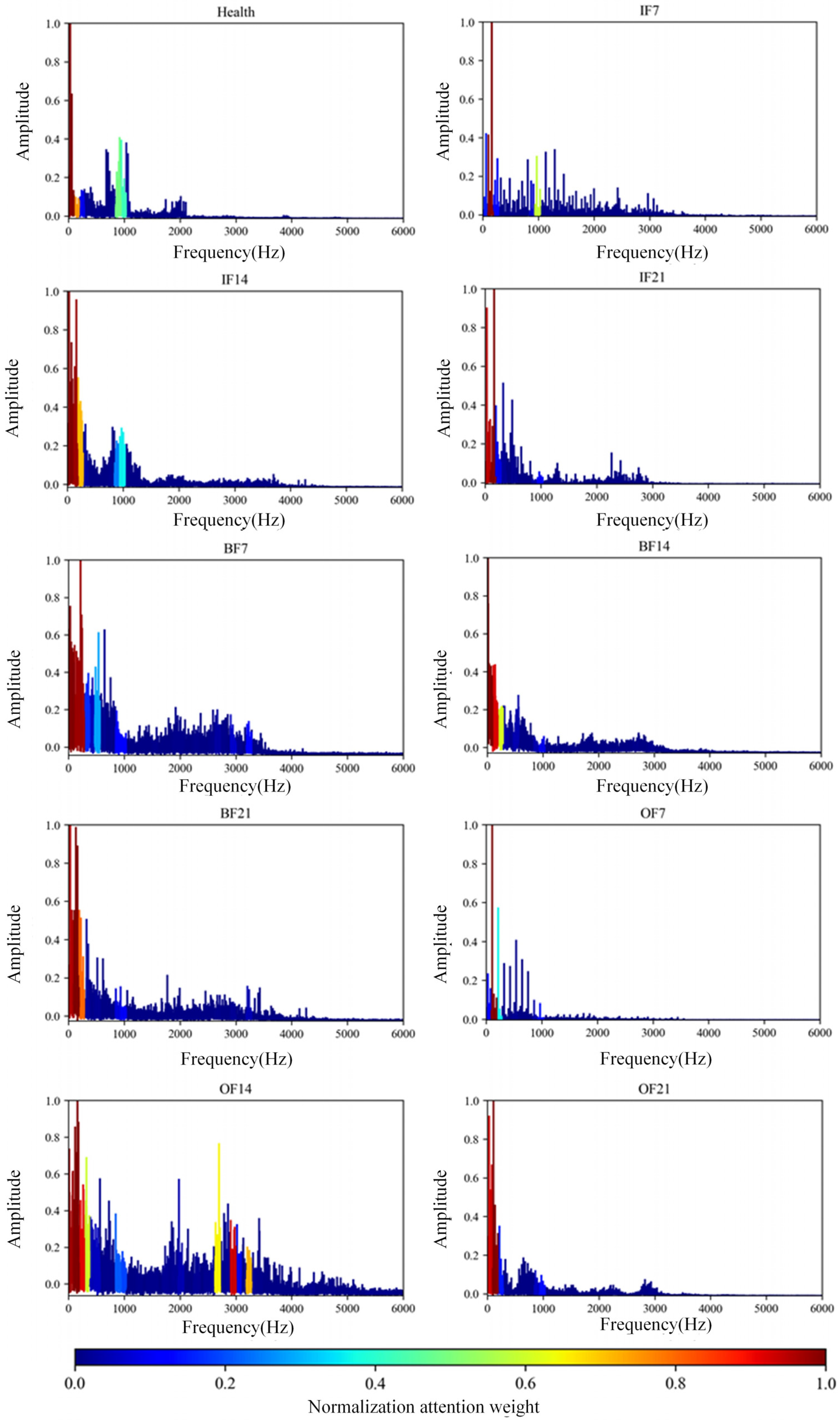
• The effectiveness of the proposed algorithm is verified on the CWRU bearing dataset. The attention mechanism mainly captures 1I, 1I side frequency, 6I of IF, 1-3x, 1B, 2B of BF, and 1O, 2O, 3O of OF, which is consistent with the rule of fault diagnosis knowledge (IF is the inner ring fault, BF is the ball fault, OF is the outer ring fault, 1X is the power frequency of the bearing, 1I is one time of the characteristic frequency of the bearing with inner ring fault, and 1B and 1O are the same). The proposed method can locate the fault feature region and has better interpretability and visualization effect.

The remainder of the paper is organized in the following way. Section 2 briefly introduces the theory of convolutional neural networks, BiLSTM networks, and attention mechanisms. Section 3 describes the specific structure of the proposed model and the fault diagnosis process. Section 4 discusses the obtained results through comparative validation. Section 5 concludes the paper.

2. Introduction of Relevant Basic Models

This section presents the theoretical principles of the basic network layers used in the proposed model. The proposed model first extracts the primary features of the signal sequence by the convolutional layer. Next, it extracts the long sequence signal features by the BiLSTM layer to capture the dependency between the before and after time features. Then, it focuses on the important features via the sparse attention mechanism. Finally, it completes the fault diagnosis via a softmax layer. Therefore, the basic network layers of the proposed method include the convolutional layer, the BiLSTM layer, and the attention mechanism layers. They are described as follows.

2.1. Convolutional Neural Network

The Convolutional Neural Network (CNN) is one of the typical neural network structures at present. CNN has good data feature extraction capability without excessive data preprocessing. Moreover, CNN is widely used in natural speech processing and image recognition due to its characteristics of local receptive field, spatial subsampling, and weight sharing [26,27,28,29,30]. In this study, for vibration signals or frequency domain signal sequences, 1DCNN is used for feature extraction, which is briefly introduced below.

Suppose the input data sequence is $x=\left[x_1,x_2,\dots ,x_n\right]$, where N is the length of the sequence, the length of the convolution kernel is $1\times l_k$, and the sliding step is s, then the sequence intercepted when the convolution kernel slides i step on the input sequence is $X_i=\left[x_{i\ast s+1},x_{i\ast s+2},\dots ,x_{i\ast s+l_k}\right]$. Finally, the convolution operation can be defined as:

$$z_{ij}=f({{\displaystyle \sum }}_{iϵN_s}{\mathrm{X}}_i\otimes K_j+b_j),$$

(1)

$$N_s=\frac{N-l_k}{s}$$

(2)

where the output $z_i$ is the feature learned by the convolution kernel during the sliding i step, $\otimes$ is the convolution operation, $N_s$ is the sliding number, f is the nonlinear activation function, $K_j$ is the j convolution kernel, $b_j$ is the offset. Then, the characteristic graph of the j convolution kernel $z_j=\left[z_{1j},z_{2j},\dots ,z_{N_{s}j}\right]$ is obtained.

Typically, a pooling layer is added between adjacent convolutional layers to extract important local information and reduce the dimension of the output matrix. Common pooling layer operations include maximum pooling, average pooling, and L2 pooling. Finally, the convolutional neural network flattens the learned features to the full connection layer, which is used to integrate the abstract features extracted from the previous layers and realize the direct link between the output data and the CNN.

The operation of multiple convolutional kernels enhances the ability of network data extraction, while multiple convolutional layers and pooling layers improve the learning ability of the CNN. The reasonable setting of CNN network parameters enables the CNN to better learn fault diagnosis knowledge.

2.2. BiLSTM Network

Bearing vibration acceleration time series contains rich state information. Recursive analysis of the time series can help extract the periodic response characteristics [31,32]. The recursive neural network (RNN) includes feedback connections between its hidden layer and the layer before it [33], and it has the ability to process sequential information. RNN can be trained using back propagation with target output and sequence input data.

For the input sequence $x=[x_1,x_2,\dots ,x_N]$, RNN hidden state vector calculation sequence $h = [h_1,h_2,\dots ,h_N]$, the output sequence $y=\left[y_1,y_2,\dots ,y_N\right]$, through the iterative equation below, from t = 1 to N.

$$h_t=f\left(w_{xh}{x}_t+w_{hh}{h}_{t-1}+b_h\right)$$

(3)

$$y_t=w_{hy}{h}_t+b_y$$

(4)

The w is the weight matrix and the b is the offset term. Where $w_{xh}$ represents the weight matrix for transformation between the hidden layer and the input layer, and $b_h$ is the offset vector of the hidden layer. The f is the nonlinear activation function of the hidden layer.

In general, $\gamma$ can be a sigmoid function in RNN. However, RNN’s performance suffers significantly as a result of the gradient disappearance issue during back propagation, which indicates that RNN may not be able to effectively capture long sequence data features. Therefore, a long- and short-term memory architecture (LSTM) was proposed to model the dependency between long sequences and prevent the problem of gradient disappearance in back propagation [19].

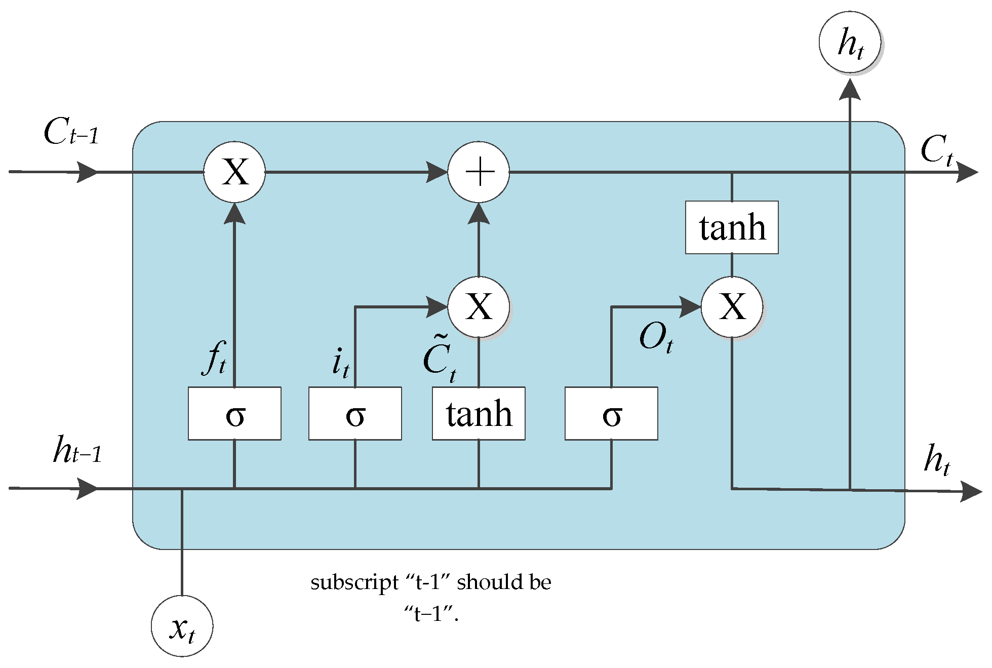
Figure 1 shows the LSTM operation process. The core idea of LSTM lies in its memory unit, which is an accumulator of state information. The LSTM has the ability to add or remove information from the cellular state, and this fine-tuning is achieved through the structure of the “gate”. Among them, the input gate $i_t$ controls how much of the current network input $x_t$ is saved to the unit state $c_t$, the forgetting gate $f_t$ controls how much of the last moment’s unit state $c_{t-1}$ is reserved to the current moment $c_t$, and the output gate $o_t$ controls how much of the unit state $c_t$ is sent to the current output value $h_t$ of LSTM. The mainstream LSTM algorithm in [34] is adopted in this study, as shown in the following function:

$$i_t=\sigma \left(w_{xi}{x}_t+w_{hi}{h}_{t-1}+w_{ci}{c}_{t-1}+b_i\right)$$

(5)

$$f_t=\sigma \left(w_{xf}{x}_t+w_{hf}{h}_{t-1}+w_{cf}{c}_{t-1}+b_f\right)$$

(6)

$$c_t=f_t{c}_{t-1}+i_t\mathit{tanh}\left(w_{xc}{x}_t+w_{hc}{h}_{t-1}+b_c\right)$$

(7)

$$o_t=\sigma \left(w_{xo}{x}_t+w_{ho}{h}_{t-1}+w_{co}{c}_t+b_o\right)$$

(8)

$$h_t=o_t\mathit{tanh}\left(c_t\right)$$

(9)

where $\sigma$ is the sigmoid activation function. Accordingly, the w matrix subscript in the formula is easy to understand. For example, $w_{hi}$ represents the matrix of transformation between the input gate and the hidden layer, $w_{xc}$ represents the matrix of transformation between the input state and the output gate, etc. With LSTM, the back propagation gradient can be captured in memory cells to prevent rapid loss.

LSTM assumes that the current time step is determined by the sequence of previous earlier time steps; thus, it passes information forward and backward through hidden states. Sometimes, the current time step may also be determined by subsequent time steps. If LSTM can keep an eye out for both front and back information, the network will better mine the characteristic information of vibration signals.

Bidirectional RNN realizes bidirectional information transmission by setting two parts: forward hidden information $\overrightarrow{h}$ and backward hidden information $\overleftarrow{h}$. The iterative updating process of the output layer is as follows:

$${\overrightarrow{h}}_t=\gamma (w_{x\overrightarrow{h}}{x}_t+w_{\overrightarrow{h}\overrightarrow{h}}{\overrightarrow{h}}_{t-1}+b_{\overrightarrow{h}})$$

(10)

$${\overleftarrow{h}}_t=\gamma (w_{x\overleftarrow{h}}{x}_t+w_{\overleftarrow{h}\overleftarrow{h}}{\overleftarrow{h}}_{t-1}+b_{\overleftarrow{h}})$$

(11)

$$y_t=w_{\overrightarrow{h}y}\overrightarrow{h}+w_{\overleftarrow{h}y}{\overleftarrow{h}}_t+b_y$$

(12)

Bidirectional LSTM can be realized by incorporating LSTM into the bidirectional RNN framework.

2.3. Attentional Mechanism

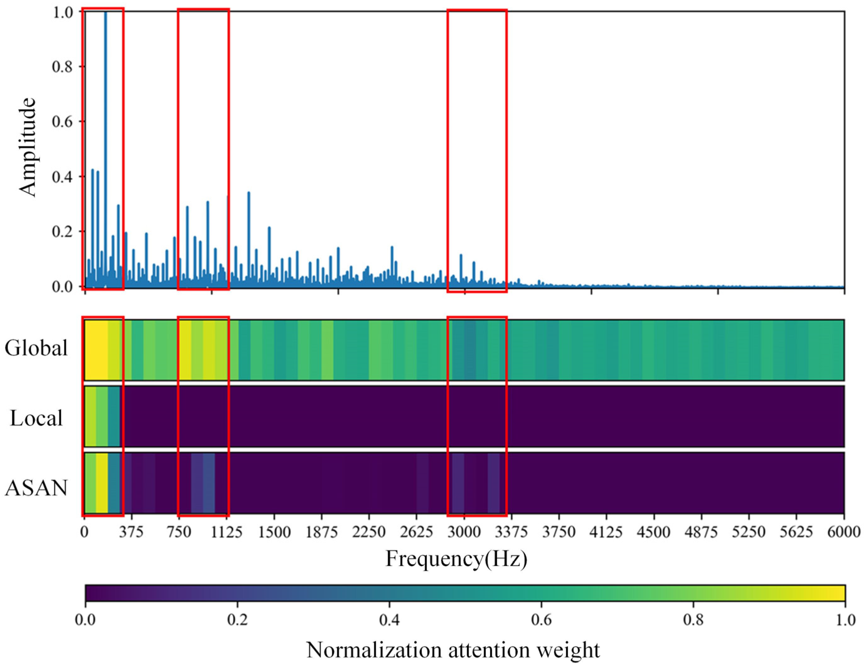
It has been widely pointed out in the literature that different segments in the spectrum contribute differently to fault characteristics. This inspired the use of attentional mechanisms. In this study, the segmented spectral sequence signals are used as input, and an attention mechanism is employed to generate an attention coefficient for each segment sequence, which enhances or weakens the characteristics of a segment signal by weighting the product. The attention weights are also visualized to locate the frequency domain interval segment where the fault information is located, which is consistent with the mechanism of increasing the amplitude of the rotational frequency and its multiples in bearing fault diagnosis.

The computational process of the attentional mechanism can be described as follows:

$${\alpha }_i=softmax(s\left(x_i,q\right))=\frac{exp\left(s\left(x_i,q\right)\right)}{{{\displaystyle \sum }}_{j=1}^N\left(s\left(x_j,q\right)\right)}$$

(13)

Among them, ${\alpha }_i$ represents the degree of correlation between the ith input sequence and the ith query sequence, that is, the ith attention coefficient. $s\left(x_i,q\right)$ represents the attention scoring function, which is used to calculate the correlation between the input sequence and the query sequence. $x=\left[x_1,x_2,x_3,\dots ,x_N\right]\in R^{D\ast N}$ represents the input vector, and q represents the query vector.

Here, the query vector, key vector, and value vector are all hidden states of the input vector x. The query vector and key vector generate attention weight coefficients by the scoring function and then assign the coefficients to the corresponding value vector segments to enhance the signal representation by weighted fusion.

Different scoring functions can produce different attention mechanisms. The scoring function used in this paper is obtained from the following formula:

$$s\left(x_i,q\right)=q^{T}tanh\left(W{x}_i+b\right)$$

(14)

where W and b are the trainable weight matrices and bias terms respectively.

Finally, the enhanced representation of the input data $y_{att}$ is obtained by the following formula:

$$y_{att}={\displaystyle \sum }_{i=1}^N{\alpha }_i{x}_i$$

(15)

Then, the enhanced signal $y_{att}$ is used as the input for further diagnosis. The softmax classifier was used to complete the final bearing status classification.

$$y=softmax\left(W_f{y}_{att}+b_f\right)$$

(16)

where $W_f$ and $b_f$ are the weight matrix and offset term, respectively. The network output is interpreted as the probability of various classes [35], and the final fault classification diagnosis is carried out.

3. The Proposed Adaptive Sparse Attention Network (ASAN)

3.1. Adaptive Sparse Attention Network

The attention mechanism imposes a set of attention coefficients on the whole sequence. Among them, the attention coefficients imposed by the more important sequence segments are large, and the attention coefficients imposed by the unimportant sequence segments are small, thus enhancing the classification ability of the network. However, in the application of fault diagnosis, the attention coefficients are scattered to more sequence segments with less classification contribution. As a result, the attention model imposes more computing costs and focuses on more redundant information. To get around this issue, we propose an adaptive thinning attention method. Through a layer of nonlinear transformation layers, the adaptive learning attention threshold is used to filter out smaller attention coefficients to achieve the purpose of attention thinning. The process is as follows.

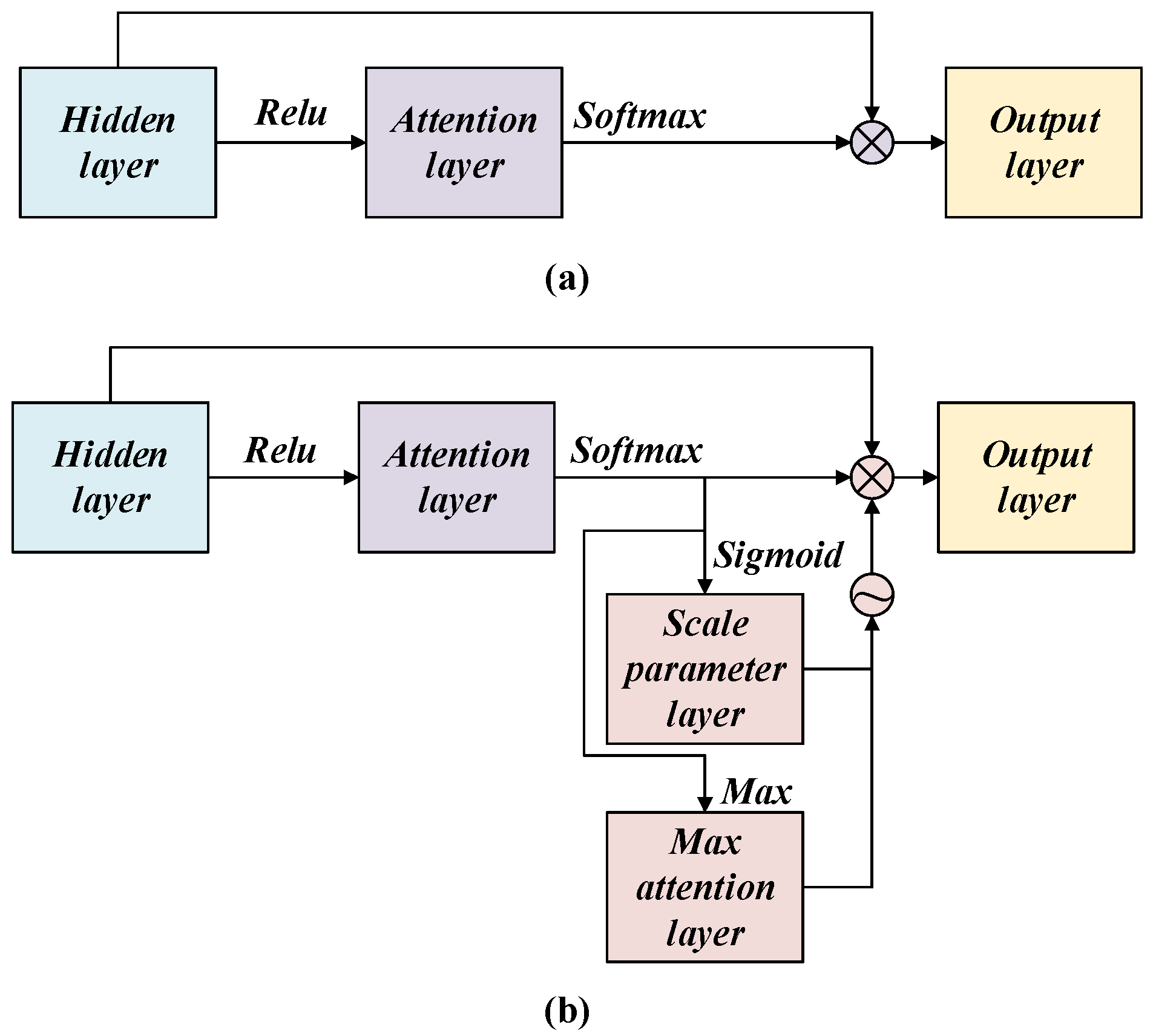
The typical attention structure is shown in Figure 2a, and the proposed adaptive sparse attention structure is shown in Figure 2b. This module adds a Scale parameter layer and a Max attention layer after the attention layer. The Scale parameter layer takes the output z of the attention layer as the input and finally generates a scale parameter $\alpha$. The calculation process is shown as follows:

$$\alpha =sigmoid\left(W_{\alpha }z+b_{\alpha }\right)$$

(17)

where $W_{\alpha }$ and $b_{\alpha }$ are the trainable weight matrix and bias terms, respectively.

The Max attention layer takes the output z of the attention layer and the output $\alpha$ of the Scale parameter layer as input, and an attention threshold is finally generated $\tau$. The calculation process is shown as follows:

$$\tau =\alpha \cdot \mathit{max}\left(z\right)$$

(18)

Then the natural exponential function is used to construct the filter function. The calculation process is as follows:

$$f\left(z\right)=\frac{1}{1+e^{-a\left(z-\tau \right)}}$$

(19)

Here, when $z<\tau$, the output result of $f\left(z\right)$ tends to be 0. When $z=\tau$, $f\left(z\right)$ equals 0.5. When $z>\tau$, $f\left(z\right)$ tends to be 1.

Last, the output of the threshold filter and the output of the attention layer are reconstructed with the softmax function to obtain the attention coefficient $new{z}_i$. The procedure for calculating is as follows:

$$new{z}_i=\frac{f\left(z_i\right)e^{z_i}}{{\Sigma }_{i=1}^{N_{seg}}f\left(z_i\right)e^{z_i}}$$

(20)

where $N_{seg}$ represents the number of sequences.

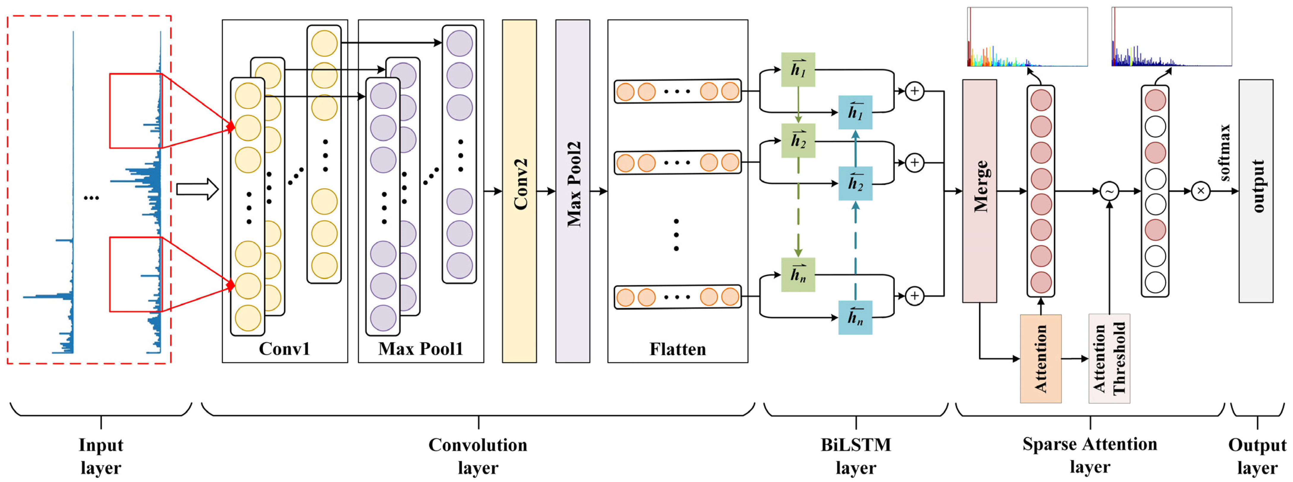
3.2. The Network Structure

The structure of the proposed deep network for fault diagnosis is depicted in Figure 3. To further illustrate, the bearing vibration envelope spectrum signal is used as the model input.

First, the input data sample is divided into $N_{seg}$ subsamples, i.e., $N_{seg}$ sequences, and each subsample contains $N_{sub}=\frac{N_{input}}{N_{seg}}$ data points (all adjusted to integers for the convenience of subsequent calculation). Next, the convolution layers Conv1 and Conv2 are used to extract features for each signal segment, and then the max-pooling operation is carried out. The two convolution layers use the same structure, but the parameters are slightly different. Multiple local convolutional kernels with a window length of $F_L$ are used for each layer respectively, and the zeroing operation is carried out to keep the dimension of the feature extraction layer unchanged. Each sequence signal’s spatial characteristics can be deduced in this manner.

Then, a full-connection layer was added to each segment of the signal for feature extraction, and softmax was used to assign attention weight to each segment of the signal. Subsequently, the attention weight is filtered by an adaptive threshold, and a sparse attention weight is obtained. Finally, the enhanced representation vector of the signal is created by multiplying the sparse attention weight by each segment signal.

After the signal is enhanced by sparse attention, all the sequence features are integrated into a bidirectional LSTM layer. The bidirectional LSTM can connect forward and backward hidden states to capture sequential information in the input data.

Dropout technology is a useful regularization technique that can prevent training data from being over-fitted. The authors of [36] recommended using dropout technology with a ratio of 0.4 at multiple levels of the network. In addition, the rectified linear unit (ReLU) activation function is generally used in the network. Because they do not have the problem of gradient disappearance or gradient diffusion during training, they can generally achieve better performance, especially in deep architectures [37]. Among them, the leaky ReLU first proposed is a variant of ReLU, which can be used as the attention module’s activation function to determine the difference in how attention weight is distributed. In this study, the cross-entropy function was used as the loss function [38]. The parameters of the proposed network are shown in

Table 1. Network parameter settings.

Parameters	Value
Number of training	300
Learning rate	0.001
Conv1 convolution kernel size	3
Conv1 number of convolution kernels	8
Conv2 convolution kernel size	3
Conv2 number of convolution kernels	16
LSTM hidden layer unit	16
Dropout	0.4

.

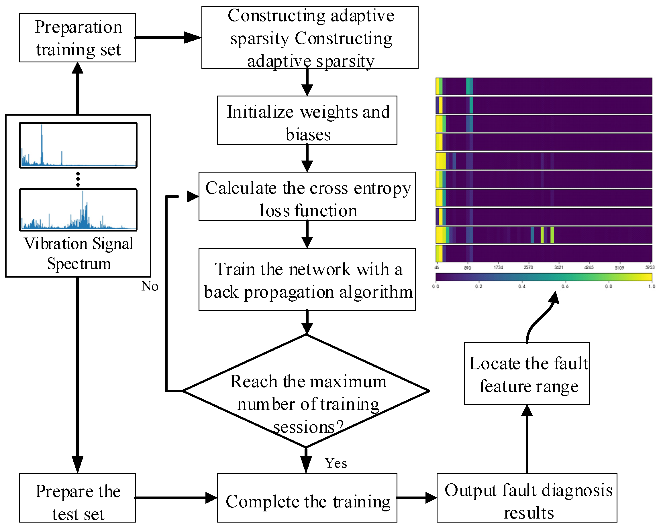
3.3. The Diagnosis Process

Figure 4 depicts the proposed fault diagnosis method’s flowchart. First, the original mechanical vibration signals are collected by sensors. Then, the vibration data are preprocessed to conform to the input format of the model, and training samples and test samples are made accordingly. The network obtains fault diagnosis results through training and learning, and the knowledge learned in the diagnosis process is well explained through corresponding visualization methods.

Next, the network configuration is selected from the architecture presented in Section 3.2, based on the information in the dataset and the particular issue with fault diagnosis. The detailed network structure includes the number of layers, the number and size of convolutional kernels at the convolutional layer, the number of neurons, etc., which are mainly determined by model verification in experimental research, with vibration data as the input of the model. Network biases and weights are initialized with the Xavier standard initializer.

The BP (Back-Propagation) algorithm was used to update all parameters in the network, and the target was minimized in small batches using the Adam optimization technique. The learning rate is 0.001, and after 300 training, the proposed network loss function converges on the whole. Table 1 displays the corresponding parameters.

Finally, the test fault diagnosis results are obtained by incorporating the test samples into the proposed model following the completion of the training phase. At the same time, the fault feature region that is most relevant to the result can be located through the model, which lays a foundation for the subsequent difficult fault research and diagnosis.

4. Model Analysis and Comparative Validation

4.1. Introduction to Dataset

This section validates the diagnostic effectiveness of the proposed method with the dataset provided by the Case Western Reserve University (CWRU) Bearing Data Center [39], and it is compared with other methods and related studies. In order to reduce the influence of randomness, the reported experimental results were averaged by 10 experiments. All experimental results were obtained on an Intel (R) Core (TM) i5-8400 CPU with 2.80 GHz and 16.0 GB RAM via TensorFlow and Keras. Python is used to complete the entire experiment. A photograph of the test stand is shown in Figure 5. The features of the measurement system are shown in

Table 2. The features of the measurement system.

Description	Functional Parameters
Electric motor	2 hp (1 hp = 746 W)
Torque transducer & encoder	Measuring torque and speed
Electronic controller	Adjusting torque
Signal type	Vibration acceleration signal
Data logger	16 channels
Sampling frequency	12,000 Hz
Measuring bearing position	drive end, fan end, base

.

This study uses the bearing data from the drive end of the test stand motor. The experiments were conducted on the bearing arrangement 3 o’clock, 6 o’clock, and 12 o’clock directions of failure, and vibration signals under four different health states were used: (1) Health state (Health); (2) Outer ring failure (OF); (3) Ball failure (BF); (4) Inner ring failure (IF). The fault sizes were 7, 14, and 21 mils (1 mil = 0.001 in). The specific settings of the test faults and classification labels are shown in

Table 3. Test fault setting.

Code of the Working Condition	The Fault Location	The Fault Size	Class Label
Health	Health	0 [mil]	1
IF7	IF	7 [mil]	2
BF7	BF	7 [mil]	3
OF7	OF	7 [mil]	4
IF14	IF	14 [mil]	5
BF14	BF	14 [mil]	6
OF14	OF	14 [mil]	7
IF21	IF	21 [mil]	8
BF21	BF	21 [mil]	9
OF21	OF	21 [mil]	10

. The one-hot encoding labels are used in the program. The operating loads were 0 and 3 hp in order to explore the cross-condition diagnostic performance of the model for working conditions. Therefore, the dataset contains 10 bearing health conditions under 2 loads.

Referring to [20], this section uses the envelope spectrum as the input signal, takes 8192 data points as a sample, normalizes the sample data, and divides the training set, verification set, and test set into 60%, 20%, and 20%, respectively. The test load and bearing fault characteristic frequency are shown in

Table 4. Test load and bearing fault characteristic frequency.

Load	Speed	IF	BF	OF
0 hp	1797 [rpm]	162.19 [Hz]	141.17 [Hz]	107.36 [Hz]
3 hp	1730 [rpm]	156.14 [Hz]	135.90 [Hz]	103.36 [Hz]

, and the calculation method of the bearing fault characteristic frequency is referred to in [40].

4.2. Weight Sharing and Weight Independent Comparison Test

Additionally, in order to study the influence of whether the weights in the convolutional layers of each sequence are shared in the performance of the model, two sets of control experiments are set up. The network model in Section 3.2 serves as the foundation for all experimental model structures, but the attention module is not included. Adjust the corresponding network model and conduct multiple experiments. Referring to [20], the dataset is preprocessed and its parameters are shown in

Table 5. Summary of the dataset parameters.

Parameters	Value
Number of Samples	500 (100%)
Number of train data	300 (60%)
Number of validation data	100 (20%)
Number of test data	100 (20%)
Number of features	8192
Number of Classes	10

. Further, each input sample is divided into 64 segments of equal length, and each segment of the signal contains 128 data points. The convolution parameters of each sequence in the first group of experiments are shared, denoted as CPS (Convolution parameter sharing); in the second group of experiments, the convolution parameters of each sequence are independent, denoted as CPI (Convolution parameter independence). The number of experimental data points in both groups is 8192, and the experimental dataset is under the condition of 0 hp load, including 10 fault settings shown in Table 3. In order to evaluate the model performance in various aspects, the network was trained using data from 0 hp load, and cross-case diagnostic tests were carried out under 3 hp load. Each group of experiments is repeated 10 times to reduce the impact of the randomness of the test results. The fault diagnosis accuracy and cross-working condition diagnosis performance are shown in Figure 6. The diagnostic accuracy is given in the manner shown in Equation (21).

$$accuracy=\frac{n_{TP}+n_{TN}}{n_{TP}+n_{TN}+n_{FP}+n_{FN}}\times 100\%$$

(21)

where $n_{TP}$ is the number of true positive samples, $n_{TN}$ is the number of true negative samples,$n_{FP}$ is the number of false positive samples,$n_{FN}$ is the number of false negative samples.

As can be seen from Figure 6 and

Table 6. Evaluation of test results for each test.

Experiment Method	Mean	Std
CPS	100.00%	0.00%
CPI	100.00%	0.00%
CPS-cross	50.80%	3.60%
CPI-cross	87.30%	9.00%

, the bearing data features are relatively clear, and the model classification performance can reach 100%, but the cross-working condition diagnosis performance of the CPI method is significantly better than that of the CPS method. Hence, the diagnostic generalization of the independent method of each sequence convolution parameter is better.

4.3. Model Performance Comparison

In order to confirm that the proposed adaptive sparse attention network is effective in fault diagnosis, various existing intelligent diagnosis methods and related research are compared and analyzed with the proposed method. Among them, in the BP method, the inputs are manual features and angular domain signals, and each layer has 4-10-7 and 3600-60-7 nodes, respectively. In the CPI method, the network structure described in Section 3.2 is used, the attention module is not included, and the convolution parameters of each sequence are independent. In the global method, the network structure described in Section 3.2 is used, but the structure of attention uses global attention. In the local method, the network described in Section 3.2 is also used, but the structure of attention uses local attention, that is, pays close attention to the target sequence’s window area, and the window contains 10 sequences. In the proposed ASAN method, the structure of the network is as shown in Section 3.2. Each method trained the model with angular domain (time domain), spectral, and envelope spectral data containing 10 fault settings under the same 0 hp load condition. As the diagnostic accuracy under the 0 hp load data reached 100%, the cross-working condition diagnosis test was carried out using the data of the 3 hp load, and the average accuracy of 10 cross-working condition diagnoses was calculated, as shown in Figure 7.

As depicted in Figure 7, the CPI, Global, Local, and ASAN methods are better than those on spectral and angular domain data in cross-working diagnostic performance on envelope spectrum data. However, the BP neural network method is more reasonable for fault diagnosis in the frequency domain, but the accuracy rate is only 48.8%, and the overall performance is poor. The CPI, Global, Local, and ASAN methods all greatly improve the cross-working condition diagnosis performance of the model. Among them, the ASAN method achieves the highest accuracy rates of 51.4% and 71.8% in the fault diagnosis of the angular domain and frequency spectrum, respectively. In the fault diagnosis of the envelope spectrum, the Global method achieves the highest accuracy rate of 98%, and the ASAN method achieves an accuracy rate of 97.6%, maintaining an excellent performance similar to the global method.

In order to further examine the proposed method’s efficacy, this study takes the envelope spectrum data as the input and takes the condition that the loss of the model training set no longer decreases as the model convergence. The convergence time of the CPI, Global, Local, and ASAN methods are counted as depicted in

Table 7. Diagnostic performance of different methods.

Diagnosis Method	Input	Diagnostic Accuracy	Diagnostic Accuracy across Working Conditions	Convergence Time (s)
CPI	Envelope spectrum	1	0.873	213.0368
Global	Envelope spectrum	1	0.980	389.7785
Local	Envelope spectrum	1	0.764	310.0060
ASAN	Envelope spectrum	1	0.976	196.5402

, and the trend of the training set loss of each method increasing with the epoch is shown in Figure 8.

It can be seen that the CPI method has a faster convergence speed and takes 213.0368 s to converge; Global enhances the model’s cross-condition diagnosis performance, but requires more computational cost. The Local method accelerates the model’s convergence, but it will lead to a decrease in the diagnostic performance across working conditions. Yet, the ASAN method only takes 196.5402 s of convergence time. Compared with other methods, it has a faster convergence speed and keeps up its excellent performance as global in fault diagnosis and cross-working-condition diagnosis. Taken together, the proposed ASAN method outperforms other algorithms in Table 7 to a certain extent.

To demonstrate the interpretability of the algorithm, the attention output of each sample is averaged, and Figure 9 shows the visualization results of each method.

As depicted in Figure 9, the global method mainly pays attention to the frequency around 0–1000 Hz and has second-level attention to the frequency components between 2000–3000 Hz, but the global method also has an attention weight of more than 0.4 for other frequency bands, which the interpretation of the model has a certain adverse effect. Due to the limitation of the window, the Local method can only concentrate on the low-frequency region, especially the 1-times frequency of the working frequency and the fault. After the sparse operation of the network, the ASAN method mainly takes notice of the low-frequency region, around 1000 Hz and 3000 Hz, which has a certain correlation with the attention weights obtained by the global method. However, the ASAN method can greatly suppress the expression of redundant sequences on the premise of ensuring the model’s performance, which can aid in our comprehension and diagnosis of fault signals.

4.4. Visualization of Fault Information

The fault form of the bearing is closely related to its fault characteristic frequency. The low frequency of the bearing fault characteristic frequency is often used in manual diagnosis. However, due to the modulation of the carrier wave, the fault frequency occasionally appears in the high-frequency region, which brings difficulties to manual diagnosis. Therefore, this paper uses sparse attention to further explore the performance of the fault characteristic frequency when the bearing fails. Figure 10 shows the average value of attention weights learned by the model for each bearing dataset working condition sample, and the visual attention weight of each working condition sample is depicted in Figure 11. The size of the attention weights is indicated by their color, and the red indicates the high level.

As shown in Figure 10 and

Table 8. Summary and average of attention weights for working conditions (where 1X represents 1 multiplier of power frequency, 2I represents 2 multiplier of IF, and so on) (The shade of the color represents the magnitude of the attention factor, with red representing a larger factor and green representing a smaller one).

Frequency Range	0–93.75	93.75–187.5	187.5–281.25	281.25–375	375–468.75	468.75–562.5	843.75–937.5	937.5–1031.25
health	1.000	0.762	0.055	0.010	0.007	0.009	0.581	0.440
IF	0.703	0.991	0.308	0.019	0.007	0.009	0.114	0.338
BF	0.987	0.948	0.626	0.062	0.025	0.098	0.079	0.115
OF	0.670	0.996	0.486	0.214	0.056	0.035	0.098	0.171
Corresponding eigenfrequency	1X, 2X, 3X	1I, 1B, 1O	2B, 2O	2B, 2I, 3O	3B, 4O	3I, 4B, 5O	6B, 8O	6I, 7B, 9O

, it is apparent that under the Health condition, the network pays attention to 0–281.25 Hz and 843.75–1031.25 Hz. When the inner ring of the bearing fails, the network mainly pays attention to the 1I and 6I frequencies of the bearing under the case of minor faults. Under medium faults, the network increases the attention of 1-3X, 1I side frequency, and 6I side frequency. Under severe faults, the network focuses emphatically on 1-3X and 1I. When the bearing rolling element fails, the network pays special attention to 2906.245–2999.995 Hz (21B) and the frequency range of 3187.505–3281.255 Hz (23B). In the case of minor faults, the network mainly pays attention to 1-3X, 1B, 2B, 4B of the signal, and it reduces the attention of most frequencies under moderate faults, especially the attention weights of 2B and 4B. The network attention position under serious fault is the same as that of medium fault, but the attention to 1B and 2B is increased. When the bearing outer ring fails, the network focuses on 1O and 2O under the case of minor faults. The network noticed multiple locations under moderate failures, focusing on 1-3X, 1O, 2O, 3O, 8O, 9O, and the high-frequency region (25O, 27O, 28O, 30O) near 3000 Hz. The attention of 1-3X is increased and the attention of 2O is reduced compared with that of minor faults in the case of severe faults.

In short, except for OF14, which obviously noticed the area around 3000 Hz, and the BF working condition, which slightly noticed the area around 3000 Hz, the attention weight differences of other signals were mainly concentrated in 0–562.5 Hz, 843.75–1031.25 Hz. The attention weights of each signal are summarized and counted in the above frequency domain interval according to the fault type, and the results are depicted in Table 8. Under the Health condition, the network mainly pays attention to 1-3X. Under the IF condition, the network mainly pays attention to 1I, 1I sideband, and 6I, which reduces the attention by 1-3X compared to Health, and also slightly pays attention to the 6I sideband. Under the BF condition, the network mainly pays attention to 1-3X, 1B, 2B, and slightly pays attention to 4B, 6B, 7B. Under the OF condition, the network mainly pays attention to 1O, 2O, and 3O. Compared with Health, the attention is reduced by 1-3X, and the attention is slightly paid to 8O and 9O. The network in [20] focuses on 1I of IF, 1B, and 2B of BF, and 1O, 2O, and 3O of OF, which is consistent with the attention results of the network proposed in this paper to a certain extent. This shows that the test results in this paper conform to the general rule of fault diagnosis knowledge.

5. Conclusions

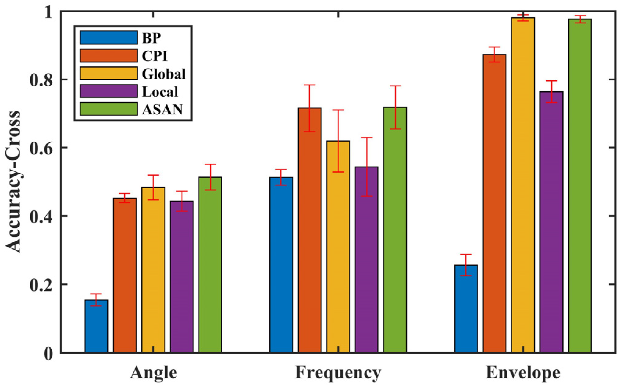
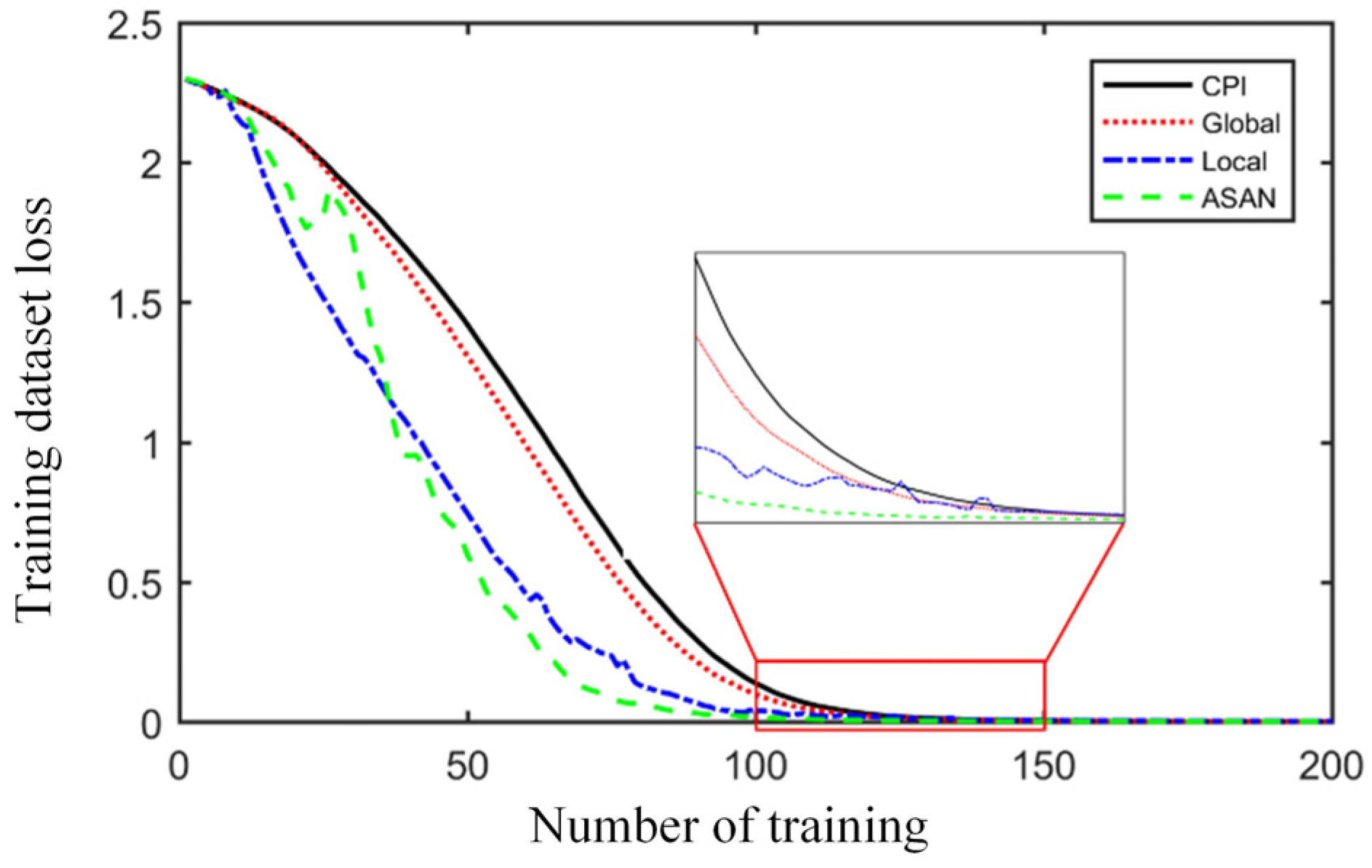
In this paper, a fault diagnosis model based on an adaptive sparse attention network is proposed. Through the soft threshold filtering of attention network weight, the diagnostic weight of the signals is adaptive and sparsely represented, and the signals of different representation domains are used as the model input for comparative analysis. The results show that the envelope spectrum of the bearing vibration signal has a more effective representation ability for fault information, and the proposed sparse attention model can automatically screen out the characteristic information that is more sensitive to faults. In addition, the proposed adaptive sparse network model achieves 97.6% accuracy and 196.54 s convergence time, which is 21.2% more accurate and 113.47 s shorter than the local method, and 193.24 s shorter than the global method, although the accuracy decreases by 0.4%. Therefore, the proposed model has better comprehensive performance, and the visualization has a better interpretation.

In the future, the knowledge screening network model can be used to further explore the differences in weights of sensitive features corresponding to different faults and their variation patterns with working conditions, etc., in order to provide directional guidance for an in-depth explanation of the fault mechanism and achieve the purpose of feedback maintenance. The problem of collaborative updating of the model and real-time data will be studied later and validated in real industrial fields.

References

1. Yang, J.; Wu, C.; Shan, Z.; Liu, H.; Yang, C. Extraction and enhancement of unknown bearing fault feature in the strong noise under variable speed condition. Meas. Sci. Technol. 2021, 32, 105021. [Google Scholar] [CrossRef]
2. Xiong, X.; Hongkai, J.; Li, X.; Niu, M. A wasserstein gradient-penalty generative adversarial network with deep auto-encoder for bearing intelligent fault diagnosis. Meas. Sci. Technol. 2020, 31, 045006. [Google Scholar] [CrossRef]
3. Wang, L.; Zhang, X.; Liu, Z.; Wang, J. Sparsity-based fractional spline wavelet denoising via overlapping group shrinkage with non-convex regularization and convex optimization for bearing fault diagnosis. Meas. Sci. Technol. 2020, 31, 055003. [Google Scholar] [CrossRef]
4. Zhang, H.; He, Q. Tacholess bearing fault detection based on adaptive impulse extraction in the time domain under fluctuant speed. Meas. Sci. Technol. 2020, 31, 074004. [Google Scholar] [CrossRef]
5. Xiong, Q.; Zhang, X.; Wang, J.; Liu, Z. Sparse representations for fault signatures via hybrid regularization in adaptive undecimated fractional spline wavelet transform domain. Meas. Sci. Technol. 2021, 32, 045107. [Google Scholar] [CrossRef]
6. Wang, L.; Xiang, J.; Liu, Y. A time–frequency-based maximum correlated kurtosis deconvolution approach for detecting bearing faults under variable speed conditions. Meas. Sci. Technol. 2019, 30, 125005. [Google Scholar] [CrossRef]
7. Gong, J.; Yang, X.; Feng, K.; Liu, W.; Zhou, F.; Liu, Z. An integrated health condition detection method for rolling bearings using time-shift multi-scale amplitude-aware permutation entropy and uniform phase empirical mode decomposition. Meas. Sci. Technol. 2021, 32, 125103. [Google Scholar] [CrossRef]
8. Zou, Y.; Shi, K.; Liu, Y.; Ding, G.; Ding, K. Rolling bearing transfer fault diagnosis method based on adversarial variational autoencoder network. Meas. Sci. Technol. 2021, 32, 115017. [Google Scholar] [CrossRef]
9. Sun, W.; Yao, B.; Zeng, N.; Chen, B.; He, Y.; Cao, X.; He, W. An intelligent gear fault diagnosis methodology using a complex wavelet enhanced convolutional neural network. Materials 2017, 10, 790. [Google Scholar] [CrossRef] [Green Version]
10. Eren, L.; Ince, T.; Kiranyaz, S. A generic intelligent bearing fault diagnosis system using compact adaptive 1d cnn classifier. J. Signal Process. Syst. 2019, 91, 179–189. [Google Scholar] [CrossRef]
11. Sohaib, M.; Kim, C.-H.; Kim, J.-M. A hybrid feature model and deep-learning-based bearing fault diagnosis. Sensors 2017, 17, 2876. [Google Scholar] [CrossRef] [Green Version]
12. Iannace, G.; Ciaburro, G.; Trematerra, A. Fault diagnosis for uav blades using artificial neural network. Robotics 2019, 8, 59. [Google Scholar] [CrossRef] [Green Version]
13. Zuo, L.; Zhang, L.; Zhang, Z.-H.; Luo, X.-L.; Liu, Y. A spiking neural network-based approach to bearing fault diagnosis. J. Manuf. Syst. 2021, 61, 714–724. [Google Scholar] [CrossRef]
14. Wen, L.; Li, X.; Gao, L.; Zhang, Y. A new convolutional neural network-based data-driven fault diagnosis method. IEEE Trans. Ind. Electron. 2017, 65, 5990–5998. [Google Scholar] [CrossRef]
15. Lipton, Z.C. The mythos of model interpretability: In machine learning, the concept of interpretability is both important and slippery. Queue 2018, 16, 31–57. [Google Scholar] [CrossRef]
16. Liu, Y.; Li, P.; Hu, X. Language. Combining context-relevant features with multi-stage attention network for short text classification. Comput. Speech. Lang. 2022, 71, 101268. [Google Scholar] [CrossRef]
17. Chan, W.; Jaitly, N.; Le, Q.; Vinyals, O. In Listen, attend and spell: A neural network for large vocabulary conversational speech recognition. In Proceedings of the IEEE International Conference on Acoustics, Speech and Signal Processing (ICASSP), Shanghai, China, 20–25 March 2016; pp. 4960–4964. [Google Scholar]
18. Yang, Z.; Yang, D.; Dyer, C.; He, X.; Smola, A.; Hovy, E. Hierarchical attention networks for document classification. In Proceedings of the Conference of the North American Chapter of the Association for Computational Linguistics: Human Language Technologies, San Diego, CA, USA, 12–17 June 2016; pp. 1480–1489. [Google Scholar]
19. Greff, K.; Srivastava, R.K.; Koutník, J.; Steunebrink, B.R.; Schmidhuber, J. Lstm: A search space odyssey. IEEE Trans. Neural. Netw. Learn. Syst. 2016, 28, 2222–2232. [Google Scholar] [CrossRef] [Green Version]
20. Yang, Z.-b.; Zhang, J.-P.; Zhao, Z.-b.; Zhai, Z.; Chen, X.-F. Interpreting network knowledge with attention mechanism for bearing fault diagnosis. Appl. Soft. Comput. 2020, 97, 106829. [Google Scholar] [CrossRef]
21. Xu, K.; Ba, J.; Kiros, R.; Cho, K.; Courville, A.; Salakhudinov, R.; Zemel, R.; Bengio, Y. Show, attend and tell: Neural image caption generation with visual attention. In Proceedings of the International Conference on Machine Learning, Lille, France, 6–11 July 2015; pp. 2048–2057. [Google Scholar]
22. Vaswani, A.; Shazeer, N.; Parmar, N.; Uszkoreit, J.; Jones, L.; Gomez, A.N.; Kaiser, Ł.; Polosukhin, I. Attention is all you need. Proc. Adv. Neural Inf. Process. Syst. 2017, 30, 5998–6008. [Google Scholar]
23. Luong, M.-T.; Pham, H.; Manning, C.D. Effective approaches to attention-based neural machine translation. arXiv 2015, arXiv:1508.04025. [Google Scholar]
24. Xue, L.; Li, X.; Zhang, N.L. Not all attention is needed: Gated attention network for sequence data. In Proceedings of the AAAI Conference on Artificial Intelligence, New York, NY, USA, 7–12 February 2020; pp. 6550–6557. [Google Scholar]
25. Zhao, M.; Zhong, S.; Fu, X.; Tang, B.; Pecht, M. Deep residual shrinkage networks for fault diagnosis. IEEE Trans. Ind. Inform. 2020, 16, 4681–4690. [Google Scholar] [CrossRef]
26. Guo, X.; Chen, L.; Shen, C. Hierarchical adaptive deep convolution neural network and its application to bearing fault diagnosis. Measurement 2016, 93, 490–502. [Google Scholar] [CrossRef]
27. Sun, W.; Zhao, R.; Yan, R.; Shao, S.; Chen, X. Convolutional discriminative feature learning for induction motor fault diagnosis. IEEE Trans. Ind. Inf. 2017, 13, 1350–1359. [Google Scholar] [CrossRef]
28. Li, X.; Zhang, W.; Ding, Q. Deep learning-based remaining useful life estimation of bearings using multi-scale feature extraction. Reliab. Eng. Syst. Saf. 2019, 182, 208–218. [Google Scholar] [CrossRef]
29. Ciaburro, G.; Iannace, G. Improving smart cities safety using sound events detection based on deep neural network algorithms. Informatics 2020, 7, 23. [Google Scholar] [CrossRef]
30. Fang, W.; Zhang, F.; Sheng, V.S.; Ding, Y. A method for improving cnn-based image recognition using dcgan. CMC-Comput. Mater. Conin. 2018, 57, 167–178. [Google Scholar] [CrossRef]
31. Ambrożkiewicz, B.; Litak, G.; Georgiadis, A.; Meier, N.; Gassner, A. Analysis of dynamic response of a two degrees of freedom (2-dof) ball bearing nonlinear model. Appl. Sci. 2021, 11, 787. [Google Scholar] [CrossRef]
32. Syta, A.; Czarnigowski, J.; Jakliński, P. Detection of cylinder misfire in an aircraft engine using linear and non-linear signal analysis. Measurement 2021, 174, 108982. [Google Scholar] [CrossRef]
33. Zaremba, W.; Sutskever, I.; Vinyals, O. Recurrent neural network regularization. arXiv 2014, arXiv:1409.2329. [Google Scholar]
34. Graves, A. Generating sequences with recurrent neural networks. arXiv 2013, arXiv:1308.0850. [Google Scholar]
35. Lei, Y.; Jia, F.; Lin, J.; Xing, S.; Ding, S.X. An intelligent fault diagnosis method using unsupervised feature learning towards mechanical big data. IEEE Trans. Ind. Electron. 2016, 63, 3137–3147. [Google Scholar] [CrossRef]
36. Sun, W.; Shao, S.; Zhao, R.; Yan, R.; Zhang, X.; Chen, X. A sparse auto-encoder-based deep neural network approach for induction motor faults classification. Measurement 2016, 89, 171–178. [Google Scholar] [CrossRef]
37. Zhu, H.; Rui, T.; Wang, X.; Zhou, Y.; Fang, H. Fault diagnosis of hydraulic pump based on stacked autoencoders. In Proceedings of the 2015 12th IEEE International Conference on Electronic Measurement & Instruments (ICEMI), Qingdao, China, 16–18 July 2015; pp. 58–62. [Google Scholar]
38. Hinton, G.; Vinyals, O.; Dean, J. Distilling the knowledge in a neural network. arXiv 2015, arXiv:1503.02531. [Google Scholar]
39. Smith, W.A.; Randall, R.B. Rolling element bearing diagnostics using the case western reserve university data: A benchmark study. Mech. Syst. Signal Process. 2015, 64–65, 100–131. [Google Scholar] [CrossRef]
40. Li, X.; Zhang, W.; Ding, Q. Understanding and improving deep learning-based rolling bearing fault diagnosis with attention mechanism. Signal Process. 2019, 161, 136–154. [Google Scholar] [CrossRef]
Figure 1. LSTM memory unit.
Applsci 13 00718 g001
Figure 2. (a) Attention structure. (b) Adaptive sparse attention structure.
Applsci 13 00718 g002
Figure 3. A deep learning architecture for fault diagnosis based on the adaptive sparse attention mechanism.
Applsci 13 00718 g003
Figure 4. Flowchart of fault diagnosis method.
Applsci 13 00718 g004
Figure 5. CWRU bearing test bench.
Applsci 13 00718 g005
Figure 6. Test results of each test. (where cps is the diagnostic accuracy with parameter Convolution parameter sharing, cpi is the diagnostic accuracy with parameter Convolution parameter independence, cps-cross is the diagnostic accuracy with parameter cps and across working conditions, and cpi-cross is the diagnostic accuracy with parameter cpi and across working conditions).
Applsci 13 00718 g006
Figure 7. Cross-condition diagnostic performance of different methods under three input data.
Applsci 13 00718 g007
Figure 8. Loss trend graph of the training set.
Applsci 13 00718 g008
Figure 9. The average attention of each method to the bearing envelope spectrum.
Applsci 13 00718 g009
Figure 10. Average attention of each working condition.
Applsci 13 00718 g010
Figure 11. Visualization of attention weights for each working condition.
Applsci 13 00718 g011