
Analysis of Efficient and Fast Prediction Method for the Kinematics Solution of the Steel Bar Grinding Robot
 , ,
, ,
Abstract
:1. Introduction
2. Grinding Robot Process Introduction and Kinematics Model
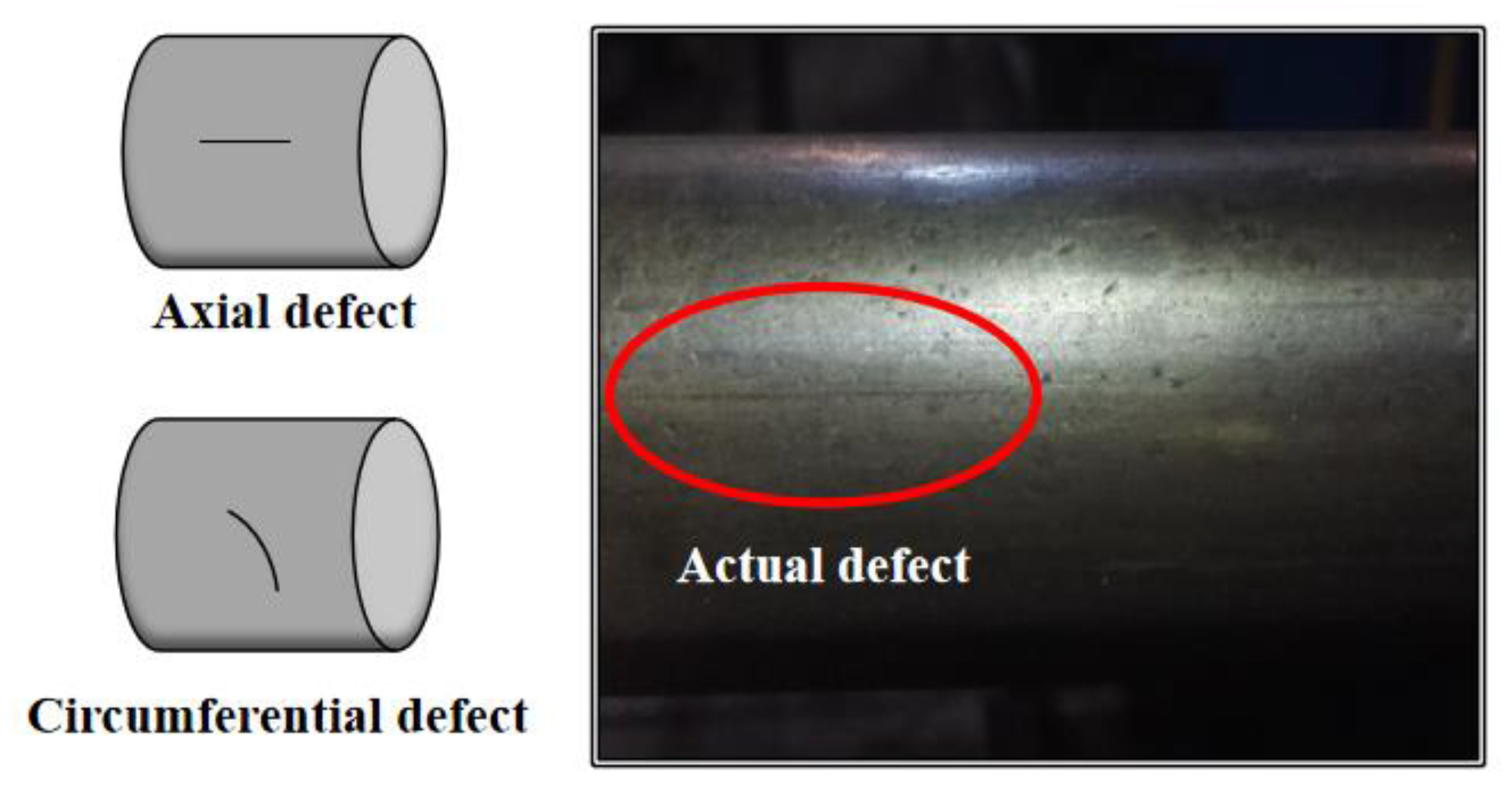
2.1. Grinding Robot Process Introduction
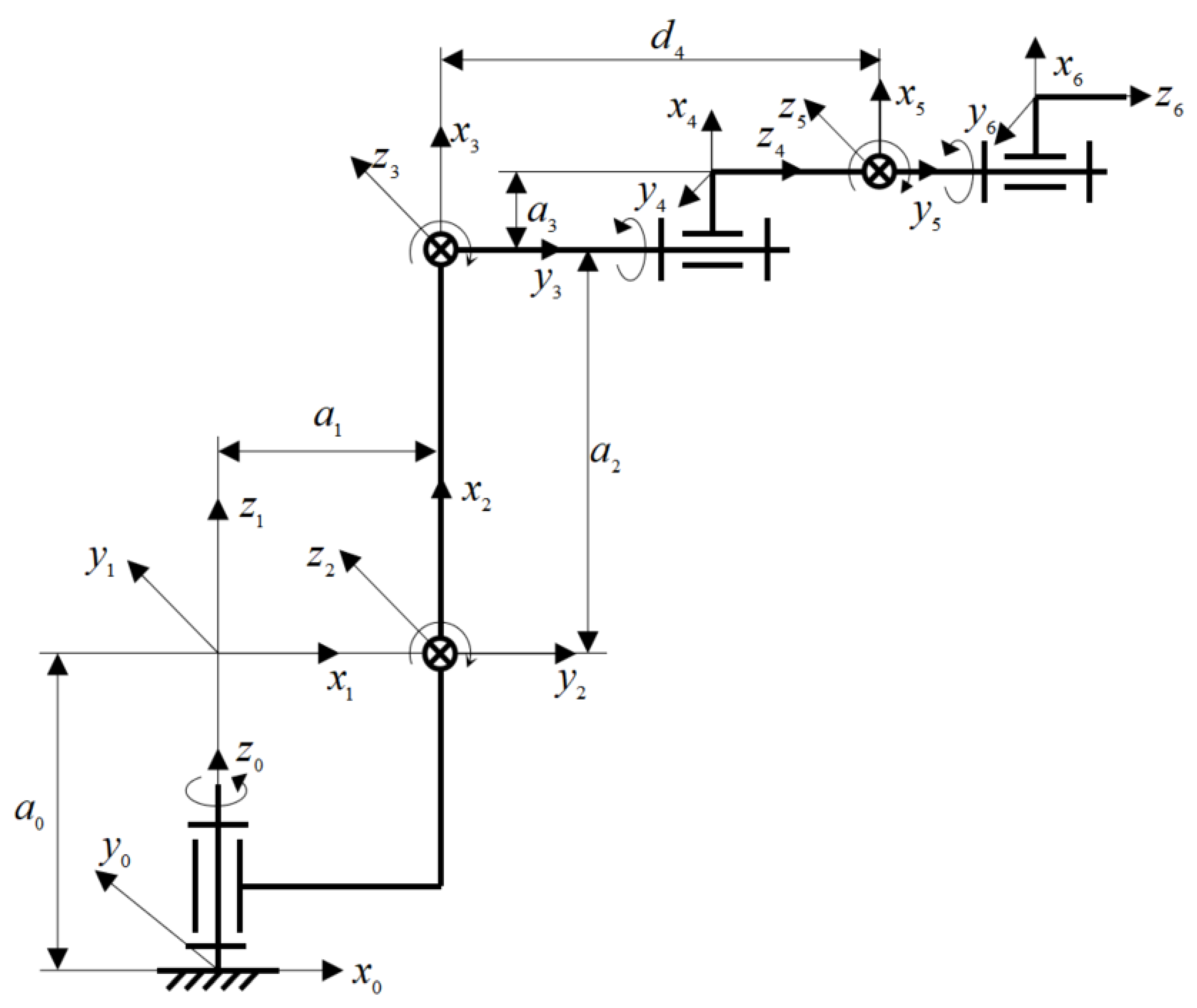
2.2. Grinding Robot Kinematics Model
3. DNN Based Grinding Robot Kinematics Solution
3.1. DNN Overview
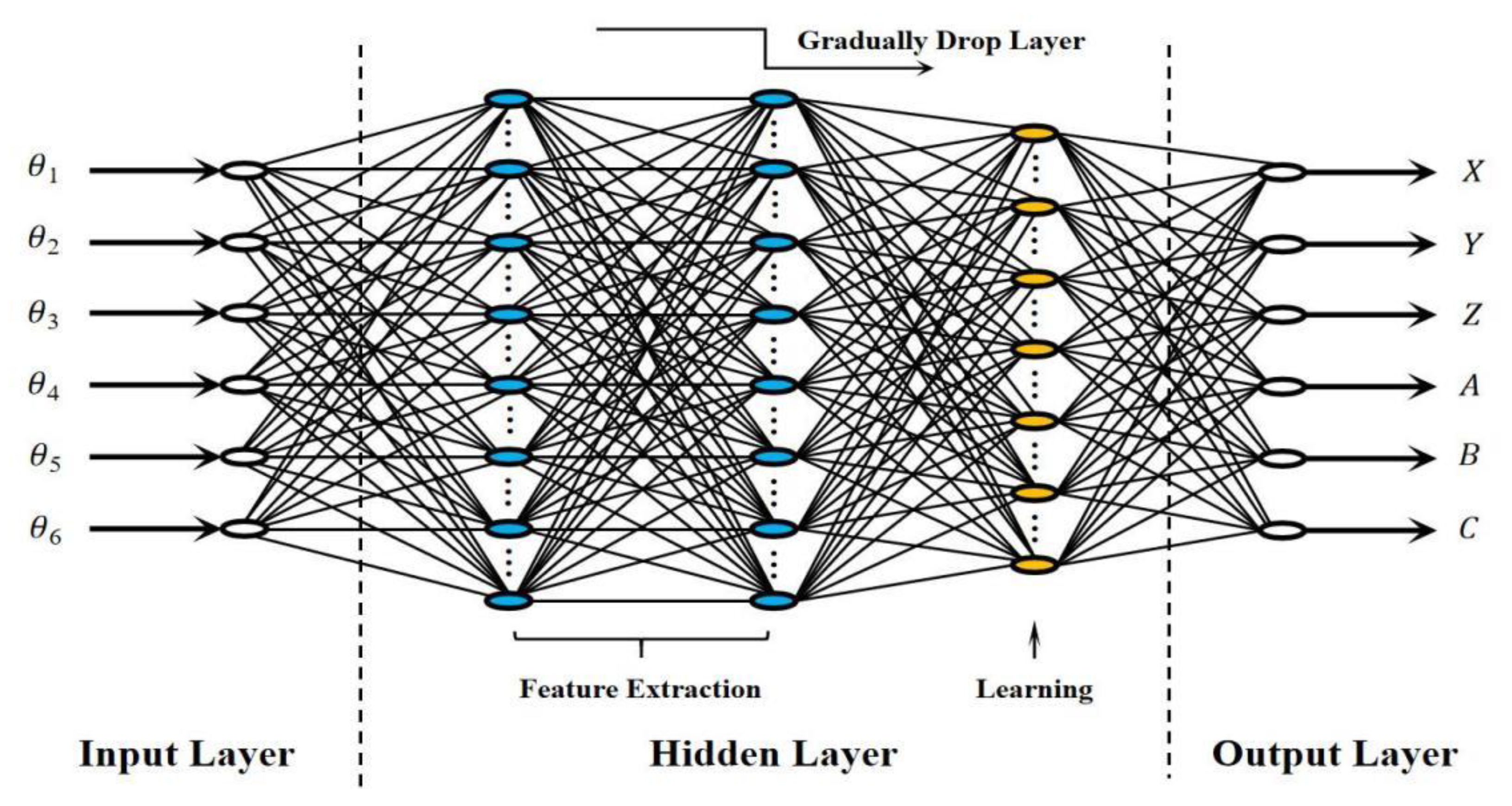
3.2. DNN Model
3.3. Complexity
- (1)
- Forward kinematics solution
- (2)
- Inverse kinematics solution
4. Simulation Experiments and Optimization
4.1. Experimental Scheme
4.2. Simulation Experiments
- (1)
- Conventional stochastic gradient optimization is solved by using an activation function combining stochastic gradient descent (SGD) and hyperbolic tangent (tanh). The curves of the Sigmoid function and tanh function are shown in Figure 8. The advantage is that it is smooth and easy to derivate and can map a real number to the interval [0, 1]. The disadvantage is that the exponential operation has a large amount of calculation, slow descent speed, and there is division in the derivation when the backpropagation is solving the error gradient. In the process of backpropagation, saturated neurons will lead to the disappearance of the gradient, so that the training of the deep network cannot be completed. The fitting situation of SGD plus tanh solution is shown in Figure 9 and Figure 10.
- (2)
- The activation function combining Nesterov adaptive moment estimation (Nadam) and hyperbolic tangent (tanh) is used to complete the experiment. Nadam has a stronger constraint on the learning rate and a more direct influence on the gradient update. In this case, the gradient disappearance still exists. The main advantage of Nadam over Adam is better performance in the case of disappearing gradients. In general, where you want to use RMSprop or Adaptive Moment Estimation (Adam), most can use Nadam for better results. The fitting situation of the Nadam plus tanh solution is shown in Figure 11 and Figure 12.
- (3)
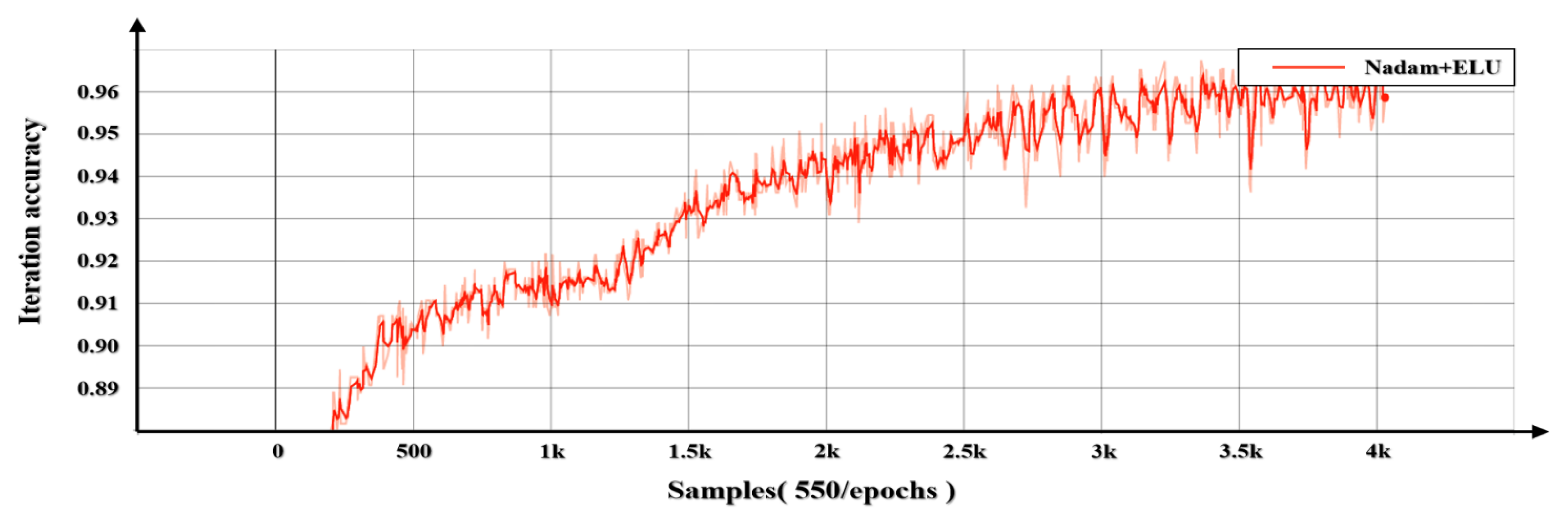
- The activation function combining Nesterov adaptive moment estimation (Nadam) and improved ReLU function (ELU) is used to complete the experiment. The curve of the ELU function is shown in Figure 13. Compared with the ReLU function, there is a certain number of outputs in the case of negative input, and this part of the output has a certain anti-interference ability, which can eliminate the problem of ReLU dying. However, there are still problems with gradient saturation and exponential operation, and the calculation intensity is high. The fitting situation of the Nadam plus ELU solution is shown in Figure 14 and Figure 15.
4.3. Nadam Optimization
- (1)
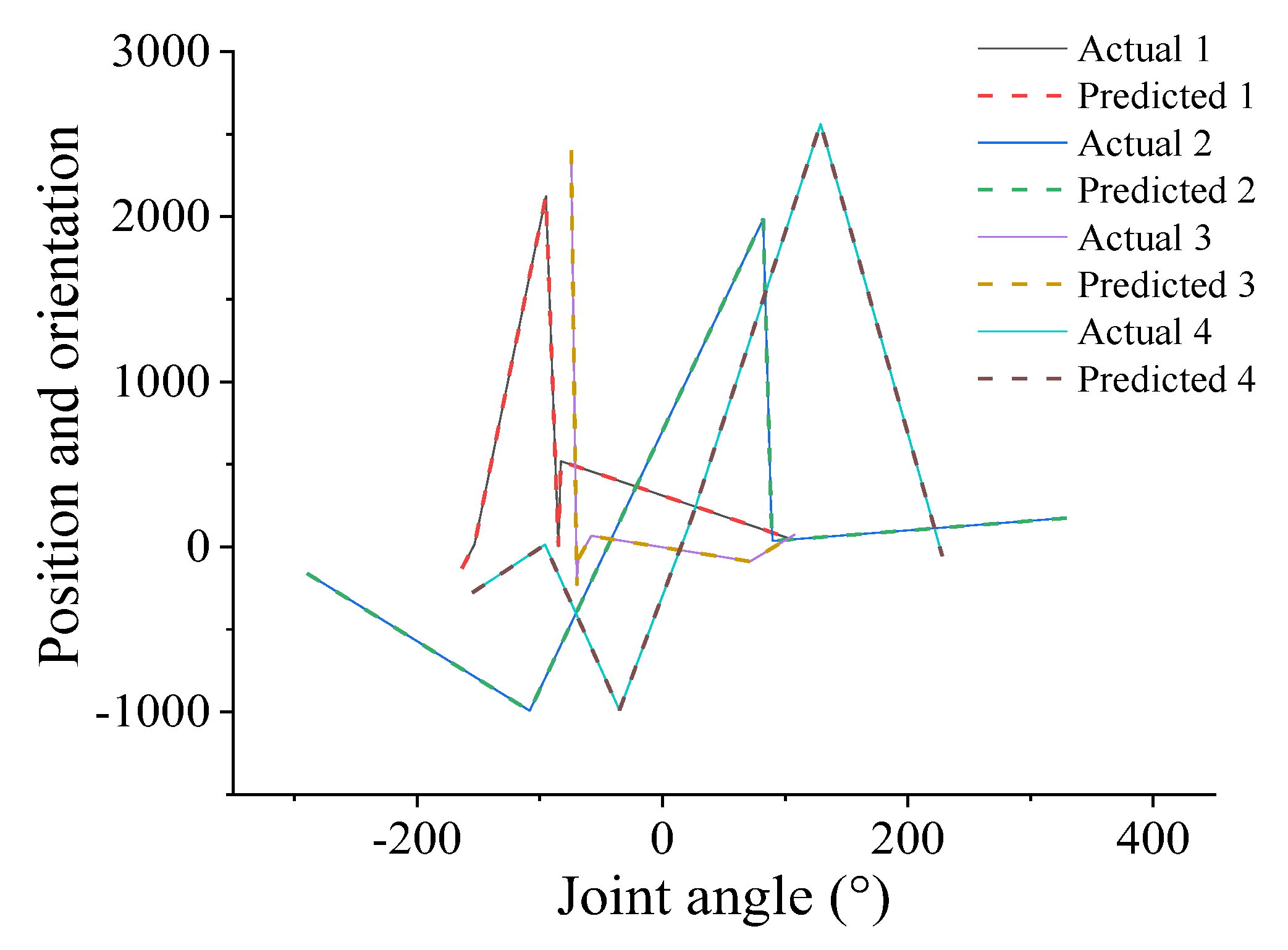
- The relationship between joint angle and terminal position and orientation can be understood as nonlinear regression of and , the nonlinear fitting is carried out by the full connection of layer to layer of DNN, represented as . After running the program, the predicted result of terminal position and orientation can be obtained, and then compared with the theoretical analytical value, the absolute mean error of orientation forward kinematics solution is about 0.02°, the absolute mean error of position forward kinematics solution is about 0.3 mm, they are all within the margin of error. It shows that there is little difference between the predicted value and the analytical solution, which can meet the precision requirement of engineering applications. The comparison curves between the analytic solution and the predicted solution of forward kinematics are shown in Figure 17, the selected sample data is shown in Table 8.
- (2)
- Similarly, the relationship between terminal position and orientation and joint angle can be understood as nonlinear regression of and . The deep neural network is combined with the inverse kinematics solving program, and the unique inverse kinematics solution of the robot is determined by filtering and limiting conditions. After running the program, the predicted result of joint angle can be obtained and then compared with the theoretical analytical value, the absolute mean error of orientation inverse kinematics solution is about 10−5, and it is almost close to 0. It shows that there is little difference between the predicted value and the analytical solution (negligible), which can meet the precision requirement of engineering applications. The comparison curves between the analytic solution and the predicted solution of inverse kinematics are shown in Figure 18, the selected sample data is shown in Table 9.
5. Conclusions
Author Contributions
Funding
Institutional Review Board Statement
Informed Consent Statement
Data Availability Statement
Acknowledgments
Conflicts of Interest
References
- Woodside, M.R.; Fischer, J.; Bazzoli, P.; Bristow, D.A.; Landers, R.G. A kinematic error controller for real-time kinematic error correction of industrial robots. Procedia Manuf. 2021, 53, 705–715. [Google Scholar] [CrossRef]
- Nubert, J.; Koehler, J.; Berenz, V.; Allgower, F.; Trimpe, S. Safe and fast tracking on a robot manipulator: Robust MPC and Neural Network Control. IEEE Robot. Autom. Lett. 2020, 5, 3050–3057. [Google Scholar] [CrossRef] [Green Version]
- Pham, D.T.; Nguyen, T.V.; Le, H.X.; Nguyen, L.; Thai, N.H.; Phan, T.A.; Pham, H.T.; Duong, A.H. Adaptive neural network based dynamic surface control for uncertain dual arm robots. Int. J. Dyn. Control 2020, 8, 824–834. [Google Scholar] [CrossRef] [Green Version]
- Huang, P.; Huang, H.Z.; Li, Y.F.; Li, H. Positioning accuracy reliability analysis of industrial robots based on differential kinematics and saddlepoint approximation. Mech. Mach. Theory 2021, 162, 104367. [Google Scholar] [CrossRef]
- Agbaraji, C.E.; Udeani, U.H.; Inyiama, H.C.; Okezie, C.C. Robust control for a 3-DOF articulated robotic manipulator joint torque under uncertainties. J. Eng. Res. Rep. 2020, 9, 53565. [Google Scholar]
- Le, Q.D.; Kang, H.J. Implementation of fault-tolerant control for a robot manipulator based on synchronous sliding mode control. Appl. Sci. 2020, 10, 2534. [Google Scholar] [CrossRef] [Green Version]
- Liu, W.W. Research on Simulation and Experiment of 6-DOF Industrial Robot’s Dynamic Characteristics. Master’s Thesis, Northeastern University, Boston, MA, USA, 2014. [Google Scholar]
- Xiong, Y.L.; Li, W.L.; Chen, W.B.; Yang, H.; Ding, Y.; Zhao, H. Robotics: Modeling Control and Vision; Huazhong University of Science & Technology Press: Huazhong, China, 2018. [Google Scholar]
- Xie, Z.J.; Feng, C.; Wang, C.F. Kinematics positive solution of 6-PSS parallel robot based on BP neural network. J. Mach. Des. 2014, 31, 36–39. [Google Scholar]
- Li, J.R.; Qi, L.Q.; Han, W.B. Kinematics Analysis and Trajectory Optimization of Six Degree of Freedom Manipulator. J. Chang. Univ. Sci. Technol. 2019, 42, 68–73. [Google Scholar]
- Zhang, H.T. Trajectory simulation control of 6-DOF manipulator based on neural network. Intern. Combust. Engine Parts 2020, 21, 201–202. [Google Scholar]
- Xie, H.; Wang, L.C.; Yuan, X.F.; Chen, H.B. Sliding mode convolutional neural network trajectory tracking control for robot manipulators. Comput. Eng. Appl. 2021, 1–7. [Google Scholar]
- Li, M.W.; Qu, G.Y.; Wei, D.Z.; Jia, H.P. Performance optimization of neural network convolution based on GPU platform. J. Comput. Res. Dev. 2021, 1–10. [Google Scholar]
- Li, H.; Yan, M.Y.; Lv, Z.Y.; Li, W.M.; Ye, X.C.; Fan, D.R.; Tang, Z.M. Survey on graph neural network acceleration arthitecctures. J. Comput. Res. Dev. 2021, 58, 1204–1229. [Google Scholar]
- Xiao, L.; Jia, L.; Dai, J.; Tan, Z. Design and application of a robust zeroing neural network to kinematical resolution of redundant manipulators under various external disturbances. Neurocomputing 2020, 415, 174–183. [Google Scholar] [CrossRef]
- Xu, Z.; Li, S.; Zhou, X.; Yan, W.; Cheng, T.; Huang, D. Dynamic neural networks based kinematic control for redundant manipulators with model uncertainties. Neurocomputing 2019, 329, 255–266. [Google Scholar] [CrossRef]
- Stefan, G.; Hubert, G.; Andreas, M.; Ronald, N. Robot calibration combining kinematic model and neural network for enhanced positioning and orientation accuracy. IFAC Pap. 2020, 53, 8432–8437. [Google Scholar]
- Alebooyeh, M.; Urbanic, R.J. Neural network model for identifying workspace, forward and inverse kinematics of the 7-DOF YuMi 14000 ABB collaborative robot. IFAC Pap. 2019, 52, 176–181. [Google Scholar] [CrossRef]
- Zubizarreta, A.; Larrea, M.; Irigoyen, E.; Cabanes, I.; Portillo, E. Real time direct kinematic problem computation of the 3PRS robot using neural networks. Neurocomputing 2017, 271, 104–114. [Google Scholar] [CrossRef]
- Cursi, F.; Modugno, V.; Lanari, L.; Oriolo, G.; Kormushev, P. Bayesian neural network modeling and hierarchical MPC for a tendon-driven surgical robot with uncertainty minimization. IEEE Robot. Autom. Lett. 2021, 6, 2642–2649. [Google Scholar] [CrossRef]
- Cursi, F.; Chappell, D.; Kormushev, P. Augmenting loss functions of feedforward neural networks with differential relationships for robot kinematic modelling. In Proceedings of the 20th International Conference on Advanced Robotics (ICAR), Ljubljana, Slovenia, 6–10 December 2021; pp. 201–207. [Google Scholar]
- Cursi, F.; Bai, W.; Li, W.; Yeatman, E.M.; Kormushev, P. Augmented neural network for full robot kinematic modelling in SE(3). IEEE Robot. Autom. Lett. 2022, 7, 7140–7147. [Google Scholar] [CrossRef]
- Cronin, N.J. Using deep neural networks for kinematic analysis: Challenges and opportunities. J. Biomech. 2021, 123, 110460. [Google Scholar] [CrossRef]
- Zhao, L.; Jin, J.; Gong, J. Robust zeroing neural network for fixed-time kinematic control of wheeled mobile robot in noise-polluted environment. Math. Comput. Simul. 2021, 185, 289–307. [Google Scholar] [CrossRef]
- Long, C.; Zhang, G.; Zeng, Z.; Hu, J. Finite-time stabilization of complex-valued neural networks with proportional delays and inertial terms: A non-separation approach. Neural Netw. 2022, 148, 86–95. [Google Scholar] [CrossRef] [PubMed]
- Tang, S.; Zhu, Y.; Yuan, S. A novel adaptive convolutional neural network for fault diagnosis of hydraulic piston pump with acoustic images. Adv. Eng. Inform. 2022, 52, 101554. [Google Scholar] [CrossRef]
- Zhu, Q.D.; Wang, X.L. Inverse kinematics algorithm of 6-DOF manipulator. Robot Tech. Appl. 2014, 2, 12–18. [Google Scholar]
- Zhou, X.C.; Meng, Z.D. Algorithm for KUKA robot kinematics calculation. Ind. Control Comput. 2014, 27, 95–97+100. [Google Scholar]
- Zhou, H.; Qin, Y.L.; Chen, H.; Ge, S.Y.; Cao, Y. Structural synthesis of five-degree-of- freedom hybrid kinematics mechanism. J. Eng. Des. 2016, 27, 390–412. [Google Scholar] [CrossRef]
- Sze, V.; Chen, Y.H.; Yang, T.J.; Emer, J.S. Efficient processing of deep neural networks: A tutorial and survey. Proc. IEEE 2017, 105, 2295–2329. [Google Scholar] [CrossRef] [Green Version]
- Zhang, H.Y.; Liu, X.W.; Ren, C.; Zhao, B. Forward kinematics control and NURBS trajectory planning for parallel robots. Mach. Des. Manuf. 2021, 4, 282–286+292. [Google Scholar]
- Liu, S.P.; Cao, J.F.; Sun, T.; Hu, J.B.; Fu, Y.; Zhang, S.; Li, S.J. Inverse kinematics analysis of redundant manipulators based on BP neural network. China Mech. Eng. 2019, 30, 2974–2977+2985. [Google Scholar]
- Jin, F. Fundamental Principles and Methods of Neural Computational Intelligence; Southwest Jiaotong University: Chengdu, China, 2000. [Google Scholar]
- Chen, Y.Y.; Zhang, B.; Fu, Y.X.; Fu, W.; Shen, C.J. Design and kinematics analysis of jujube pruning manipulator. J. Agric. Mech. Res. 2021, 43, 7–11. [Google Scholar]
- Dozat, T. Incorporating nesterov momentum into adam. In Proceedings of the ICLR (2)—Workshop Track, San Juan, Puerto Rico, 24 May 2016. [Google Scholar]
- Sutskever, I.; Marten, J.; Dah, G.E.; Hinton, G.E. On the importance of initialization and momentum in deep learning. In Proceedings of the 30th International Conference on Machine Learning (ICML), Atlanta, GA, USA, 16–21 June 2013; pp. 1139–1147. [Google Scholar]
- Degrave, J.; Felici, F.; Buchli, J.; Neunert, M.; Tracey, B.; Carpanese, F.; Ewalds, T.; Hafner, R.; Abdolmaleki, A.; Casas, D.D.L.; et al. Magnetic control of tokamak plasmas through deep reinforcement learning. Nature 2022, 602, 414–419. [Google Scholar] [CrossRef] [PubMed]


| i | ai−1 | αi−1 | di | θi | θi Scope |
|---|---|---|---|---|---|
| 1 | 0 | 0 | 0 | θ1 | +/−185° |
| 2 | a1 | −90° | 0 | θ2 | −5~−140° |
| 3 | a2 | 0 | 0 | θ3 | +155~−120° |
| 4 | a3 | −90° | d4 | θ4 | +/−350° |
| 5 | 0 | 90° | 0 | θ5 | +/−122.5° |
| 6 | 0 | −90° | 0 | θ6 | +/−350° |
| i | Layer | Input Dimension n | Element Dimension d | Neuron x | Time Complexity | Space Complexity |
|---|---|---|---|---|---|---|
| 1 | Fully Connected | 6 | 1 | 64 | O (n * d * x) | S (n * d * x) |
| 2 | Activation | 64 | 1 | N/A | O (n * d) | S (n) |
| 3 | Fully Connected | 64 | 1 | 64 | O (n * d * x) | S (n * d * x) |
| 4 | Activation | 64 | 1 | N/A | O (n * d) | S (n) |
| 5 | Fully Connected | 64 | 1 | 64 | O (n * d * x) | S (n * d * x) |
| 6 | Activation | 64 | 1 | N/A | O (n * d) | S (n) |
| 7 | Fully Connected | 64 | 1 | 32 | O (n * d * x) | S (n * d * x) |
| 8 | Activation | 32 | 1 | N/A | O (n * d) | S (n) |
| 9 | Fully Connected | 32 | 1 | 16 | O (n * d * x) | S (n * d * x) |
| 10 | Activation | 16 | 1 | N/A | O (n * d) | S (n) |
| 11 | Fully Connected | 16 | 1 | 6 | O (n * d * x) | S (n * d * x) |
| i | Layer | Input Dimension n | Element Dimension d | Neuron x | Time Complexity | Space Complexity |
|---|---|---|---|---|---|---|
| 1 | Fully Connected | 6 | 1 | 128 | O (n * d * x) | S (n * d * x) |
| 2 | Activation | 128 | 1 | N/A | O (n * d) | S (n) |
| 3 | Fully Connected | 128 | 1 | 128 | O (n * d * x) | S (n * d * x) |
| 4 | Activation | 128 | 1 | N/A | O (n * d) | S (n) |
| 5 | Fully Connected | 128 | 1 | 128 | O (n * d * x) | S (n * d * x) |
| 6 | Activation | 128 | 1 | N/A | O (n * d) | S (n) |
| 7 | Fully Connected | 128 | 1 | 128 | O (n * d * x) | S (n * d * x) |
| 8 | Activation | 128 | 1 | N/A | O (n * d) | S (n) |
| 9 | Fully Connected | 128 | 1 | 128 | O (n * d * x) | S (n * d * x) |
| 10 | Activation | 128 | 1 | N/A | O (n * d) | S (n) |
| 11 | Fully Connected | 128 | 1 | 128 | O (n * d * x) | S (n * d * x) |
| 12 | Activation | 128 | 1 | N/A | O (n * d) | S (n) |
| 13 | Fully Connected | 128 | 1 | 64 | O (n * d * x) | S (n * d * x) |
| 14 | Activation | 64 | 1 | N/A | O (n * d) | S (n) |
| 15 | Fully Connected | 64 | 1 | 32 | O (n * d * x) | S (n * d * x) |
| 16 | Activation | 32 | 1 | N/A | O (n * d) | S (n) |
| 17 | Fully Connected | 32 | 1 | 16 | O (n * d * x) | S (n * d * x) |
| 18 | Activation | 16 | 1 | N/A | O (n * d) | S (n) |
| 19 | Fully Connected | 16 | 1 | 6 | O (n * d * x) | S (n * d * x) |
| i | θ1 | θ2 | θ3 | θ4 | θ5 | θ6 |
|---|---|---|---|---|---|---|
| 1 | 169.152 | −74.474 | 100.077 | −250.680 | −19.168 | 291.015 |
| 2 | 108.117 | −10.469 | 60.329 | −325.002 | 85.537 | 303.795 |
| 3 | 66.132 | −37.705 | 84.361 | −75.441 | 38.092 | −230.169 |
| 4 | 76.237 | −135.703 | −43.846 | −317.680 | −98.703 | 226.420 |
| 5 | −140.971 | −72.721 | 143.930 | −111.730 | 20.891 | −193.332 |
| 6 | −92.969 | −105.562 | 19.138 | 139.354 | 95.771 | 321.504 |
| 7 | 17.470 | −121.286 | −78.944 | −169.744 | 83.476 | −172.002 |
| 8 | 116.285 | −107.124 | 135.547 | −105.011 | −74.334 | −174.241 |
| 9 | 42.937 | −76.106 | −23.294 | 231.580 | 20.890 | 34.807 |
| 10 | 154.362 | −101.412 | 88.230 | 177.610 | −29.291 | 47.475 |
| Method + Iteration | 2000 | 10,000 | 100,000 | 400,000 |
|---|---|---|---|---|
| SGD + Tanh | 80.9% | 80.9% | 80.9% | 80.9% |
| Nadam + Tanh | 87.1% | 88.3% | 88.3% | 88.3% |
| Nadam + ELU | 90.9% | 93.4% | 97.8% | 98.5% |
| Method + Iteration + Consumption Time | SGD + Tanh | Nadam + Tanh | Nadam + ELU |
|---|---|---|---|
| 2000 | 80.9% | 87.1% | 90.9% |
| Single iteration time consumption | 20 ms | 22 ms | 22 ms |
| Total time consumption | 40 s | 45 s | 45 s |
| 10,000 | 80.9% | 88.3% | 93.4% |
| Single iteration time consumption | 20 ms | 22 ms | 22 ms |
| Total time consumption | 3 min 21 s | 3 min 47 s | 3 min 44 s |
| 100,000 | 80.9% | 88.3% | 97.8% |
| Single iteration time consumption | 20 ms | 22 ms | 22 ms |
| Total time consumption | 33 min 16 s | 33 min 51 s | 33 min 57 s |
| 400,000 | 80.9% | 88.3% | 98.5% |
| Single iteration time consumption | 20 ms | 22 ms | 22 ms |
| Total time consumption | 2 h 14 min 26 s | 2 h 27 min 06 s | 2 h 28 min 25 s |
| Method + Accuracy | Time Required for 80% Accuracy | Time Required for 85% Accuracy | Time Required for 90% Accuracy | Time Required for 95% Accuracy |
|---|---|---|---|---|
| SGD + Tanh | About 30 s | N/A | N/A | N/A |
| Nadam + Tanh | About 20 s | About 30 s | N/A | N/A |
| Nadam + ELU | About 20 s | About 30 s | About 45 s | About 10 min |
| 1 | Joint angle actual value | 103.157 | −82.834 | −95.024 | −163.470 | −84.854 | −153.296 |
| Position and orientation actual value | 51.512 | 519.156 | 2124.172 | −130.236 | 4.834 | 16.073 | |
| Position and orientation predicted value | 52.048 | 519.625 | 2124.669 | −130.266 | 4.825 | 16.080 | |
| 2 | Joint angle actual value | 88.812 | −108.298 | 82.113 | 329.419 | 89.898 | −289.636 |
| Position and orientation actual value | 142.725 | −993.218 | 1986.104 | 174.860 | 35.362 | −161.150 | |
| Position and orientation predicted value | 143.089 | −993.617 | 1986.581 | 174.353 | 35.718 | −161.664 | |
| 3 | Joint angle actual value | −69.850 | −68.648 | −74.447 | 71.387 | −58.072 | 107.855369 |
| Position and orientation actual value | −231.802 | −71.347 | 2403.578 | −87.774 | 66.774 | 75.165 | |
| Position and orientation predicted value | −232.019 | −71.836 | 2403.117 | −88.013 | 66.384 | 75.881 | |
| 4 | Joint angle actual value | −155.081 | −35.073 | 128.912 | 23.640 | −95.757 | 228.066 |
| Position and orientation actual value | −278.397 | −988.946 | 2562.402 | 171.416 | 12.991 | −55.852 | |
| Position and orientation predicted value | −278.662 | −989.034 | 2562.831 | 171.956 | 12.448 | −55.725 |
| 1 | Position and orientation actual value | 1131.414 | −7.778 | 124.19 | −11.456 | −55.673 | −93.113 |
| Joint angle actual value | 12.630900 | −20.476474 | 127.226347 | 88.156338 | −88.722097 | −197.538884 | |
| Joint angle predicted value | 12.630894 | −20.476461 | 127.226353 | 88.156347 | −88.722106 | −197.538896 | |
| 2 | Position and orientation actual value | 835.82 | −16.01 | 614.392 | −47.505 | −11.666 | −170.864 |
| Joint angle actual value | 0.474678 | −81.717642 | 154.329096 | 218.121807 | −3.515341 | 276.113429 | |
| Joint angle predicted value | 0.474703 | −81.717651 | 154.329104 | 218.121796 | −3.515348 | 276.113437 | |
| 3 | Position and orientation actual value | −380.804 | −2003.691 | 815.821 | −76.990 | −10.079 | −87.533 |
| Joint angle actual value | 106.601969 | −34.660064 | 63.840859 | −256.547298 | −117.218808 | 41.888494 | |
| Joint angle predicted value | 106.602017 | −34.660035 | 63.840873 | −256.547304 | −117.218824 | 41.888486 | |
| 4 | Position and orientation actual value | −1613.768 | −765.244 | 2298.126 | 48.712 | 20.206 | −90.383 |
| Joint angle actual value | 147.210303 | −59.896149 | 18.556023 | 78.966712 | 78.258449 | 22.322419 | |
| Joint angle predicted value | 147.210309 | −59.896154 | 18.556041 | 78.966708 | 78.258453 | 22.322422 |
Disclaimer/Publisher’s Note: The statements, opinions and data contained in all publications are solely those of the individual author(s) and contributor(s) and not of MDPI and/or the editor(s). MDPI and/or the editor(s) disclaim responsibility for any injury to people or property resulting from any ideas, methods, instructions or products referred to in the content. |
© 2023 by the authors. Licensee MDPI, Basel, Switzerland. This article is an open access article distributed under the terms and conditions of the Creative Commons Attribution (CC BY) license (https://creativecommons.org/licenses/by/4.0/).
Share and Cite
Shi, W.; Zhang, J.; Li, L.; Li, Z.; Zhang, Y.; Xiong, X.; Wang, T.; Huang, Q. Analysis of Efficient and Fast Prediction Method for the Kinematics Solution of the Steel Bar Grinding Robot. Appl. Sci. 2023, 13, 1212. https://doi.org/10.3390/app13021212
Shi W, Zhang J, Li L, Li Z, Zhang Y, Xiong X, Wang T, Huang Q. Analysis of Efficient and Fast Prediction Method for the Kinematics Solution of the Steel Bar Grinding Robot. Applied Sciences. 2023; 13(2):1212. https://doi.org/10.3390/app13021212
Chicago/Turabian StyleShi, Wei, Jinzhu Zhang, Lina Li, Ziliang Li, Yanjie Zhang, Xiaoyan Xiong, Tao Wang, and Qingxue Huang. 2023. "Analysis of Efficient and Fast Prediction Method for the Kinematics Solution of the Steel Bar Grinding Robot" Applied Sciences 13, no. 2: 1212. https://doi.org/10.3390/app13021212