Investigating the Effects of Cell Size in Statistical Landslide Susceptibility Modelling for Different Landslide Typologies: A Test in Central–Northern Sicily

Abstract

Optimally sizing grid cells is a relevant research issue in landslide susceptibility evaluation. In fact, the size of the adopted mapping units influences several aspects spanning from statistical (the number of positive/negative cases and prevalence and resolution/precision trade-off) and purely geomorphological (the representativeness of the mapping units and the diagnostic areas) to cartographic (the suitability of the obtained prediction images for the final users) topics. In this paper, the results of landslide susceptibility modelling in a 343 km² catchment for three different types of landslides (rotational/translational slides, slope flows and local flows) using different pixel-size mapping units (5, 8, 10, 16 and 32 m) are compared and discussed. The obtained results show that the higher-resolution model (5 m) did not produce the best performance for any of the landslide typologies. The model with 8 m sized pixels displayed the optimal threshold size for slides and slope flows. In contrast, for local flows, an increasing trend of model prediction accuracy was reached with 32 m pixels, which was a higher value than that presented using 8 m pixels. The variable importance analysis demonstrated that the better performance of the 8 m cells was due to their effectiveness in capturing morphological conditions which favour slope instability (profile curvature and middle and high ridges).

1. Introduction

Landslide susceptibility (LS) statistical modelling requires study areas to be partitioned into a set of mapping units where, based on the matching between predictors (the controlling factors) and outcome (the stable/unstable slope status), the main dataframes required for regression or classification are extracted. Among the different mapping units which can be adopted in LS modelling (e.g., grid cells, slope units and terrain units), square grid cells are largely exploited as they directly replicate the data structure of digital terrain models (DTMs), which constitute the main source layer for the derivation of those covariates, which potentially explain the spatial distribution of landslides (the controlling factors). At the same time, grid cells furnish an objective criterion in choosing the operative mapping unit in LS mapping. However, potential uncoupling between the grid’s regular geometry and the randomness of the morphodynamic phenomena could arise and hamper the quality of the susceptibility models. In this sense, a key point in adopting grid-based mapping units is the optimal sizing of the cell by assuming one of the source DTMs as a minimum extension. In fact, the size of the adopted grid cells potentially influences the final susceptibility map results that are obtained, either in terms of predictive performance (accuracy and reliability), the geomorphological adequateness of the models or the ease with which maps can be handled by the final users.

Reducing the size of the grid cells can result in an increase in model resolution; however, the accuracy of the final susceptibility map depends on optimal coupling between cell dimension and the controlling factor of spatial variability in the so-called diagnostic areas (where we assume we recognise the conditions for the activation of the known calibration phenomena). In this sense, even for small phenomena, instability conditions are frequently captured in spatial domains larger than a very small pixel. It is worth stressing this point, considering the current availability of centimetric DTMs derived from airborne or drone image/LIDAR acquisition. In addition, typical diagnostic areas in regional or large inventories are simply defined as corresponding to Landslide Identification Points (LIPs), located at the highest point along the crown area of the landslide scarps or source areas, which means we can expect to decipher the causes of slope instability in a single cell hosting at least one point.

This issue has been explored in a number of papers which have addressed different types of landslides. In particular, Palamakumbure et al. [1] focused on the flow type of the Sidney basin by exploiting 2, 5, 10, 15, 20, 25, 30 and 40 m resolutions, concluding that the medium resolutions performed better than the rest. Cama et al. [2] analysed the effect of grid cells’ size on debris flows in the Giampilieri basin (Sicily, Italy), focusing on 2, 4, 16 and 32 m resolutions. Between the high performances obtained for all of the models, the 16 m resolution produced slightly better predictions, while the 32 m resolution showed the worst. Similarly, Arnone et al. [3] investigated the effect of the raster resolution on susceptibility evaluation for debris and mud flows in the Briga and Giampilieri catchments (Sicily, Italy) considering 10, 20, 30, 40 and 50 m DTMs. The best performances were obtained from the medium resolutions, thus concluding that “not always an increase of resolution implies an improvement in the susceptibility analysis”. Shirzadi et al. [4] analysed the effect on shallow landslides (Bijar region, Iran) by considering six different raster resolutions (10, 15, 20, 30, 50 and 100 m). In this case, better performances were obtained by employing the minimum tested size (10 m). Zhao et al. [5] tested three resolutions (5, 15 and 30 m) by employing a mixed inventory of slides, falls and debris flows triggered by a 2013 earthquake in Lushan, China; once again, the best performance was obtained from the medium resolution (15 m). Using a mixed inventory (mainly slides, debris flows and falls) triggered by a 2013 earthquake in Lushan, China, Shao et al. [6] tested the effect of 2.5, 5, 10, 20, 40 and 80 m resolutions in statistical landslide susceptibility evaluation, concluding that “the results show that the satisfactory result could be achieved with high-resolution DTMs but the accuracy of landslide prediction becomes increasingly worse with coarser resolutions”. By contrast, for shallow landslides, Liao et al. [7] tested very coarse resolutions (30, 300, 1000, 2000 and 3000 m), but better performances were obtained from a very low resolution (2000 m).

In this research, a robust inventory including three different types of landslides was exploited to explore the effect of changing the cell size of mapping units on the inner structure of the three derived susceptibility models (i.e., the involved dominant controlling factors) and on their predictive performance (accuracy and reliability). In fact, this analysis of the effects of cell sizing on the model accuracy using the same source data and different slope failure types offered a key to the interpretation of any predictive performance changes, also in light of the geomorphological suitability of the related factor selection.

Other types of landslides were excluded from the analysis (such as falls, topples and deep-seated landslides) due to the fact that, generally, a direct and/or physical-based approach is employed for their susceptibility evaluation (e.g., [8,9,10,11,12,13]).

LS modelling was performed by applying Multiple Adaptive Regression Splines statistical modelling to regress the three-type landslide inventory and a set of controlling factors by using five (5, 8, 10, 16, and 32 m) mapping units.

2. Materials and Methods

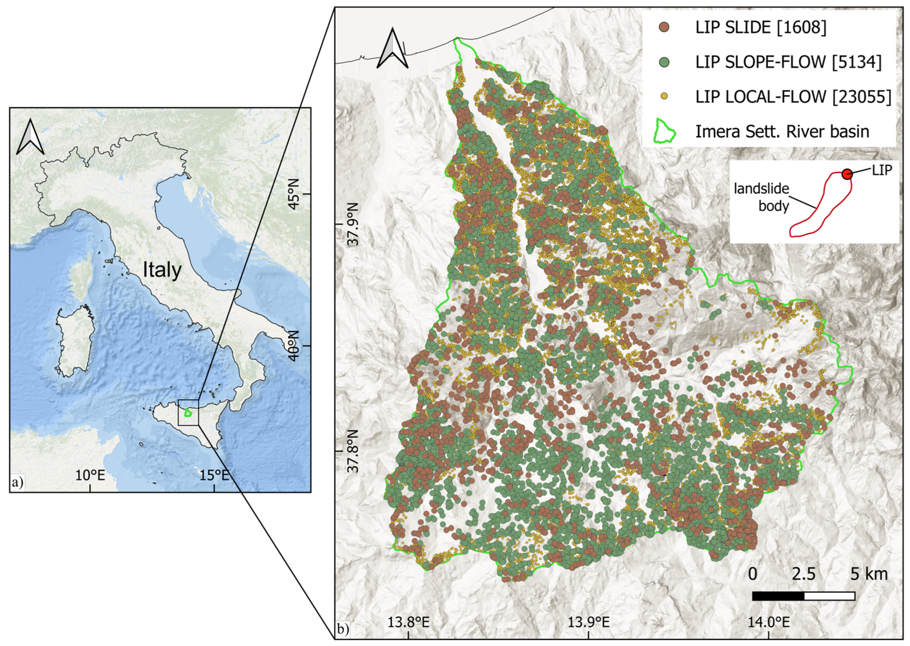
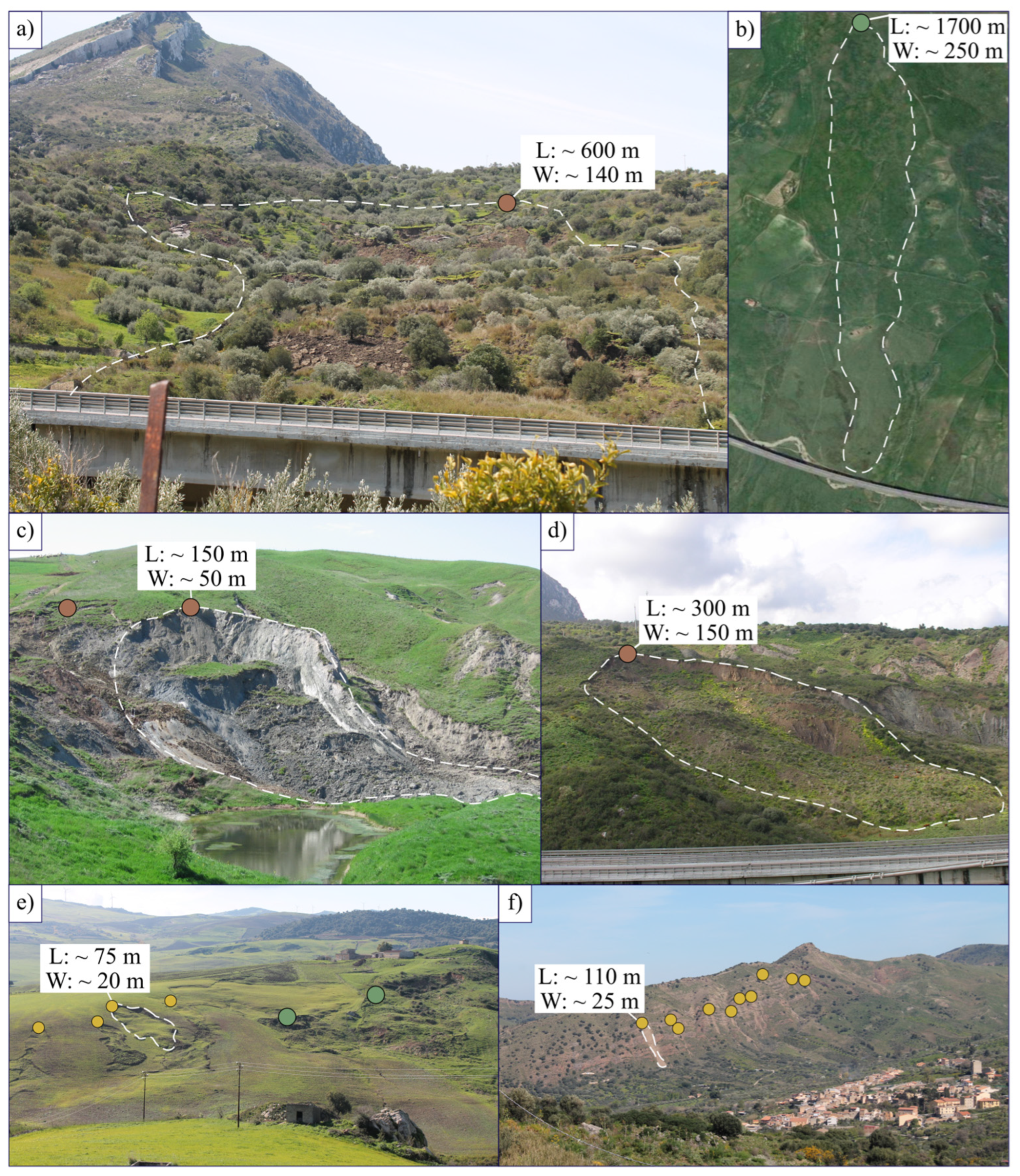
2.1. Study Area and Landslides Inventories

The Imera Settentrionale River basin is 343 km² long in northern Sicily (Italy, Figure 1a), between the northern sector of the Madonie Mountains and the Tyrrhenian Sea. The central–western sector of the Sicilian Fold and Thrust Belt, in which the basin falls, is the result of the retreat of the subduction hinge of the Ionian oceanic lithosphere and the post-collisional convergence between Africa and Europe [14,15,16]. The intense compressive tectonic activity starting in the Oligocene [17] was followed by a syntectonic relaxing phase, during which the thrust sheets’ basins were filled with terrigenous deposits [18]. Due to this tectonic activity, the basin is characterised by a hilly landscape and isolated carbonate reliefs. Rills, gullies, pipes, badlands systems [19,20,21,22,23,24] and landslides [25,26,27,28,29,30] model the slopes where carbonate, siliceous–carbonate and siliciclastic successions alternate with more ductile pelitic flysch sediments, alluvial clastic sediments and marine pelite outcrops [29,30].

As statistical models are calibrated on landslide sets for which common factors are expected to control the potential instability conditions, a susceptibility-analysis-oriented re-classification scheme was proposed here. In particular, three types of landslides are defined in the landslide inventory (Figure 1b): “slides”, “slope flows” and “local flows”.

In particular, rotational and translational slides (1608 cases—Figure 2a,c,d) are grouped together as we assumed to be explainable by recalling the role of the same predictors. In fact, they are strongly controlled by the type of outcropping lithology, being typically generated from alternances of pelitic and arenitic layers. In fact, the arenitic caprock allows for the maintenance of steep slopes and for the required infiltration downward to the pelitic (silty to sandy clays) levels, feeding the failure surfaces. At the same time, in this research, small (local) and large multi-storied (slope) flow landslides were split into two classes. Slope flows (5134 cases—Figure 2b,e) are typical in the Sicilian Apennines and correspond to very large, non-rapid earth/debris flows, frequently involving those slopes totally set on pelitic units. Both slides and slope flows are characterised by large extensions and diachronic activity. In the susceptibility analysis, LIPs were extracted along the crown boundary at its highest topographic point. In contrast, local flows (23,055 cases—Figure 2e,f) are small, non-rapid earth flows and densely affect the pelitic slopes, with a very limited extension of the total landslide area. In addition, these surficial slope failures almost seasonally activate, accounting for a wandering-like spatial distribution inside the clayey slopes. In light of their limited extension and ephemeral features, they were directly mapped with a LIP alone.

To correctly define the date of the activation of phenomena (and to potentially link the landslide inventory with a singular rainfall season), the landslide inventories were detected using high-resolution (0.25 m) LIDAR (Light Detection and Ranging) images taken in 2012 by ARTA (Assessorato Regionale al Territorio e all’Ambiente) and compared with four different Google Earth satellite images dated 15 July 2011 (DigitalGlobe Catalog ID: 1030050011F8C200), 29 June 2011 (DigitalGlobe Catalog ID: 103001000B21B700), 21 June 2011 (DigitalGlobe Catalog ID: 103001000B544500) and 3 May 2013 (DigitalGlobe Catalog ID: 103001002332DE00).

LIPs, assumed to be diagnostic in potentially marking unstable slope conditions [31,32,33,34,35,36,37], were exploited as diagnostic areas.

2.2. Mapping Units and Geo-Environmental Predictors

According to the aim of the research, starting with high-resolution (0.25 m) LIDAR (Light Detection and Ranging) images taken in 2012 by ARTA (Assessorato Regionale al Territorio e all’Ambiente), five grid cells of different resolutions (5, 8, 10, 16 and 32 m) were adopted as mapping units. By overlapping the grid cells with the landslide inventories, the unstable status of each pixel was then assigned with respect to each landslide type investigated, depending on whether it hosted at least one LIP.

Based on the expected influence of geo-environmental variables in landsliding and according to the literature (e.g., [29,30,38,39,40]), 10 variables were exploited as potential predictors for landslide susceptibility modelling.

Elevation (ELE) is considered a proxy of the mean annual which typically reflects the altitude [29]; steepness (SLO) is linked to the inclination of potential underlying rupture surfaces, and it controls the speed of water [29,38]; aspects, expressed here in terms of northernness (N) and easternness (E), can be used to determine the seasonal wet/dry cycles of soils [40]; topographic curvatures, expressed in terms of plan (PLC) and profile curvature (PRF), are assumed to express the direction of flow and shallow mechanical stresses [29,38,41]; the topographic wetness index (TWI) is a good proxy for estimating the potential infiltration [31] or saturated soil thickness; the stream power index (SPI) expresses the intensity of surface water erosion [29,42]; landform classification (LCL) directly differentiates the morphological setting of the study area [29]; the outcropping lithology (LITO) is assumed to be a good proxy for the physical–mechanical properties of rocks at the basin scale [29]; finally, soil use, obtained here via CORINE 2018, is directly related to the potential hydrological and surface water disturbances induced by erosion [29,42].

All the DTM-derived variables passed the test for multicollinearity.

2.3. Statistical Model, Validation Tools and Model-Building Strategies

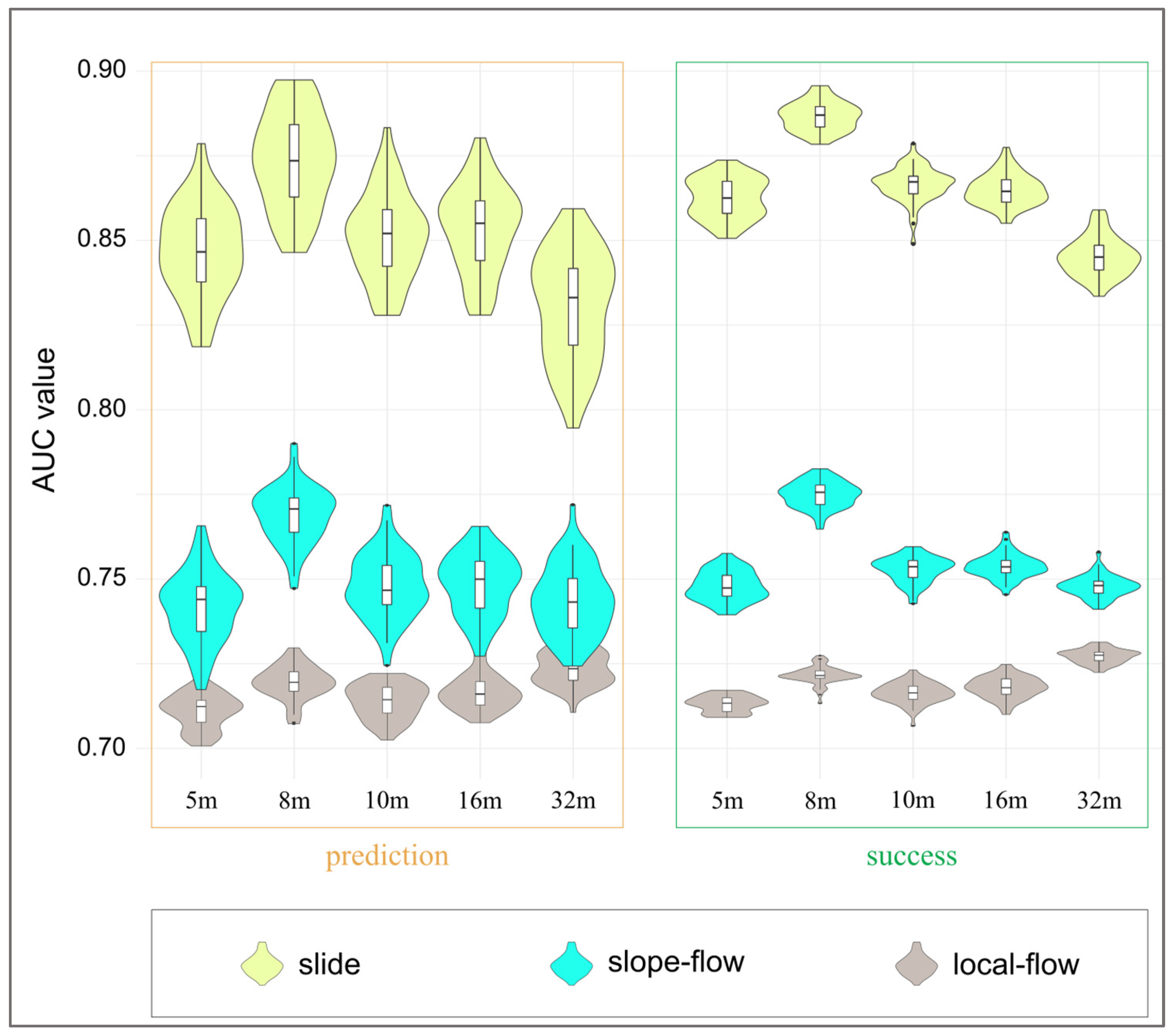
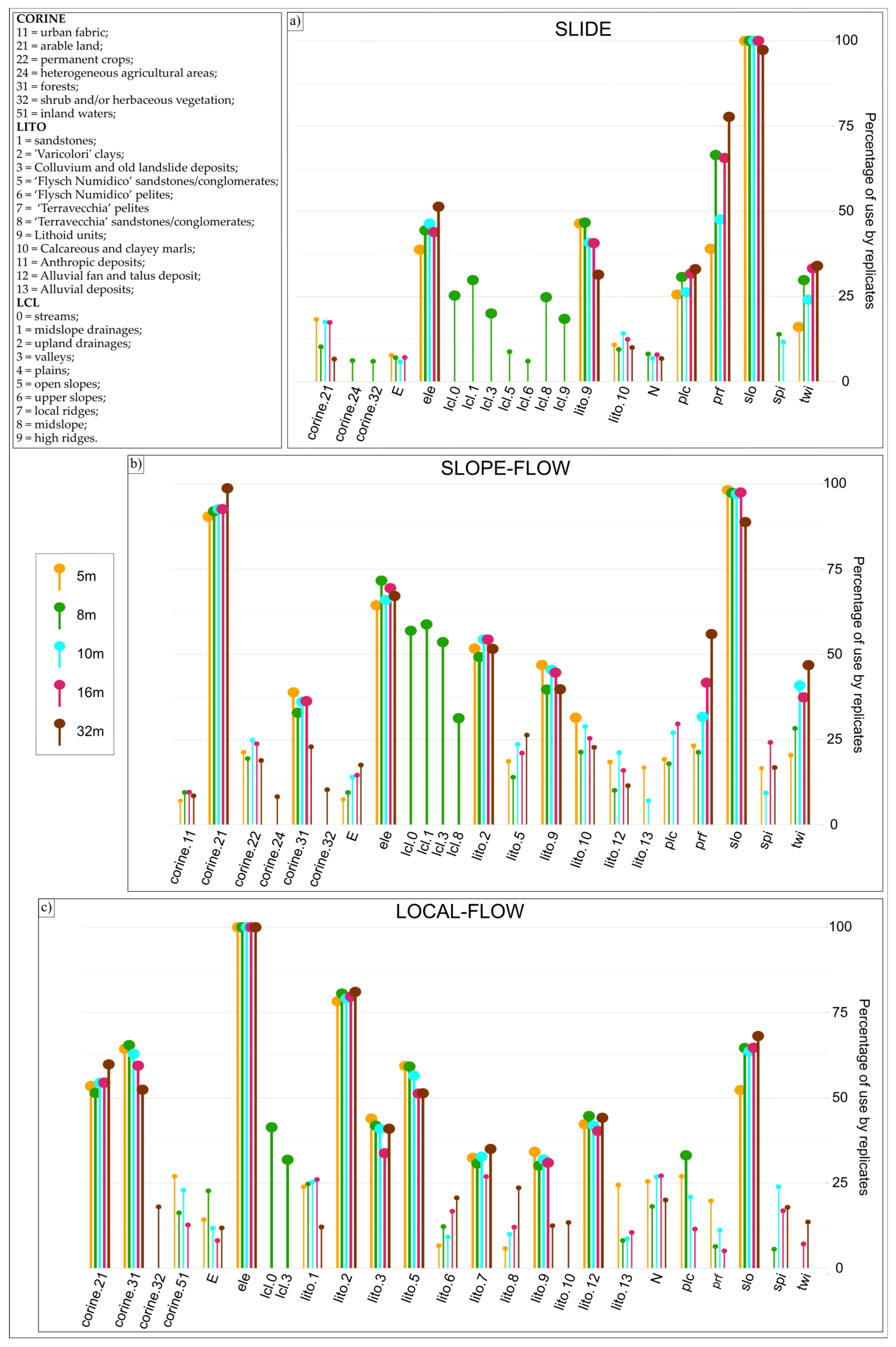
The Multivariate Adaptive Regression Splines (MARS; [43]) method was employed to detect the relations between the outcome and predictors. MARS is based on non-parametric regression, which exploits the splitting of each independent variable into hinge functions to boost the maximum-likelihood-based adaptation skill of the logistic regression method, according to

$$y=f\left(x\right)=\mathsf{\alpha }+{\displaystyle \sum }_{i=1}^N{\beta }_i{h}_i\left(x\right)$$

(1)

where y is the dependent variable (the outcome) predicted by the function f(x), α is the model intercept, and β_i is the coefficient of the h_i basis functions, given the N number of basis functions.

The MARS method is largely employed in several fields of science (e.g., [44,45]), but in the last ten years, MARS has been successfully employed in landslide susceptibility evaluation (e.g., [29,30,36,40,42,46,47,48,49,50]). In this research, MARS analysis was performed by exploiting the “earth” R-package [51]. Based on previous MARS applications [26,29,30,37,42,50], in order to avoid overfitted models and obtain results with geomorphological adequacy in terms of evaluation, we accepted the default setting of the “earth” R-package (see [51] for details), limiting the number of terms in the range of 20–200 and setting it with no interaction.

The MARS method is based on a presence–absence approach. For this reason, the random extraction of the same number of negative and positive cases was carried out. To test the independence of the results (resolution, precision and robustness) from the choice of the selected cases [29,30,42], the extraction of the balanced datasets was repeated fifty times. Moreover, a balanced random partition of each dataset into calibration (75%) and validation (25%) subsets was replicated one hundred times. The prediction skill and the reliability of the models was estimated on the base of five thousand validation tests.

According to Hosmer and Lemeshow [52], the AUC value (Area under Curve) in the ROC (Receiver Operating Characteristics [53,54,55]) was employed to evaluate the prediction skill of the model. At the same time, the Youden index optimised score cut-off [56] was obtained from the ROC plots. In this way, True Positive (TP), True Negative (TN), False Positive (FP) and False Negative (FN) cases were defined, and the related cut-off-dependent indices were calculated. For the balanced analysed datasets, the sensitivity (TPrate) is equal to the ratio of TP/positive cases and 1-FN; the specificity (TNrate) is equal to the ratio of TN/negative cases and 1-FP; the accuracy was equal to the ratio of True/False rate.

In this research, using five different cell sizes (5, 8, 10, 16 and 32 m) and three types of landslides, a set of 15 models was evaluated. For each model, the prediction skill in evaluating the blinded 25% (prediction), and 100% (success) of the archive was analysed by exploiting all of the validation indices/instruments (ROC plot, AUC value and confusion matrix). On the other hand, an in-depth comparison of the employed geo-environmental variables (or classes) for the construction of the 15 models was carried out. In fact, using the “varImp” function of the Caret R-package [57], the percentage of use of each variable by the replicates was calculated.

3. Results

In Figure 3, the violin plots of the AUC values obtained by the replicates for each model group (related to the mapping unit size) are reported. For each group, the variability of the models’ AUC values is represented by the length of each violin, while the width reflects the number of replicates showing the specific value.

The comparison of the performances of the models for the three landslide typologies, obtained for the varying cell size suite, confirmed the expected influence of the mapping units’ size on the accuracy of the models. The AUC values for slide and slope flows were marked by a maximum value for the 8 m cell size and a minimum for 32 m, with differences of about 0.03. The 8 m models approached outstanding—for slide—and excellent—for slope flows—AUC levels. In general, the results regarding local flows showed poorer performances, but a linear positive trend was clearly shown in the AUC values with increasing cell size, up to a largely satisfactory response for 32 m. In addition, generally, the local-flow models were characterised by a less pronounced dispersion through the replicates for the same size.

The validation indices obtained by assuming the Youden index score cut-off (Figure 4) reflected a smoother version of what was observed from the ROC plots, with the 8 m size confirming the best trade-off between sensitivity and specificity, and an almost undifferentiated scenario for the derived accuracy estimation.

The analysis of the variable importance for the three model suites (Figure 5) allowed us to verify both the adequacy of the models and the effect caused by the cell size changes. Elevation and slope steepness play a strong controlling role in general slope instability conditions and were selected as ubiquitarian factors. Slope landslides (slides and slope flows) were shown to be more sensitive to slope geometry, with both the profile and plan curvature being selected as important factors, while local flows only showed a weak link to plan curvature. Lithoid units’ class was the only outcropping lithology selected for slides, whilst clays and marly clays were also selected for slope flows. At the same time, local flows selected a large fan of outcropping lithologies, also including pelites, old landslide deposits and the Numidian Flysch sandstone, the latter probably due to the weathered mantle. The topographic wetness index had a significant role in terms of slides and slope flows, which could be ascribed to the role of potential water saturation in the failure mechanism. A very weak link was shown between slides and land cover. Arable land areas are prone both to slope flows and local flows; the latter are also controlled by forest land cover.

4. Discussion

In light of the obtained results, it is evident that, for large slope landslides (slide and slope flows), the obvious optimal cell size is 8 m. This size corresponds to an increase in AUC performance with respect to the smallest cell size (5 m), and switching to a larger size (16 m) was also shown to reduce the performance. This behaviour was mainly related to the effectiveness of the 8 m size cell to capture those landform conditions which play an important role in predisposing the slopes to slide or slope-flow failures: midslope and high ridges, together with profile curvature. Landform classification factors are the only predictors which clearly exclusively drove the 8 m models, whilst no relevant difference in the factor selection was produced for the other factors by changing the cell size. A similar quality loss in switching from 5 to 8 m was observed for the local-flow model; however, enlarging the cell size did not result in a further loss in quality, but rather in a linear increase. This can be explained in light of the non-specific conditions required for these types of small landslides, which are rather dependent, together with the slope steepness and land cover, on the association with clayey outcropping lithologies dominating the midslope drainage areas.

It is worth noting that the best-performing models were not implemented on the higher spatial resolutions. This is similar to findings from other experimental sites affected by debris flows [2,3], as well as similar landslide types to the ones taken into consideration here [1,4,5,7]. However, refs. [4,5] grouped all of the landslides into a single inventory, whilst [7] adopted a much coarser size for mapping units than the one adopted here. In addition, in contrast to the aforementioned cases, in this study, we observed the different influences of size changes in the three landslide typology models in the same area.

The lower accuracy of the local-flow model was explained by the higher generation of False Positives. These actually reflect the wider diffusion of predicted unstable pixels on slopes, which do not host a LIP in the calibration inventory. It is likely that some of these FPs actually mark sites for future activations, as confirmed by the seasonal randomly diffused occurrence of this local-slope failure on larger slopes. The same model behaviour also partially affects the slope flow.

5. Conclusions

In this study, the topic of cell size selection for landslide susceptibility mapping units was explored. In particular, the exploitation of a reliable three-type inventory allowed us to investigate potential reasons why differently sized models produce differences in terms of performance. On the basis of the obtained results, the optimal selection of the cell size has to be based on multiple modelling so as to analyse and explain differences and more objectively select the best size.

As expected, the small but significant differences in the AUC performances corresponded to weak but coherent differences in terms of binarised predicted status. At the same time, if we can consider any of the model sizes as largely acceptable (at least for slides and slope flows), the 8 m best-performing model allows the user to correctly read the susceptible conditions, as given by the morphological setting.

Landslide susceptibility model validation tests are typically focused on accuracy and precision assessment derived from cross-validation procedures. However, when using grid cells as mapping units, it is essential to verify the robustness of a model to the change in cell size for the evaluation of either the reliability or the geomorphological adequacy of the obtained results. For this reason, further efforts should be devoted to the topic, enlarging the fan of study areas and related geomorphological settings as well as the types and the relative size of the considered landslides. Nowadays, obtaining high-resolution DTMs is not as hard as in the past: the large use of Unmanned Aerial Vehicles (UAV) permits the acquisition of low-cost and user-friendly high-resolution DTM and orthophotographs. On the other hand, several nations are now covered by high-resolution DTMs, frequently obtained by satellite data or LIDAR sources, with free access for users. As regards the model-building procedures, these are also facilitated due to the high memory/capacity of computers and the availability of free statistical software which permits the management of large amounts of data in a short time.

References

1. Palamakumbure, D.; Flentje, P.; Stirling, D. Consideration of Optimal Pixel Resolution in Deriving Landslide Susceptibility Zoning within the Sydney Basin, New South Wales, Australia. Comput. Geosci. 2015, 82, 13–22. [Google Scholar] [CrossRef]
2. Cama, M.; Conoscenti, C.; Lombardo, L.; Rotigliano, E. Exploring Relationships between Grid Cell Size and Accuracy for Debris-Flow Susceptibility Models: A Test in the Giampilieri Catchment (Sicily, Italy). Environ. Earth Sci. 2016, 75, 1–21. [Google Scholar] [CrossRef]
3. Arnone, E.; Francipane, A.; Scarbaci, A.; Puglisi, C.; Noto, L.V. Effect of Raster Resolution and Polygon-Conversion Algorithm on Landslide Susceptibility Mapping. Environ. Model. Softw. 2016, 84, 467–481. [Google Scholar] [CrossRef]
4. Shirzadi, A.; Solaimani, K.; Roshan, M.H.; Kavian, A.; Chapi, K.; Shahabi, H.; Keesstra, S.; Ahmad, B.B.; Bui, D.T. Uncertainties of Prediction Accuracy in Shallow Landslide Modeling: Sample Size and Raster Resolution. Catena (Amst) 2019, 178, 172–188. [Google Scholar] [CrossRef]
5. Zhao, Y.; Wang, R.; Jiang, Y.; Liu, H.; Wei, Z. GIS-Based Logistic Regression for Rainfall-Induced Landslide Susceptibility Mapping under Different Grid Sizes in Yueqing, Southeastern China. Eng. Geol. 2019, 259, 105147. [Google Scholar] [CrossRef]
6. Shao, X.; Ma, S.; Xu, C.; Xu, X. Effects of Raster Resolution on Real Probability of Landslides. Remote Sens. Appl. 2020, 19, 100364. [Google Scholar] [CrossRef]
7. Liao, M.; Wen, H.; Yang, L. Identifying the Essential Conditioning Factors of Landslide Susceptibility Models under Different Grid Resolutions Using Hybrid Machine Learning: A Case of Wushan and Wuxi Counties, China. Catena (Amst) 2022, 217, 106428. [Google Scholar] [CrossRef]
8. Agnesi, V.; Rotigliano, E.; Tammaro, U.; Cappadonia, C.; Conoscenti, C.; Obrizzo, F.; Maggio, C.D.; Luzio, D.; Pingue, F. GPS Monitoring of the Scopello (Sicily, Italy) DGSD Phenomenon: Relationships between Surficial and Deep-Seated Morphodynamics. In Engineering Geology for Society and Territory—Volume 2: Landslide Processes; Springer International Publishing: Cham, Switzerland, 2015; ISBN 9783319090573. [Google Scholar]
9. Cafiso, F.; Cappadonia, C. Landslide Inventory and Rockfall Risk Assessment of a Strategic Urban Area (Palermo, Sicily). Rend. Online Soc. Geol. Ital. 2019, 48, 96–105. [Google Scholar] [CrossRef]
10. Cafiso, F.; Cappadonia, C.; Ferraro, R.; Martinello, C. Rockfall Hazard Assessment of the Monte Gallo Oriented Nature Reserve Area (Southern Italy). In Proceedings of the IOP Conference Series: Earth and Environmental Science, Beijing, China, 6 September 2021; IOP Publishing Ltd.: Bristol, UK, 2021; Volume 833. [Google Scholar]
11. Cappadonia, C.; Cafiso, F.; Ferraro, R.; Martinello, C.; Rotigliano, E. Rockfall Hazards of Mount Pellegrino Area (Sicily, Southern Italy). J. Maps 2021, 17, 29–39. [Google Scholar] [CrossRef]
12. Cappadonia, C.; Confuorto, P.; Sepe, C.; di Martire, D. Preliminary Results of a Geomorphological and DInSAR Characterization of a Recently Identified Deep-Seated Gravitational Slope Deformation in Sicily (Southern Italy). Rend. Online Soc. Geol. Ital. 2019, 49, 149–156. [Google Scholar] [CrossRef]
13. Pappalardo, G.; Mineo, S.; Cappadonia, C.; Martire, D.D.; Calcaterra, D.; Tammaro, U.; Rotigliano, E.; Agnesi, V. A Combined Gnss-Dinsar-Irt Study for the Characterization of a Deep-Seated Gravitational Slope Deformation. Ital. J. Eng. Geol. Environ. 2021, 151–162. [Google Scholar] [CrossRef]
14. Faccenna, C.; Piromallo, C.; Crespo-Blanc, A.; Jolivet, L.; Rossetti, F. Lateral Slab Deformation and the Origin of the Western Mediterranean Arcs. Tectonics 2004, 23, TC1012. [Google Scholar] [CrossRef]
15. Parrino, N.; Pepe, F.; Burrato, P.; Dardanelli, G.; Corradino, M.; Pipitone, C.; Morticelli, M.G.; Sulli, A.; di Maggio, C. Elusive Active Faults in a Low Strain Rate Region (Sicily, Italy): Hints from a Multidisciplinary Land-to-Sea Approach. Tectonophysics 2022, 839, 229520. [Google Scholar] [CrossRef]
16. Sulli, A.; Gasparo Morticelli, M.; Agate, M.; Zizzo, E. Active North-Vergent Thrusting in the Northern Sicily Continental Margin in the Frame of the Quaternary Evolution of the Sicilian Collisional System. Tectonophysics 2021, 802, 228717. [Google Scholar] [CrossRef]
17. Morticelli, M.G.; Valenti, V.; Catalano, R.; Sulli, A.; Agate, M.; Avellone, G.; Albanese, C.; Basilone, L.; Gugliotta, C. Deep Controls on Foreland Basin System Evolution along the Sicilian Fold and Thrust Belt. Bull. Soc. Geol. France 2015, 186, 273–290. [Google Scholar] [CrossRef]
18. Gugliotta, C.; Agate, M.; Sulli, A. Sedimentology and Sequence Stratigraphy of Wedge-Top Clastic Successions: Insights and Open Questions from the Upper Tortonian Terravecchia Formation of the Scillato Basin (Central-Northern Sicily, Italy). Mar. Pet. Geol. 2013, 43, 239–259. [Google Scholar] [CrossRef]
19. Agnesi, V.; de Cristofaro, D.; di Maggio, C.; Macaluso, T.; Madonia, G.; Messana, V. Morphotectonic Setting of the Madonie Area (Central Northern Sicily). Mem. Soc. Geol. Ital. 2000, 55, 373–379. [Google Scholar]
20. Brandolini, P.; Pepe, G.; Capolongo, D.; Cappadonia, C.; Cevasco, A.; Conoscenti, C.; Marsico, A.; Vergari, F.; del Monte, M. Hillslope Degradation in Representative Italian Areas: Just Soil Erosion Risk or Opportunity for Development? Land Degrad. Dev. 2018, 29, 3050–3068. [Google Scholar] [CrossRef]
21. Buccolini, M.; Coco, L.; Cappadonia, C.; Rotigliano, E. Relationships between a New Slope Morphometric Index and Calanchi Erosion in Northern Sicily, Italy. Geomorphology 2012, 149–150, 41–48. [Google Scholar] [CrossRef]
22. Cappadonia, C.; Conoscenti, C.; Rotigliano, E. Monitoring of Erosion on Two Calanchi Fronts-Northern Sicily (Italy). Landf. Anal. 2011, 17, 21–25. [Google Scholar]
23. Cappadonia, C.; Coco, L.; Buccolini, M.; Rotigliano, E. From Slope Morphometry to Morphogenetic Processes: An Integrated Approach of Field Survey, Geographic Information System Morphometric Analysis and Statistics in Italian Badlands. Land Degrad. Dev. 2016, 27, 851–862. [Google Scholar] [CrossRef]
24. Pulice, I.; Cappadonia, C.; Scarciglia, F.; Robustelli, G.; Conoscenti, C.; de Rose, R.; Rotigliano, E.; Agnesi, V. Geomorphological, Chemical and Physical Study of “Calanchi” Landforms in NW Sicily (Southern Italy). Geomorphology 2012, 153–154, 219–231. [Google Scholar] [CrossRef]
25. Agnesi, V.; Macaluso, T. Mass Movements in Sicily and Their Role in Slope Evolution. Mathematica 1997, 42, 51–61. [Google Scholar]
26. Agnesi, V.; Cosentino, P.; di Maggio, C.; Macaluso, T.; Rotigliano, E. The Great Landslide at Portella Colla (Madonie, Sicily). Geogr. Fis. Din. Quat. 1997, 19, 273–280. [Google Scholar]
27. Agnesi, V.; Camarda, M.; Conoscenti, C.; di Maggio, C.; Serena Diliberto, I.; Madonia, P.; Rotigliano, E. A Multidisciplinary Approach to the Evaluation of the Mechanism That Triggered the Cerda Landslide (Sicily, Italy). Geomorphology 2005, 65, 101–116. [Google Scholar] [CrossRef]
28. Agnesi, V.; Rotigliano, E.; Tammaro, U.; Cappadonia, C.; Conoscenti, C.; Obrizzo, F.; di Maggio, C.; Luzio, D.; Pingue, F. Engineering Geology for Society and Territory; Springer: Berlin/Heidelberg, Germany, 2014; Volume 2, pp. 1321–1325. [Google Scholar] [CrossRef]
29. Martinello, C.; Cappadonia, C.; Conoscenti, C.; Rotigliano, E. Landform Classification: A High-Performing Mapping Unit Partitioning Tool for Landslide Susceptibility Assessment—A Test in the Imera River Basin (Northern Sicily, Italy). Landslides 2022, 19, 539–553. [Google Scholar] [CrossRef]
30. Martinello, C.; Cappadonia, C.; Conoscenti, C.; Agnesi, V.; Rotigliano, E. Optimal Slope Units Partitioning in Landslide Susceptibility Mapping. J. Maps 2021, 17, 152–162. [Google Scholar] [CrossRef]
31. Rotigliano, E.; Agnesi, V.; Cappadonia, C.; Conoscenti, C. The Role of the Diagnostic Areas in the Assessment of Landslide Susceptibility Models: A Test in the Sicilian Chain. Nat. Hazards 2011, 58, 981–999. [Google Scholar] [CrossRef]
32. Cama, M.; Lombardo, L.; Conoscenti, C.; Rotigliano, E. Improving Transferability Strategies for Debris Flow Susceptibility AssessmentApplication to the Saponara and Itala Catchments (Messina, Italy). Geomorphology 2017, 288, 52–65. [Google Scholar] [CrossRef]
33. Lombardo, L.; Cama, M.; Maerker, M.; Rotigliano, E. A Test of Transferability for Landslides Susceptibility Models under Extreme Climatic Events: Application to the Messina 2009 Disaster. Nat. Hazards 2014, 74, 1951–1989. [Google Scholar] [CrossRef]
34. Cama, M.; Lombardo, L.; Conoscenti, C.; Agnesi, V.; Rotigliano, E. Predicting Storm-Triggered Debris Flow Events: Application to the 2009 Ionian Peloritan Disaster (Sicily, Italy). Nat. Hazards Earth Syst. Sci. 2015, 15, 1785–1806. [Google Scholar] [CrossRef] [Green Version]
35. Lombardo, L.; Cama, M.; Conoscenti, C.; Märker, M.; Rotigliano, E. Binary Logistic Regression versus Stochastic Gradient Boosted Decision Trees in Assessing Landslide Susceptibility for Multiple-Occurring Landslide Events: Application to the 2009 Storm Event in Messina (Sicily, Southern Italy). Nat. Hazards 2015, 79, 1621–1648. [Google Scholar] [CrossRef]
36. Rotigliano, E.; Martinello, C.; Agnesi, V.; Conoscenti, C. Evaluation of Debris Flow Susceptibility in El Salvador (CA): A Comparisobetween Multivariate Adaptive Regression Splines (MARS) and Binary Logistic Regression (BLR). Hungarian Geogr. Bull. 2018, 67, 361–373. [Google Scholar] [CrossRef]
37. Rotigliano, E.; Martinello, C.; Hernandéz, M.A.; Agnesi, V.; Conoscenti, C. Predicting the Landslides Triggered by the 2009 96E/Ida Tropical Storms in the Ilopango Caldera Area (El Salvador, CA): Optimizing MARS-Based Model Building and Validation Strategies. Environ. Earth Sci. 2019, 78, 210. [Google Scholar] [CrossRef]
38. Costanzo, D.; Rotigliano, E.; Irigaray, C.; Jiménez-Perálvarez, J.D.; Chacón, J. Factors Selection in Landslide Susceptibility Modelling on Large Scale Following the Gis Matrix Method: Application to the River Beiro Basin (Spain). Nat. Hazards Earth Syst. Sci. 2012, 12, 327–340. [Google Scholar] [CrossRef]
39. Costanzo, D.; Cappadonia, C.; Conoscenti, C.; Rotigliano, E. Exporting a Google EarthTM Aided Earth-Flow Susceptibility Model: A Test in Central Sicily. Nat. Hazards 2012, 61, 103–114. [Google Scholar] [CrossRef]
40. Vargas-Cuervo, G.; Rotigliano, E.; Conoscenti, C. Prediction of Debris-Avalanches and -Flows Triggered by a Tropical Storm by Using a Stochastic Approach: An Application to the Events Occurred in Mocoa (Colombia) on 1 April 2017. Geomorphology 2019, 339, 31–43. [Google Scholar] [CrossRef]
41. Ohlmacher, G.C. Plan Curvature and Landslide Probability in Regions Dominated by Earth Flows and Earth Slides. Eng. Geol. 2007, 91, 117–134. [Google Scholar] [CrossRef]
42. Martinello, C.; Mercurio, C.; Cappadonia, C.; Hernández Martínez, M.Á.; Reyes Martínez, M.E.; Rivera Ayala, J.Y.; Conoscenti, C.; Rotigliano, E. Investigating Limits in Exploiting Assembled Landslide Inventories for Calibrating Regional Susceptibility Models: A Test in Volcanic Areas of El Salvador. Appl. Sci. 2022, 12, 6151. [Google Scholar] [CrossRef]
43. Friedman, J.H. Multivariate Adaptive Regression Splines. Ann. Stat. 1991, 19, 1–67. [Google Scholar] [CrossRef]
44. Cervantes, P.A.M.; López, N.R.; Rambaud, S.C. The Relative Importance of Globalization and Public Expenditure on Life Expectancy in Europe: An Approach Based on Mars Methodology. Int. J. Environ. Res. Public Health 2020, 17, 8614. [Google Scholar] [CrossRef]
45. Conoscenti, C.; Martinello, C.; Alfonso-Torreño, A.; Gómez-Gutiérrez, Á. Predicting Sediment Deposition Rate in Check-Dams Using Machine Learning Techniques and High-Resolution DEMs. Environ. Earth Sci. 2021, 80, 1–19. [Google Scholar] [CrossRef]
46. Felicísimo, Á.M.; Cuartero, A.; Remondo, J.; Quirós, E. Mapping Landslide Susceptibility with Logistic Regression, Multiple Adaptive Regression Splines, Classification and Regression Trees, and Maximum Entropy Methods: A Comparative Study. Landslides 2013, 10, 175–189. [Google Scholar] [CrossRef]
47. Conoscenti, C.; Ciaccio, M.; Caraballo-Arias, N.A.; Gómez-Gutiérrez, T.; Rotigliano, E.; Agnesi, V. Assessment of Susceptibility to Earth-Flow Landslide Using Logistic Regression and Multivariate Adaptive Regression Splines: A Case of the Belice River Basin (Western Sicily, Italy). Geomorphology 2015, 242, 49–64. [Google Scholar] [CrossRef]
48. Conoscenti, C.; Rotigliano, E.; Cama, M.; Caraballo-Arias, N.A.; Lombardo, L.; Agnesi, V. Exploring the Effect of Absence Selection on Landslide Susceptibility Models: A Case Study in Sicily, Italy. Geomorphology 2016, 261, 222–235. [Google Scholar] [CrossRef]
49. Wang, L.J.; Guo, M.; Sawada, K.; Lin, J.; Zhang, J. Landslide Susceptibility Mapping in Mizunami City, Japan: A Comparison between Logistic Regression, Bivariate Statistical Analysis and Multivariate Adaptive Regression Spline Models. Catena (Amst) 2015, 135, 271–282. [Google Scholar] [CrossRef]
50. Mercurio, C.; Martinello, C.; Rotigliano, E.; Argueta-Platero, A.A.; Reyes-Martínez, M.E.; Rivera-Ayala, J.Y.; Conoscenti, C. Mapping Susceptibility to Debris Flows Triggered by Tropical Storms: A Case Study of the San Vicente Volcano Area (El Salvador, CA). Earth 2021, 2, 66–85. [Google Scholar] [CrossRef]
51. Milborrow, S. Notes on the Earth Package. 2014, pp. 1–60. Available online: http://www.milbo.org/doc/earth-notes.pdf (accessed on 11 January 2023).
52. Hosmer, D.W., Jr.; Lemeshow, S.; Sturdivant, R.X. Applied Logistic Regression; John Wiley & Sons, Inc.: Hoboken, NJ, USA, 2000; ISBN 0471722146. [Google Scholar]
53. Fawcett, T. An Introduction to ROC Analysis. Pattern Recognit. Lett. 2006, 27, 861–874. [Google Scholar] [CrossRef]
54. Goodenough, D.J.; Rossmann, K.; Lusted, L.B. Radiographic Applications of Receiver Operating Characteristic (ROC) Curves l Diagnostic Radiology; Radiological Society of North America: Oak Brook, IL, USA, 1974; Volume 110. [Google Scholar] [CrossRef]
55. Lasko, T.A.; Bhagwat, J.G.; Zou, K.H.; Ohno-Machado, L. The Use of Receiver Operating Characteristic Curves in Biomedical Informatics. J. Biomed. Inform. 2005, 38, 404–415. [Google Scholar] [CrossRef] [Green Version]
56. Youden, W.J. Index for Rating Diagnostic Tests. Cancer 1950, 3, 32–35. [Google Scholar] [CrossRef]
57. Kuhn, M. Contributions from Jed Wing, Steve Weston, Andre Williams, Chris Keefer, Allan Engelhardt, Tony Cooper, Zachary Mayer, Brenton Kenkel, the R Core Team, Michael Benesty, Reynald Lescarbeau, Andrew Ziem, Luca Scrucca, Yuan Tang and Can Candan. Caret: Classification and Regression Training. R Package Version 6.0-71. 2016. Available online: https://CRAN.R-project.org/package=caret (accessed on 8 January 2023).
Figure 1. (a) Location of the Imera Settentrionale river basin; (b) distribution of slide, local-flow and slope-flow LIPs. In square brackets, the count of LIPs is indicated.
Applsci 13 01145 g001
Figure 2. Some examples of the three types of landslides analysed located in the study area: slides (a,c,), slope flows (b,d) and local flows (e,f). LIPs are reported according to the legend of Figure 1 (brown for slide, green for slope flow and light orange for local flow). Morphometric scale references (L = length; W = width) are given for selected cases.
Applsci 13 01145 g002
Figure 3. AUC values of replicates of each modelling procedure with respect to the three different landslide typologies, both in prediction and in success validation.
Applsci 13 01145 g003
Figure 4. Barplots of the main validation indices of the confusion matrix (sensitivity, specificity and accuracy) of each modelling procedure with respect to the three different landslide typologies, both in prediction and in success validation.
Applsci 13 01145 g004
Figure 5. Comparison of the variable importance of the models for (a) slide type, (b) slope flow and (c) local flow. The thicker lines identify the variables which are employed for the 30% of replicates.
Applsci 13 01145 g005
Disclaimer/Publisher’s Note: The statements, opinions and data contained in all publications are solely those of the individual author(s) and contributor(s) and not of MDPI and/or the editor(s). MDPI and/or the editor(s) disclaim responsibility for any injury to people or property resulting from any ideas, methods, instructions or products referred to in the content.